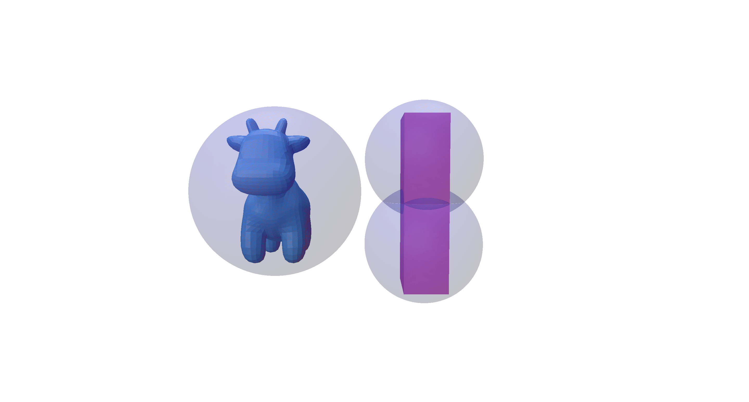
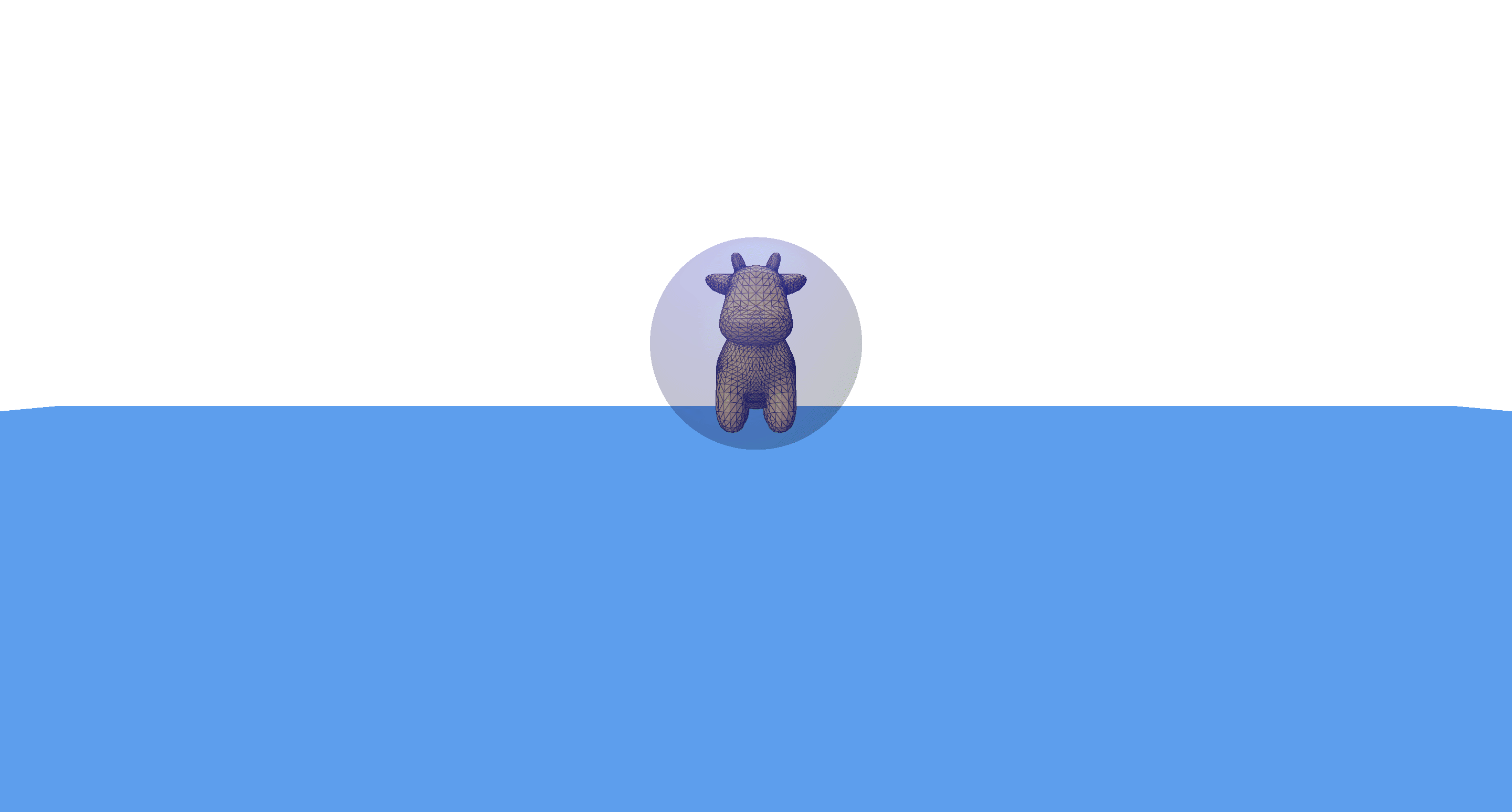
Figure 1: Our example 3D implementations of Gpytoolbox sweeping of Stanford bunny and Spot cow object across zig-zag trajectory
By Juan Parra, Kimberly Herrera, and Eleanor Wiesler
Project mentors: Silvia Sellán, Noam Aigerman
Introduction
Given a surface we can represent it moving along certain trajectory in space by a swept area or swept volume. It’s a good idea to take this approach to model 3D shapes or to detect a collision of the shape with another shape in its environment. There are several algorithms in the literature that address the construction of the surface of a swept volume in space, each taking their respective assumptions on the surface and the trajectory.
In our project we trained neural networks to predict the sweeping of a surface, and attempted to find the best representation of a neural network that deals with discontinuities that appear in the process.
Using Signed-Distance Functions to Model Shape Sweeping
By a swept volume we mean the trajectory that a solid moving through space made. The importance of representing a swept volume can go from art modeling to collision detection in robotics. We can model the swept volume of the solid motion as a surface in 3D. The goal of this project is to train neural networks to learn swept volumes, and so we conducted the experiments of this study using 2D shapes swept across a trajectory in the coordinate plane and evaluated resulting swept area. To study the trajectory or “sweeping” of these shapes, we used Signed Distance Functions (SDFs).
A signed distance function is a way to represent a closed orientable surface S in 3D (or a closed curve in 2D). This signed distance function (SDF) is given by a function:
\( D:\mathbb{R}^3\to\mathbb{R} \) such that \( |D(p)| = \min\{d(p,q)^2: q\in S\} \), and the sign of \( D(p) \) is negative if \( p \) is inside the surface and positive otherwise. The zero level set \( D^{-1}(0) \) is equal to the surface \( S \).
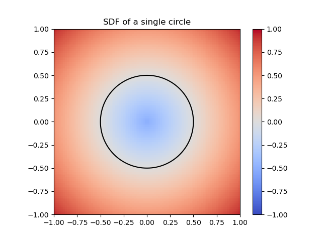
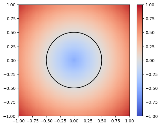
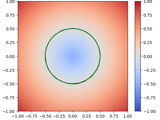
Given a signed distance function, we can use the Marching Cubes algorithm to construct a mesh representation of the surface. For example, \( G(x,y)=x^2 + y^2 -1 \) is the SDF of the unit circle.
Figure 1: SDF of a single circle
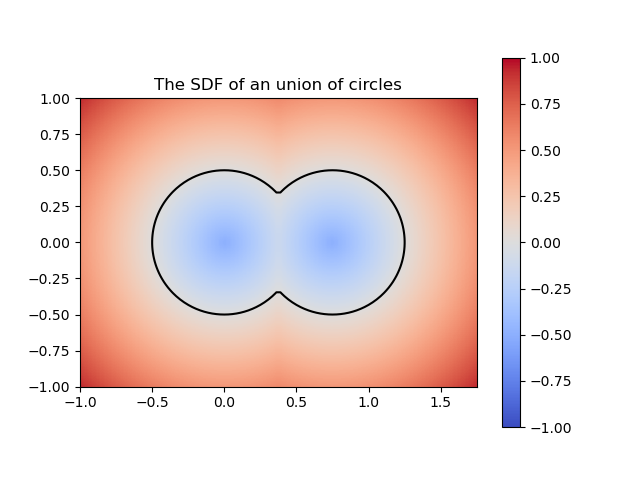
How to represent the SDF of the swept volume of a solid moving through space? We can leverage the operations between SDF’s to construct more complicated surfaces. For instance, the SDF of a unit circle is given by the function \( G(x,y) = x^2 + y^2 – 1 \) and the SDF of a translated circle to the right is \( H(x,y) = (x-0.75)^2 + y^2 – 1 \).
So if we wanted to paste both circles as if they were bubbles, we could define the union SDF as:
\[
\mathrm{union}(x,y)
=
\min\{
G(x,y), H(x,y)
\}
\]
Figure 2: SDF of a union of circles
If we want to perform a continuous motion of the solid we have to model it with a continuous function \(T: [0,1] \to SO(3)\) parametrized by the time, where
\(SO(3)\) is the set of rigid motions in 3D (abuse of notation to consider translations as well). Analogously we can think of rigid motions in 2D.
Suppose that \(F:\mathbb{R}^3 \to \mathbb{R}\) is the SDF of the solid we’re moving through space with the motion
\(T:[0,1] \to SO(3)\).
Then the swept volume of the solid is given by the SDF
$$
\text{swept volume}(\mathbf{x})
=
\min_{t\in[0,1]}
F(T_t^{-1}(\mathbf{x})).
$$
For the construction of a swept volume (or area) we can start with a previous
step, which is to define the function \(t^*:\mathbb{R}^3 \to \mathbb{R}\)
$$
t^*(\mathbf{x})
=
\mathrm{argmin}_{t\in [0,1]}
F(T_t^{-1}(\mathbf{x})),
$$
for which we will also have
$$
\text{swept volume}(\mathbf{x})
=
F
\left(
T_{t^*(\mathbf{x})}^{-1}
(\mathbf{x})
\right).
$$
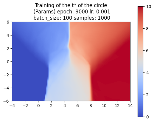
The \(t^*\) function now it’s a “piecewise” continuous function on its domain
as shown in the following figures.
Finite Stamping
In order to compute an approximation for the swept volume, one first approach will be to make finite stamping of the SDF moving along a finite discretized sequence of times
\(0= t_1< \cdots< t_n=1\) and then compute the SDF
$$
\text{swept volume approximation}(\mathbf{x})
=
\min_{t\in \{t_1, \ldots, t_n\}}
F(T_t^{-1}(\mathbf{x})).
$$
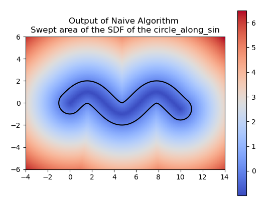
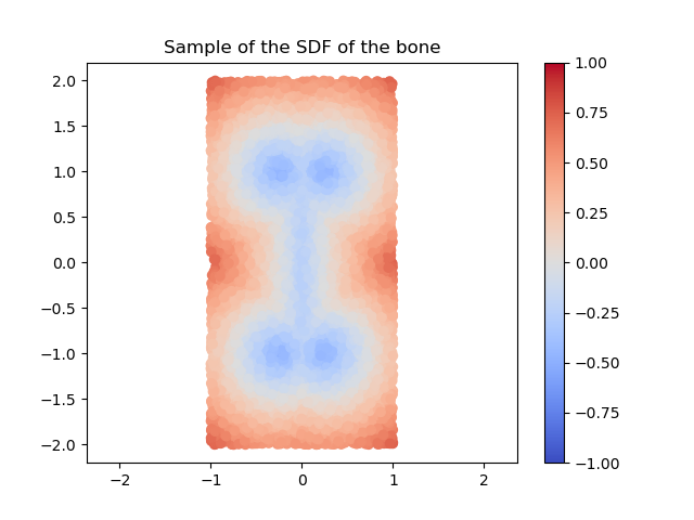
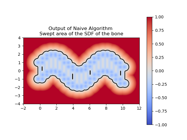
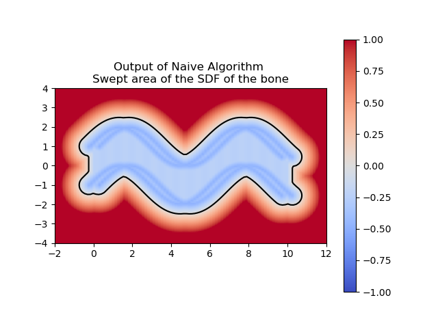
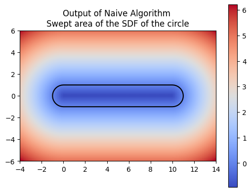
For example, if we define an SDF of a bone (see next 3 images),
and let's say we defined the motion \(T_t(x,y) = (x,y) + (t, \sin(t))\), then depending on how fine is our discretization, we can have a good or a bad approximation.
(a) 20 times
(b) 100 times
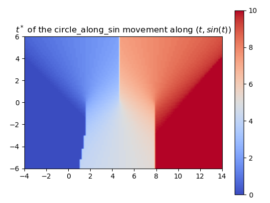
In this case we can also define an approximation to the \(t^*\) function as
follows
$$
t^*_{\text{approx}}(\textbf{x})
=
\text{argmin}_{t \in \{ t_1, \ldots, t_n \}}
F(T_{t}^{-1} (\mathbf{x})).
$$
However, we can notice that looking for the argument of the minimum
of a function can be computationally expensive, and that’s something we may want to do only once in our lifes.
Maybe we could substitute our Finite Stamping SDF with a neural network.
Knowing that \(t^*\) is not a continuous function, it will be interesting to fit a neural network to it, and play with its architecture so we find a neural network that represents better those discontinuities.
Learning Swept SDFs with Neural Networks
How to use a NN for SDFs
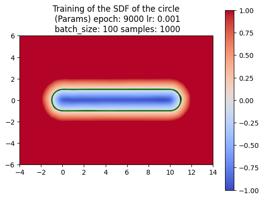
A neural network is just a function with many parameters; we can tweak these parameters to best approximate an SDF. To train the network, we first sample random points from the circle and compute their actual SDF values. The network’s goal is to predict these SDF values. By comparing the predicted values to the actual values using a loss function, the network can adjust its parameters to reduce the error. This adjustment is typically done through gradient descent, which iteratively refines the network’s parameters to minimize the loss. After training, we visualize the results to assess how well the neural network has learned to approximate the SDF. In the image below, the green represents the prediction for the circle by the neural network.
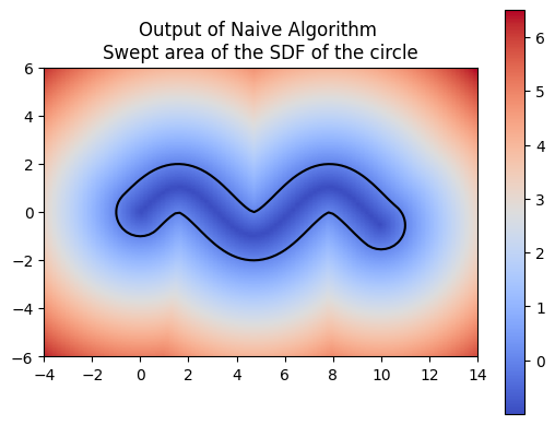
For computing a swept area, the neural network needs to approximate the union of multiple SDFs that together represent the swept area. Computing the swept area involves shifting the SDF along the trajectory at various points in time and then taking the union of all these SDFs. Once we understood how to compute the swept area ourselves, we had the neural network attempt the same. The following images show the results of our manual computation, which we refer to as the naive algorithm, for the sweeping of the circle along a horizontal path in comparison to the computation produced by the neural network. Similarly, the green represents the prediction for the swept area by the neural network.
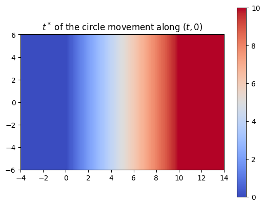
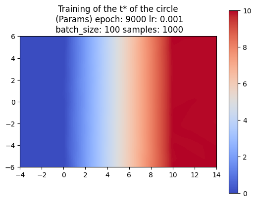
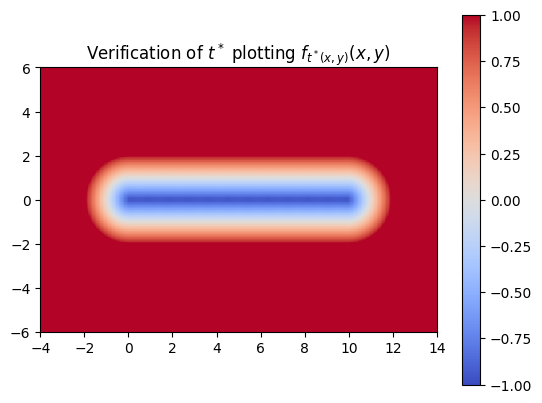
So far, we’ve trained the neural network to compute the SDF values for each point in a 2D grid. Now, since we are sweeping a shape over time, we want the network to return the times corresponding to these SDF values. We call these times t*. With the same shape and trajectory as above, the network has little issue doing this.
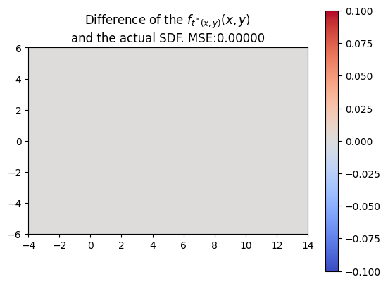
We also made sure that the t*‘s that we computed were producing the correct SDF of the swept area.
NN Difficulties detecting discontinuities
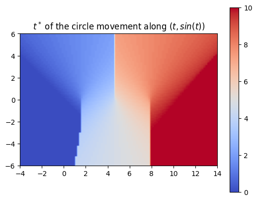
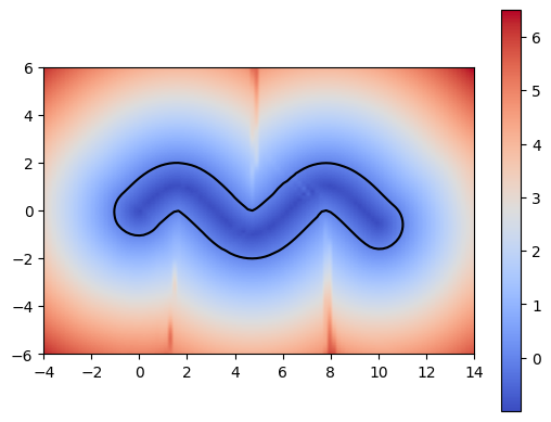
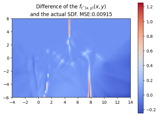
Using a more complex trajectory, such as a sine wave, introduces some challenges. While the neural network performs well in predicting the t* values, issues arise when computing the SDF with respect to these times. Specifically, the resulting SDF shows three lines emerging from the peaks and troughs of the curve. We can see this even more through the MSE plot.
The left image shows the sweeping of the circle using the t* values computed by the neural network.
These challenges become even more apparent when using shapes with sharper
edges such as a square. Because of this, we decided to work on optimizing the
neural network architecture.
Adjusting Our Neural Network Architecture
Changing Our Activation Function
Every neural network has a defined activation function. In the case of our preliminary neural network experiments above, the specified activation function was a Rectified Linear Unit (ReLU). Despite this, we did not achieve the most desirable outcome of minimal error in the predicted swept SDF versus the naive algorithm swept SDF. Specifically, we observed errors at sites of discontinuity, where there were changes in sign, for example.
In an attempt to improve neural network performance, we decided to experiment with different activation functions by altering our neural network architecture. Below, we present their corresponding results when used for swept SDF prediction.
Students: Eleanor Wiesler, Sara Samy, Juan Serratos
Collision detection is an important problem in interactive computer graphics and physics-based simulation that seeks to determine if, when and where two or more objects come into contact. [4] In this project, we implement bounded deformation trees (BD-Trees) and adapt this method to represent complex deformations of any geometry as linear superpositions of displacement fields.
Mesh deformationsusing modal analysis
When an object collides with a surface, we should expect the object to deform in some way, e.g. if a bouncing ball is thrown against a wall or dropped from a building, it should momentarily be “squished” or flattened at the site of collision. This is the effect we aim to accomplish using modal analysis.
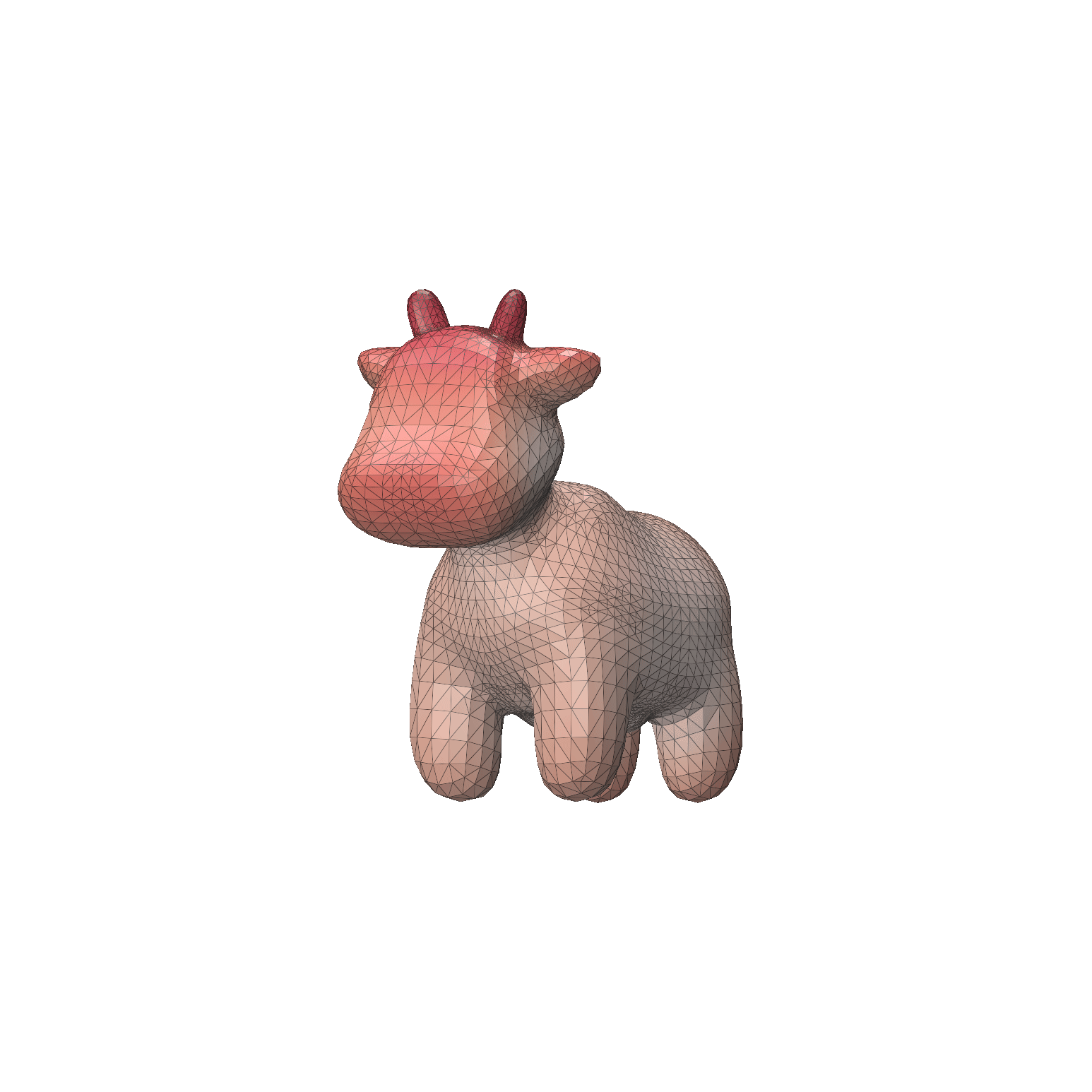
We start with a manifold triangular mesh e.g. Spot the cow, and tetrahedralize it using the python library of TetGen, a Delaunay-based tetrahedral mesh generator. [1] The resulting mesh is given as a \((V, C)\), where \(C\) is a set of tetrahedral cells whose vertices are in \(V\), as shown in Figure 1 below.
Figure 1: Tetrahedral mesh of Spot.
We use the Physics Based Animation Toolkit (PBAT) to compute the free vibrational modes of our model. Physically, one can describe vibration as the oscillatory motion of a physical structure, induced by energy exchanges of the potential (elastic deformation) and the kinetic (moving mass) energies. Vibrations are typically classified as either free or forced. In free vibrations, there are no continuous external forces acting on the structure, e.g. when a guitar string is plucked, while forced vibrations result from ongoing external forces. By looking at these free vibrations, we can determine the natural frequencies and normal modes of the structure.
First, we convert our geometricmesh into a FEM mesh and compute its Jacobian determinants and gradients of its shape function. You can check the documentation to learn more about FEM meshes.
Using these FEM quantities, we can model a hyperelastic material given its Young’s modulus \(Y\), Poisson’s ratio \(\nu\) and mass density \(\rho\).
rho = 1000.
Y = np.full(mesh.E.shape[1], 1e6)
nu = np.full(mesh.E.shape[1], 0.45)

# Compute mass matrix
M = pbat.fem.MassMatrix(mesh, detJeM, rho=rho, dims=3, quadrature_order=2).to_matrix()

# Define hyperelastic potential
hep = pbat.fem.HyperElasticPotential(mesh, detJeU, GNeU, Y, nu, energy=pbat.fem.HyperElasticEnergy.StableNeoHookean, quadrature_order=1)
Now we compute the Hessian matrix of the hyperelastic potential, and solve the generalized eigenvalue problem \(Av = \lambda M v\) using SciPy, where \(A\) denotes the Hessian matrix (a real symmetric matrix) and \(M\) denotes the mass matrix.
import scipy as sp

# Reshape matrix of vertices into a one-dimensional array
vs = mesh.X.reshape(mesh.X.shape[0]*mesh.X.shape[1], order="f")

hep.precompute_hessian_sparsity()
hep.compute_element_elasticity(vs)

HU = hep.hessian()
leigs, Veigs = sp.sparse.linalg.eigsh(HU, k=30, M=M, sigma=-1e-5, which="LM")
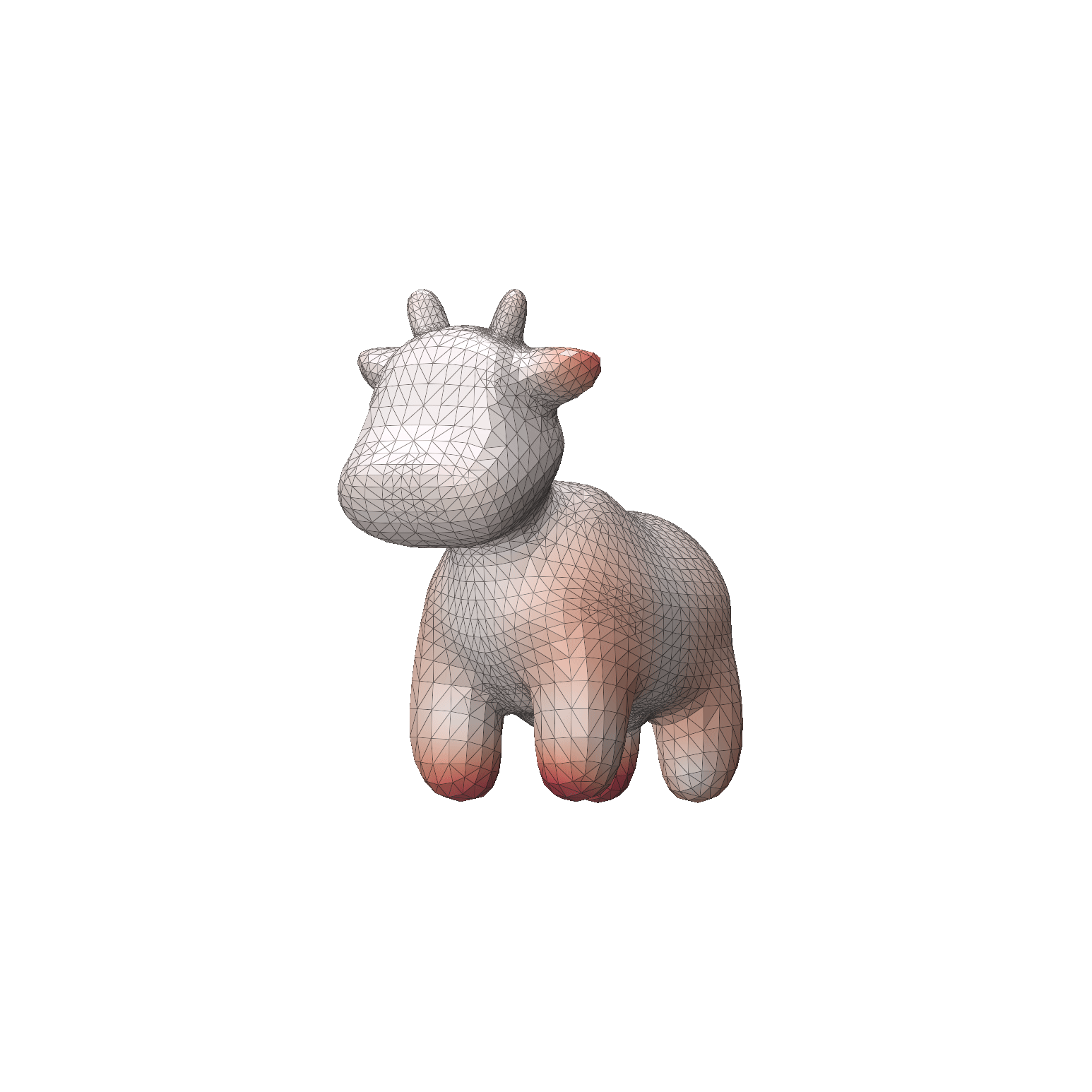
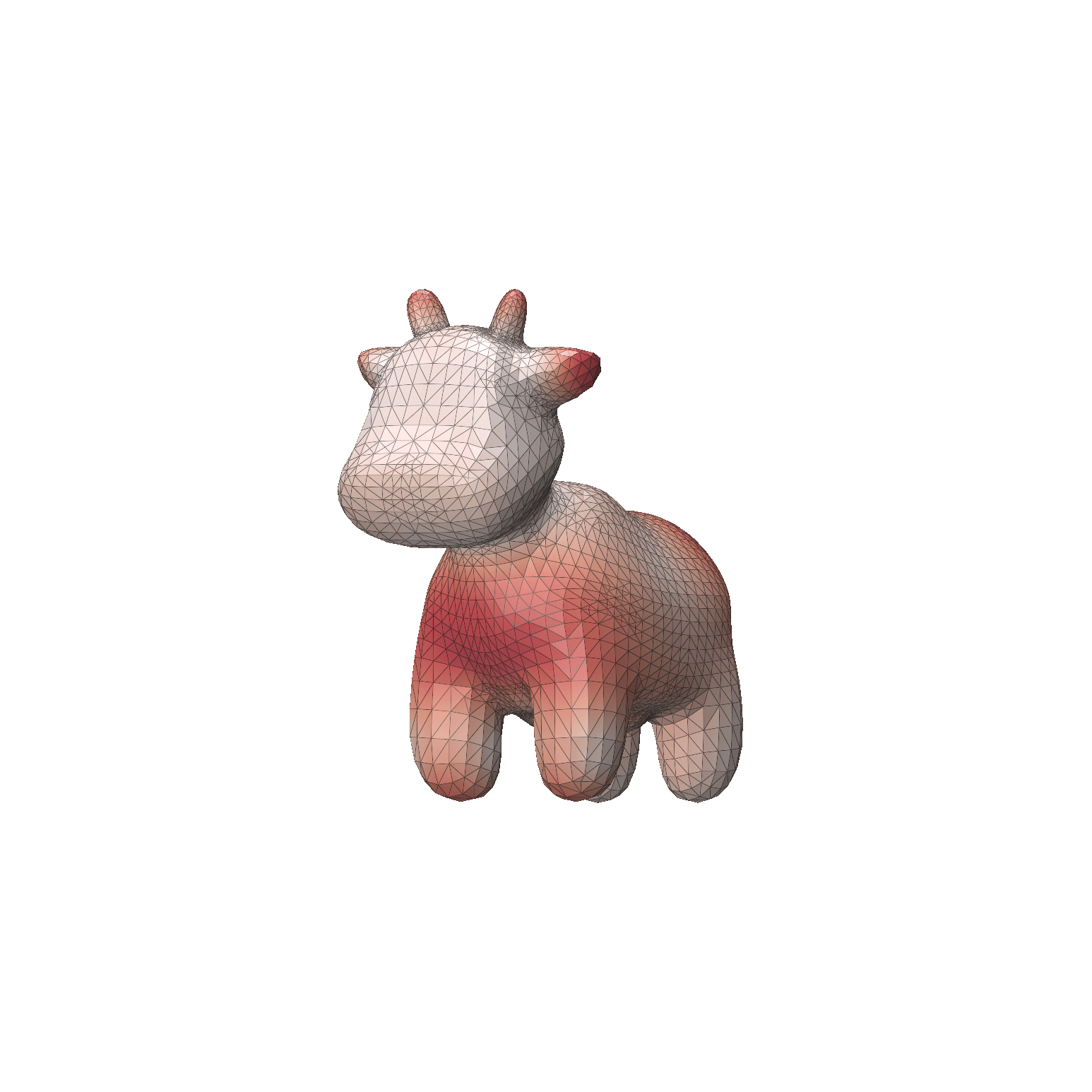
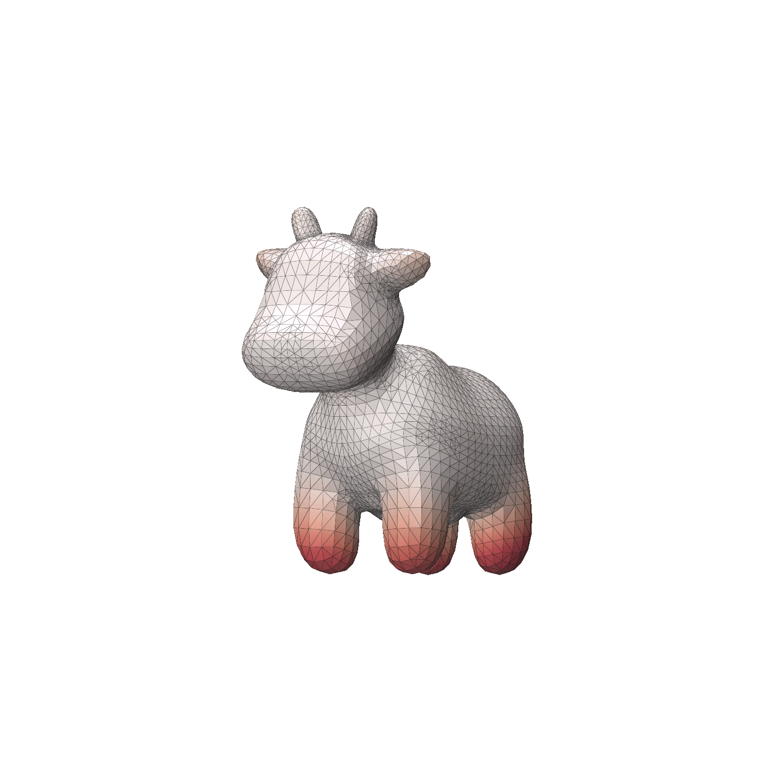
The resulting eigenvectors represent different deformation modes of the mesh. They can be animated as time continuous signals, as shown in Figure 2 below.
Figure 2: Six different deformation modes of Spot. Notice how each mode is characterized by deformations in a different local site of the mesh like its legs or neck.
Reduced Deformation Models
The BD-Tree paper [2] introduced the bounded deformation tree, which can perform collision detection for reduced deformable models at similar costs to standard algorithms for rigid bodies. But what do we mean exactly by reduced deformable models? First, unlike rigid bodies, where collisions affect only the position or movement of the object, deformable bodies can dynamically change their shape when forces are applied. Naturally, collision detection is simpler for rigid bodies than for deformable ones. Second, instead of explicitly tracking every individual triangle in a mesh, reduced deformable models represent complex deformations efficiently by a smaller set of parameters. This is achieved by using a linear superposition of pre-computed displacement fields that capture the essential ways a model can deform.
Suppose we have a triangular mesh with \(|V| = n\). Let \(\boldsymbol{p} \in \mathbb{R}^{3n}\) denote the undeformed vertices locations, and let \(U \in \mathbb{R}^{3n \times r}\) be a matrix with \(r \ll n\). Then the new deformed vertices location \(\boldsymbol{p’}\) are approximated by a linear superposition of \(r\) displacement fields given by the columns of \(U\) such that
where the amplitude of each displacement field is determined by the reduced coordinates \(\boldsymbol{q} \in \mathbb{R}^{r}\). Both \(U\) and \(\boldsymbol{q}\) must already be known in advance. In our case, the columns of \(U\) are the eigenvectors obtained from modal analysis described earlier, although they could also result from methods, e.g. an interpolation process. The reduced coordinates \(\boldsymbol{q}\) could also be determined by some possibly non-linear black box process. This is important to note: although the shape model is linear, the deformation process itself can be arbitrary!
Bounded deformation trees
Welzl’s algorithm
The BD-Tree works by constructing a hierarchy of minimum bounding spheres. As a first step, we need a method to construct the smallest enclosing sphere for some set of points. Fortunately, this problem has been well studied in the field of computational geometry, and we can use the randomized recursive algorithm of Welzl [3] that runs in expected linear time.
The Welzl’s algorithm is based on a simple observation: assume a minimum bounding sphere \(S\) has been computed a set of points \(P\). If a new point \(p\) is added to \(P\), then \(S\) needs to be recomputed only if \(p\) lies outside of \(S\), and the new point \(p\) must lie on the boundary of the new minimum bounding sphere for the points \(P \cup \{p\}\). So the algorithm keeps track of the set of input points and a set of support, which contains the points from the input set that must lie on the boundary of the minimum bounding sphere.
Sphere WelzlSphere(Point pt[], unsigned int numPts, Point sos[], unsigned int numSos)
{
	// if no input points, the recursion has bottomed out.
    // Now compute an exact sphere based on points in set of support (zero through four points)
	if (numPts == 0) {
		switch (numSos) {
			case 0: return Sphere();
			case 1: return Sphere(sos[0]);
			case 2: return Sphere(sos[0], sos[1]);
			case 3: return Sphere(sos[0], sos[1], sos[2]);
			case 4: return Sphere(sos[0], sos[1], sos[2], sos[3]);
		}
	}
	// Pick a point at "random" (here just the last point of the input set)
	int index = numPts - 1;
	// Recursively compute the smallest bounding sphere of the remaining points
	Sphere smallestSphere = WelzlSphere(pt, numPts - 1, sos, numSos);
	// If the selected point lies inside this sphere, it is indeed the smallest
	if(PointInsideSphere(pt[index], smallestSphere))
		return smallestSphere;
	// Otherwise, update set of support to additionally contain the new point
	sos[numSos] = pt[index];
	// Recursively compute the smallest sphere of remaining points with new s.o.s.
	return WelzlSphere(pt, numPts - 1, sos, numSos + 1);
}
The BD-Tree Method
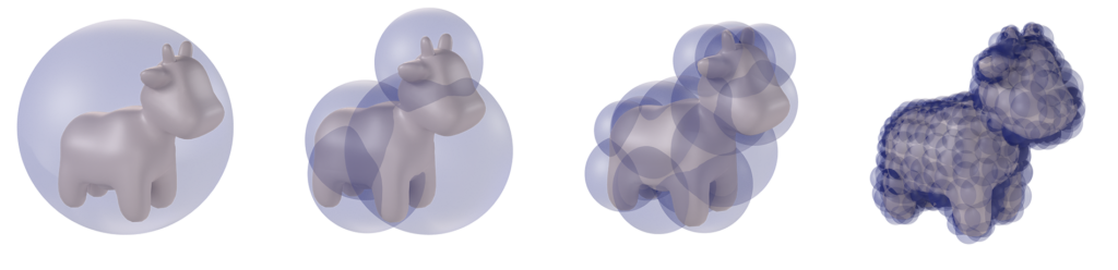
Figure 3: Wrapped BD-Tree for Spot at increasing recursion levels.
Now that we can compute the minimum bounding spheres for any set of points, we are ready to construct a hierarchical sphere tree on the undeformed model, after which it can be updated following deformation. First we note that the BD-Tree is a wrapped hierarchy, wherein the bounding spheres tightly enclose the underlying geometry but any bounding sphere at one level need not contain its child spheres. This is different from a layered hierarchy in which spheres must enclose their child spheres, but can fit the underlying geometry more loosely (see Figure 4).
Figure 4: An illustration—re-created from [2] of the wrapped hierarchy (left) and layered hierarchy (right). The underlying geometry is shown in green with five vertices and four edges.
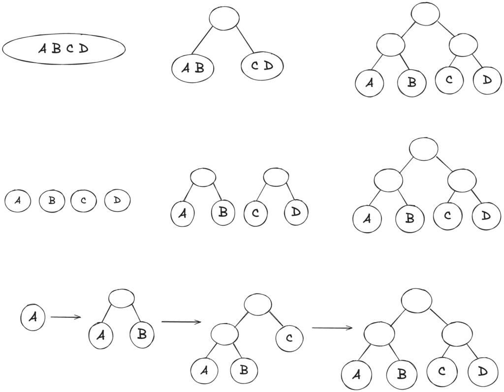
As shown in Figure 5, there are many possible approaches to building a binary tree. In our case, we use a simple top-down approach while partitioning the underlying geometry, i.e. we recursively split Spot at its median into two parts with respect to its local coordination axes, such that a leaf node (the lowest level) contains only one triangle.
Figure 5: Hierarchical binary tree construction with four objects using a top-down (top), bottom-up (middle) and insertion approach (bottom).
As the object deforms, how do we compute the new bounding spheres quickly and efficiently?
Let \(S\) denote a sphere in the hierarchical tree with center \(c\) and radius \(R\) containing the \(k\) points of the geometry \(\{p_{i}\}_{1 \leq i \leq k}\). After the deformation, the center of the sphere \(c\) is displaced by a weighted average of the contained points’ displacements \(u_{i}\) with weights \(\beta_i\) e.g. \(\beta_i := 1/k\) for \(1 \leq i \leq k\). So the new center can be expressed as
\(\displaystyle c’ = c + \sum_{i = 1}^{k} \beta_i u_i.\)
Using the displacement equation above, we can write \(u_i\) as the sum \(\sum_{j = 1}^{r} U_{ij} q_{j}\) and substitute this into the previous equation to obtain:
\(\displaystyle c’ = c + \sum_{j = 1}^{r} \left(\sum_{i = 1}^{k} \beta_i U_{ij}\right) q_j = c + \bar{U} \boldsymbol{q}.\)
To compute the new radius \(R’\), we make use of the triangle inequality
Thus, we have an updated bounding sphere \(S’\) with its center \(c’\) and radius \(R’\) computed as functions of the reduced coordinates \(\boldsymbol{q}\).
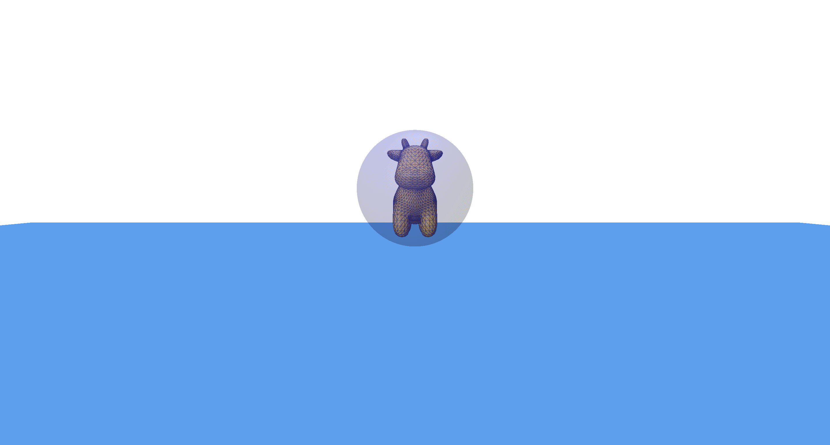
Figure 6: Spot colliding with ground plane. The colors of the spheres change based on the ratio of \(R\) in the undeformed state to \(R’\) in the deformed state.
References
[1] Hang Si. TetGen, a Delaunay-based quality tetrahedral mesh generator. ACM Transactions on Mathematical Software, 41(2), 2015.
[2] Doug L. James and Dinesh K. Pai. BD-Tree: Output-Sensitive Collision Detection for Reduced Deformable Models. ACM Transactions on Graphics, 23(3), 2004.
[3] Emo Welzl. Smallest enclosing disks (balls and ellipsoids). New Results and New Trends in Computer Science, 555, 1991.
[4] Christer Ericson. Real-Time Collision Detection. CRC Press, Taylor & Francis Group. Chapter 4, p. 99-100. 2005.
Primary mentors: Silvia Sellán, University of Toronto and Oded Stein, University of Southern California
Volunteer assistant: Andrew Rodriguez
Fellows: Johan Azambou, Megan Grosse, Eleanor Wiesler, Anthony Hong, Artur RB Boyago, Sara Samy
After talking about what are some of the ways to reconstruct sdfs (see part one), we now study the question of how to evaluate their performance. Two classes of error function are considered, the first more inherent to our sdf context, and the second more general in all situations. We will first show results by our old friends, Chamfer distance, Hausdorff distance, and area method (see here for example), and then introduce the inherent one.
Hausdorff and Chamfer Distance
The Chamfer distance provides an average-case measure of the dissimilarity between two shapes. It calculates the sum of the distances from each point in one set to the nearest point in the other set. This measure is particularly useful when the goal is to capture the overall discrepancy between two shapes while being less sensitive to outliers. The Chamfer distance is defined as: $$ d_{\mathrm{Chamfer }}(X, Y):=\sum_{x \in X} d(x, Y)=\sum_{x \in X} \inf _{y \in Y} d(x, y) $$
The Bi-Chamfer distance is an extension that considers the average of the Chamfer distance computed in both directions (from \(X\) to \(Y\) and from \(Y\) to \(X\) ). This bidirectional measure provides a more balanced assessment of the dissimilarity between the shapes: $$ d_{\mathrm{B} \mathrm{-Chamfer }}(X, Y):=\frac{1}{2}\left(\sum_{x \in X} \inf {y \in Y} d(x, y)+\sum{y \in Y} \inf _{x \in X} d(x, y)\right) $$
The Hausdorff distance, on the other hand, measures the worst-case scenario between two shapes. It is defined as the maximum distance from a point in one set to the closest point in the other set. This distance is particularly stringent because it reflects the largest deviation between the shapes, making it highly sensitive to outliers.
The formula for Hausdorff distance is: $$ d_{\mathrm{H}}^Z(X, Y):=\max \left(\sup {x \in X} d_Z(x, Y), \sup {y \in Y} d_Z(y, X)\right) $$
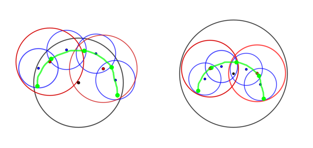
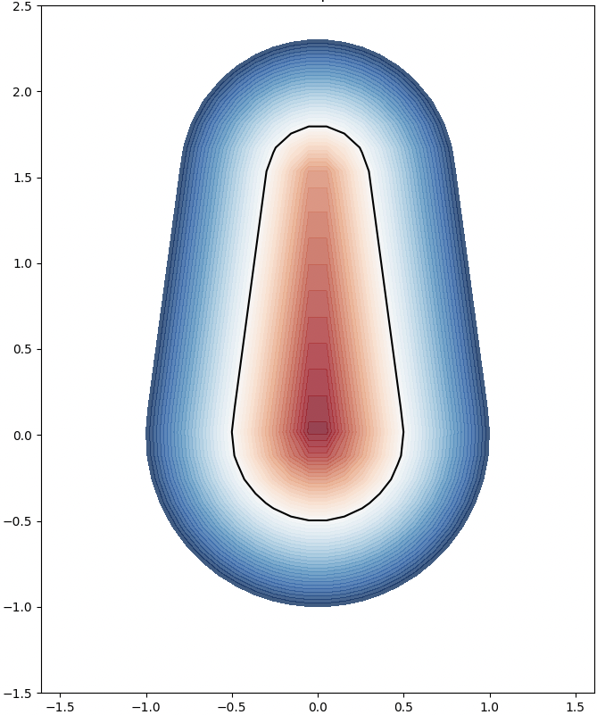
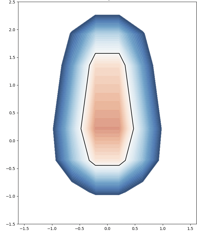
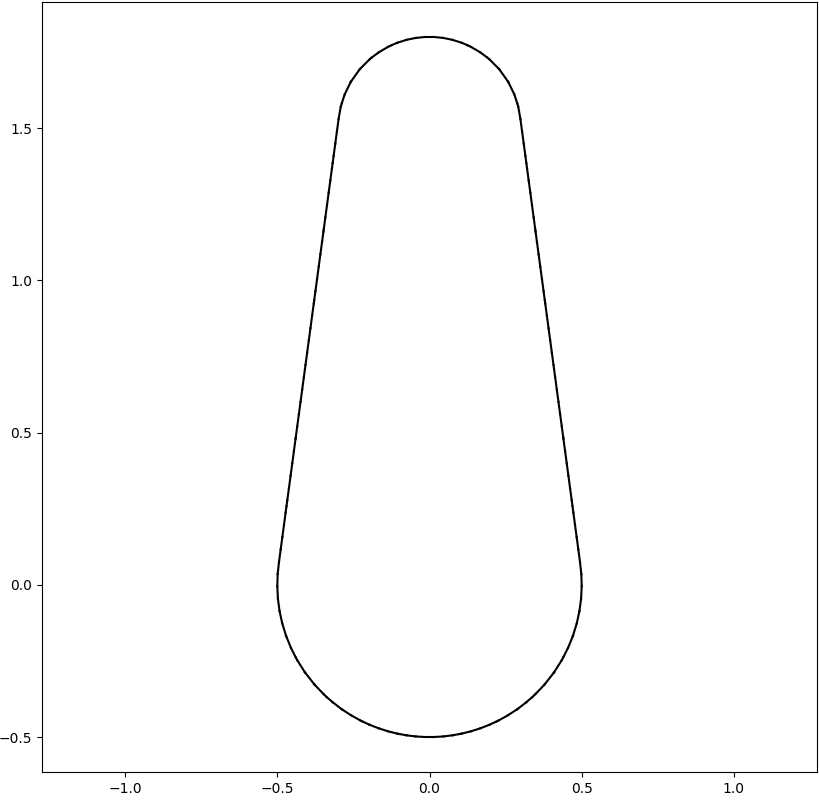
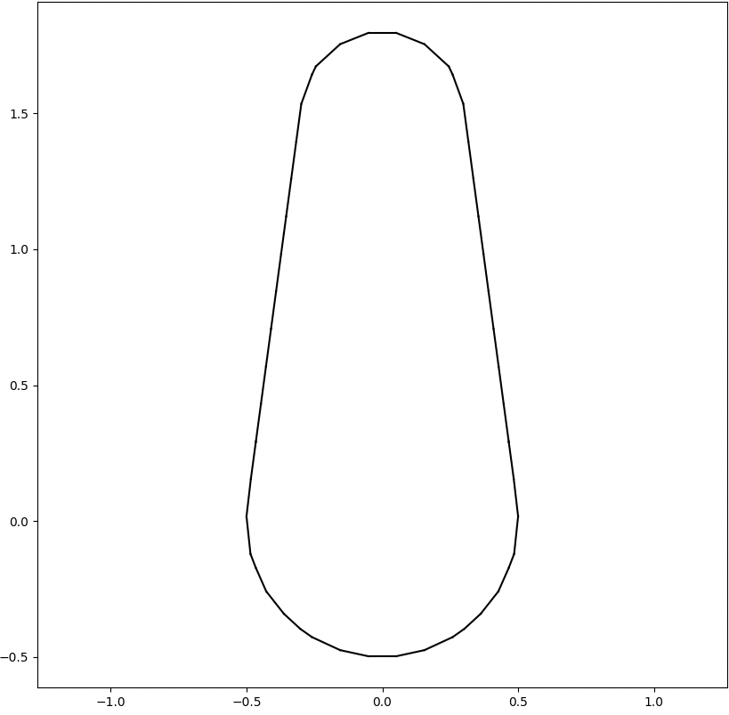
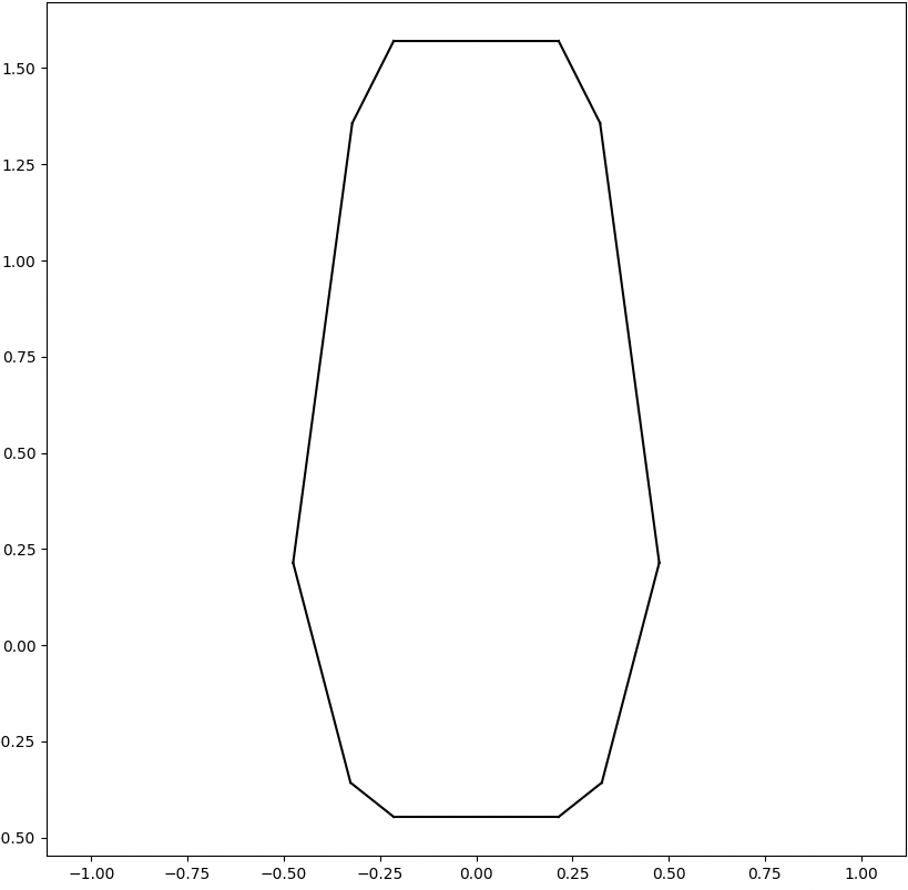
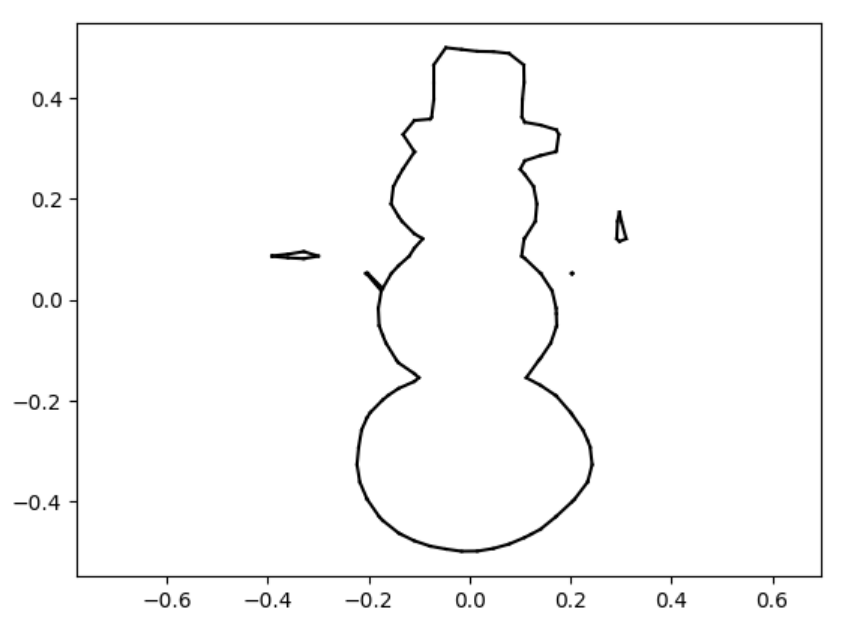
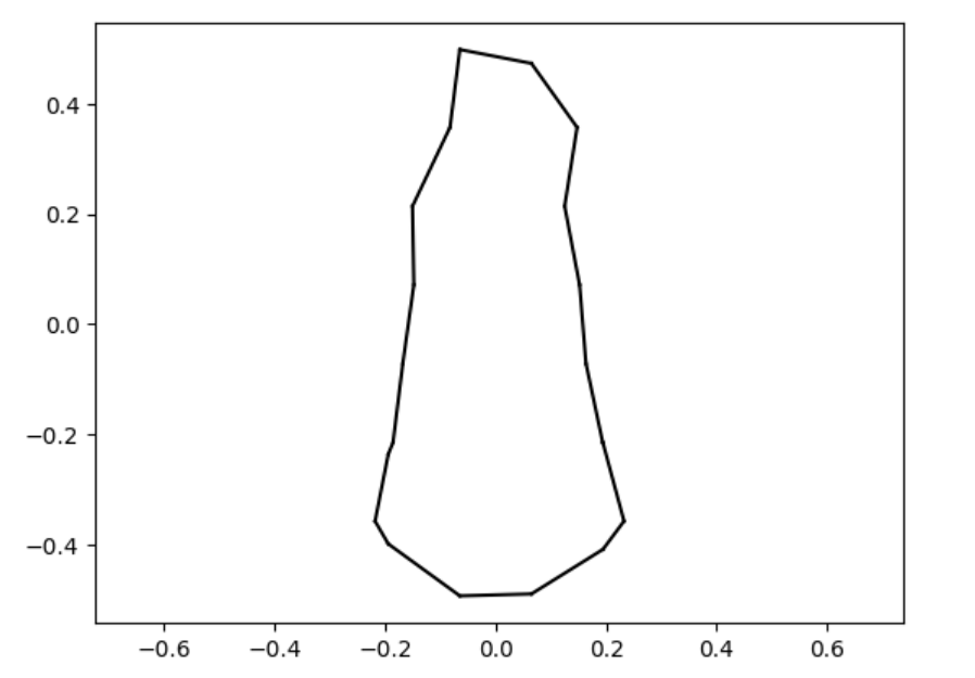
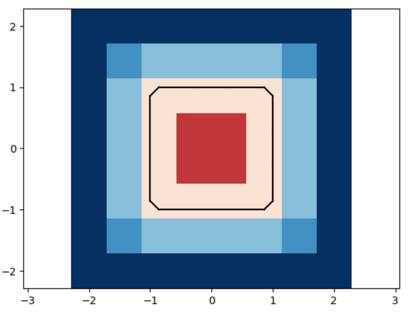
We analyze the Hausdorff distance for the uneven capsule (the shape on the right; exact sdf taken from there) in particular.
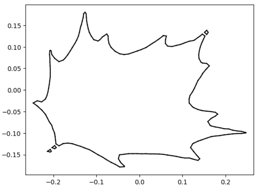
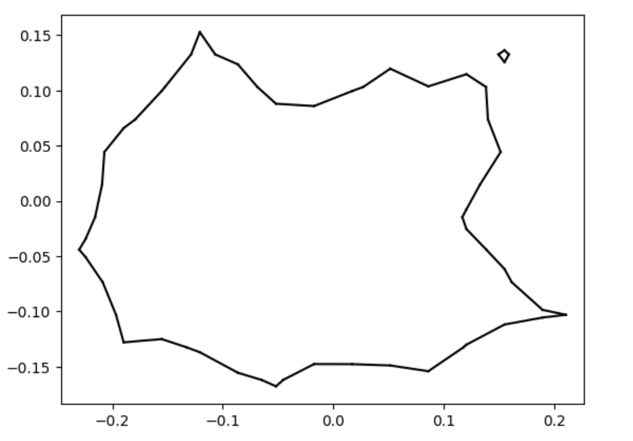
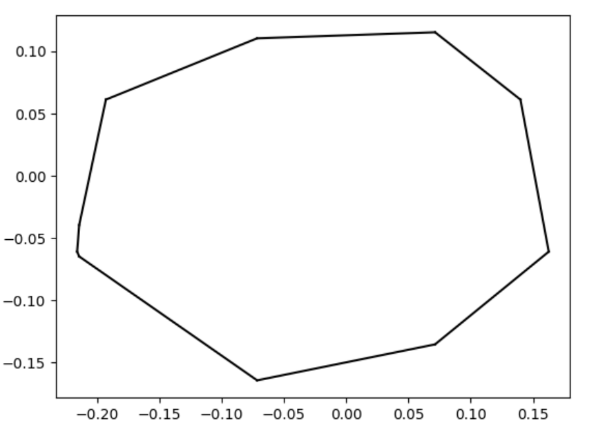
This plot visually compares the original zero level set (ground truth) with the reconstructed polyline generated by the marching squares algorithm at a specific resolution. The black dots represent the vertices of the polyline, showing how closely the reconstruction matches the ground truth, demonstrating the efficacy of the algorithm at capturing the shape’s essential features.
This plot shows the relationship between the Hausdorff distance and the resolution of the reconstruction. As resolution increases, the Hausdorff distance decreases, illustrating that higher resolutions produce more accurate reconstructions. The log-log plot with a linear fit suggests a strong inverse relationship, with the slope indicating a nearly quadratic decrease in Hausdorff distance as resolution improves.
Area Method for Error
Another error method we explored in this project is an area-based method. To start this process, we can overlay the original polyline and the generated polyline. Then, we can determine the area between the two, counting all regions as positive area. Essentially, this means that if we take values inside a polyline to be negative and outside a polyline to be positive, the area counted as error consists of the set of all regions where the sign of the original polyline’s SDF is not equal to the sign of the generated polyline’s SDF. The resultant area corresponds to the error of the reconstruction.
Here is a simple example of this area method using two quadrilaterals. The area between them is represented by their union (all blue area) with their intersection (the darker blue triangle) removed:
Here is an example of the area method applied to a star, with the area quantity corresponding to error printed at the top:
Inherent Error Function
We define the error function between the reconstructed polyline and the zero level set (ZLS) of a given signed distance function (SDF) as: $$ \mathrm{Error}=\frac{1}{|S|} \sum_{s \in S} \mathrm{sdf}(s) $$
Here, \(S\) represents a set of sample points from the reconstructed polyline generated by the marching squares algorithm, and \(|\mathrm{S}|\) denotes the cardinality of this set. The sample points include not only the vertices but also the edges of the reconstructed polyline.
The key advantage of this error function lies in its simplicity and directness. Since the SDF inherently encodes the distance between any query point and the original polyline, there’s no need to compute distances separately as required in Hausdorff or Chamfer distance calculations. This makes the error function both efficient and well-suited to our specific context, providing a more streamlined and integrated approach to measuring the accuracy of the reconstruction.
Note that one variant one can consider is to square the \(\mathrm{sdf}(s)\) part to get rid of the signed nature, because the signs can cancel with each other for the reconstructed polyline is not always entirely inside the ground truth or entirely cotains the ground truth.
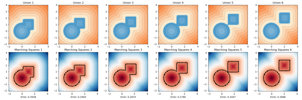
Below are one experiment we did for computing using this inherent error function, the unsquared one. We let the circle sdf be fixed and let the square sdf “escape” from the circle in a constant speed of \(0.2\). That is, we used the union of a fixed circle and a square with changing position as a series of shapes to do analysis. We then draw with color map used in this repo for the ground truths and the marching square results using the common color map.
The inherent error of each union After several trials, one simple observation drawn from this escapaing motion is that when two shapes are more confounding with each other, as in the initial stage, the error is higher; and when the image starts to have two separated connected components, the error rises again. The first one can perhaps be explained by what the paper pointed out as pseudo-sdfs, and the second one is perhaps due to occurence of multipal components.
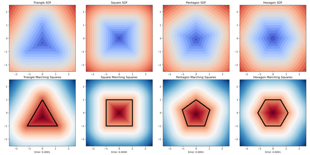
Here is another experiment. We want to know how well this method can simulate the physical characteristics of an object’s rugged level. We used a series of regular polygons. Although the result is theoretically unintheresting as the errors are all nearly zero, this is visually conformting.
Primary mentors: Silvia Sellán, University of Toronto and Oded Stein, University of Southern California
Volunteer assistant: Andrew Rodriguez
Fellows: Johan Azambou, Megan Grosse, Eleanor Wiesler, Anthony Hong, Artur, Sara
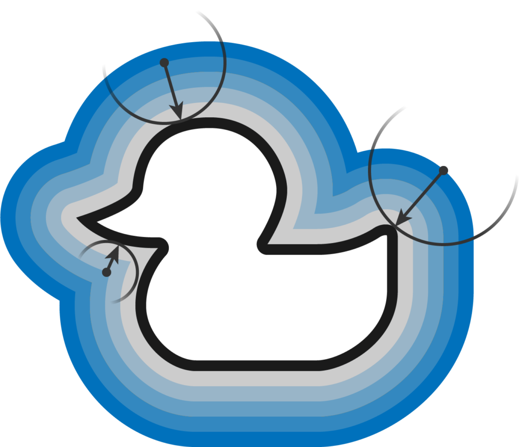
The definition of SDFs using ducks
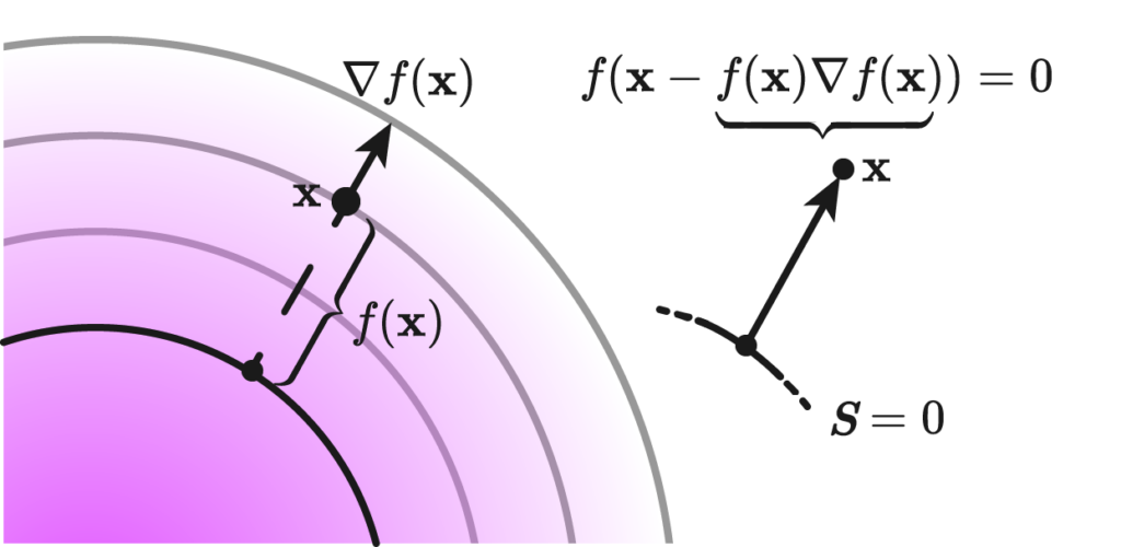
Suppose that you took a piece of metal wire, twisted into some shape you like, let’s make it a flat duck, and then put it on a little pond. The splash of water made by said wire would propagate as a wave all across the pond, inside and outside the wire. If the speed of the wave were \(1 m/s \), you’d have, at every instant, a wavefront telling you exactly how far away a given point is from the wire.
This is the principle behind a distance field, a scalar valued field \( d(\mathbf{x}) \) whose value at any given point \(\mathbf{x}\) is given by\( d(\mathbf{x}, S) = \min_{\mathbf{y}}d(\mathbf{x}, \mathbf{y})\), where \( S \)is a simpled closed curve. To make this a signed distance field, we can distinguish between the interior and exterior of the shape by adding a minus sign in the interior region.
Suppose we were to define sdf without knowing the boundary \(S\); given a region \( \Omega \) and a surface \( S \), whose inside is defined as the closure of \( \overline{\Omega} = A \). A function \( f : \mathbb{R}^n \rightarrow \mathbb{R} \) is said to be a signed distance function if for every point \( \mathbf{x} \in \Omega \) , we have eikonality \( | \nabla f | = 1 \) and closest point condition: \[ f( \mathbf{x} – f(\mathbf{x}) \nabla f(\mathbf{x})) = 0 \]
The statement reads very simply: if we have a point \( \mathbf{x} \), and take the difference vector to the normal of the level set at hand times the distance, it should take us to the point \( \mathbf{x} \) closest to the zero level set.
This second definition is equivalent to the first one by an observation that eikonality implies \(1\)-Lipschitz property of the function \(f\) and it is also used for the last step of the following derivation: \(\exists q \in S:=f^{-1}(0)\) $$ p-f(p) \nabla f(p)=q \Longrightarrow p-q=f(p) \nabla f(p) \Longrightarrow|p-q|=|f(p)| $$
This combined with \(1\)-Lipschitz property gives a proof of contradiction for characterization of sdf by eikonality and closest point condition.
Our project was focused on the SDF-to-Surface reconstruction methods, which is, given a SDF, how can we make a surface out of it? I’ll first tell you about the much simpler problem, which is Surface-to-SDF.
Our SDFs
To lay the foundation, we started with the 2D case: SDFs in the plane from which we can extract polylines. Before performing any tests, we needed a database of SDFs to work with. We created our SDFs using two different skillsets: art and math.
The first of our SDFs were hand-drawn, using an algorithm that determined the closest perpendicular distance to a drawn image at the number of points in a grid specified by the resolution. This grid of distance values was then converted into a visual representation of these distance values – a two-dimensional SDF. Here are some of our hand-drawn SDFs!
The second of our SDFs were drawn using math! Known as exact SDFs, we determined these distances by splitting the plane into regions with inequalities and many AND/OR statements. Each of these regions was then assigned an individual distance function corresponding to the geometry of that space. Here are some of our exact SDF functions and their extracted polylines!
Exact vs. Drawn
Exact Signed Distance Functions (SDFs) provide precise, mathematically rigorous measurements of the shortest distance from any point to the nearest surface of a shape, derived analytically for simple forms and through more complex calculations for intricate geometries. These are ideal for applications demanding high precision but can be computationally intensive. Conversely, drawn or approximate SDFs are numerically estimated and stored in discretized formats such as grids or textures, offering faster computation at the cost of exact accuracy. These are typically used in digital graphics and real-time applications where speed is crucial and minor inaccuracies in distance measurements are acceptable. The choice between them depends on the specific requirements of precision versus performance in the application.
Operations on SDFs
For two SDFs, \(f_1(x)\) and \(f_2(x)\), representing two shapes, we can define the following operations from constructive geometry:
We used these operations to create the following new sdfs: a cat and a tessellation by hexagons.
Marching Squares Reconstructions with Multiple Resolutions
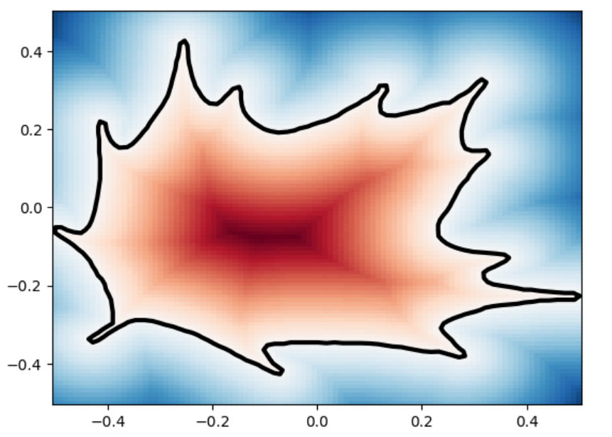
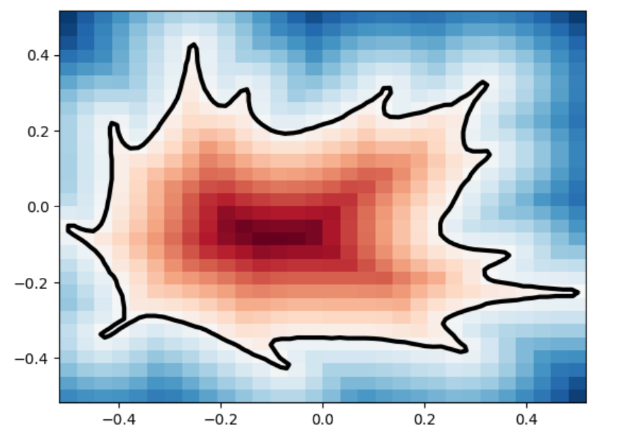
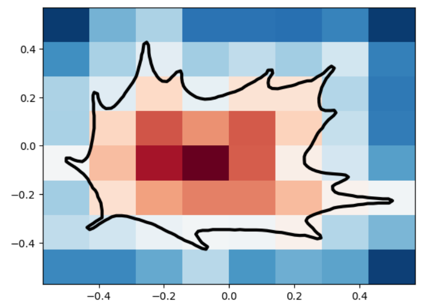
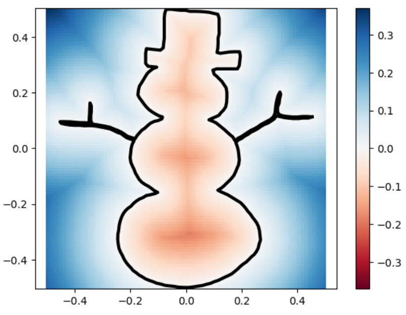
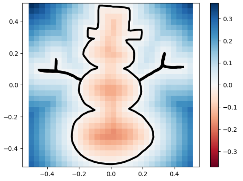
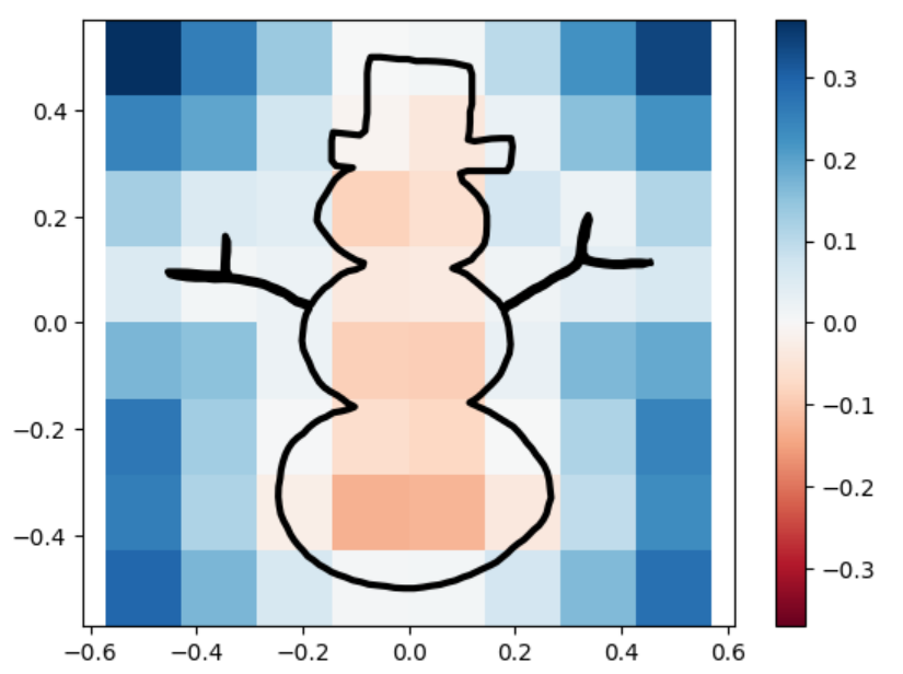
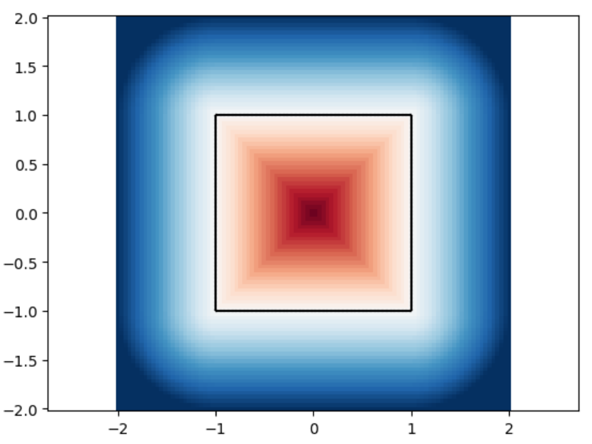
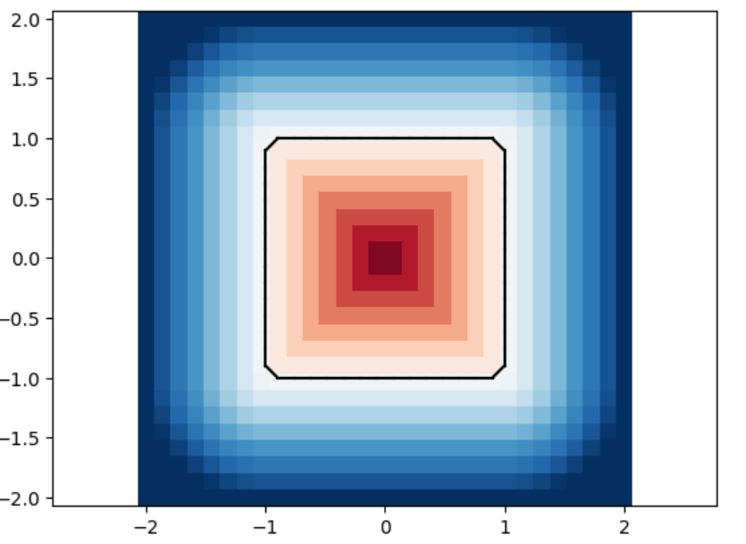
The marching_squares algorithm is a contouring method used to extract contour lines (isocontours) or curves from a two-dimensional scalar field (grid). It’s the 2D analogue of the 3D Marching Cubes algorithm, widely used for surface reconstruction in volumetric data. When applied to Signed Distance Functions (SDFs), marching_squares provides a way to visualize the zero level set (the exact boundary) of the function, which represents the shape defined by the SDF. Below are visualizations of various SDFs which we passed into marching squares with varied resolutions in order to test how well it reconstructs the original shape.
SDF / Resolution
100×100
30×30
8×8
leaf
leaf marching_squares
uneven capsule
uneven capsule marching_squares
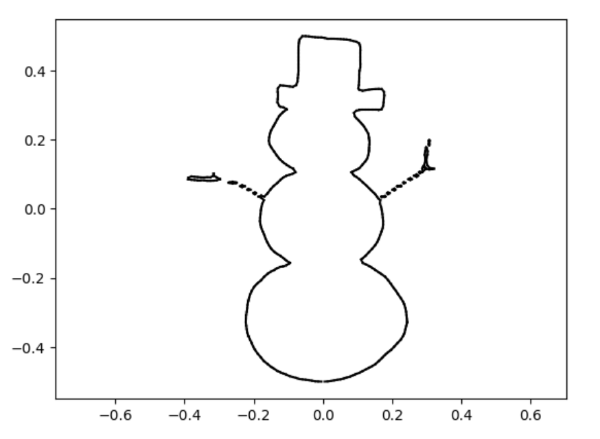
snowman
snowman marching_squares
square
square marching_squares
sdfs and reconstructions in three different resolutions.
SDFs in 3D Geometry Processing
While the work we have done has been 2D in our project, signed-distance functions can be applied to 3D geometry meshes in the same way. Below are various examples from recent papers that use signed distance functions in the 3D setting. Take for example marching cubes, a method for surface reconstruction in volumetric data developed by Lorensen and Cline in 1987 that was originally motivated by medical imaging. If we start with an implicit function, then the marching cubes algorithm works by “marching” over a uniform grid of cubes and then locating the surface of interest by seeing where the surface intersects with the cubes, and adding triangles with each iteration such that a triangle mesh can ultimately be formed via the union of each triangle. A helpful visualization of this algorithm can be found here.
Take for example our mentors Silvia Sellán and Oded Stein’s recent paper “Reach For the Spheres:Tangency-Aware Surface Reconstruction of SDFs” with C. Batty which introduces a new method for reconstructing an explicit triangle mesh surface corresponding to an SDF, an algorithm that uses tangency information to improve reconstructions, and they compare their improved 3D surface reconstructions to marching cubes and an algorithm called Neural Dual Contouring. We can see from their figure below that their SDF and tangency-aware and reconstruction algorithm is more accurate than marching cubes or NDCx.
(From Sellan et al, 2024) The Reach for the Spheres method that using tagency information for more accurate surface reconstructions can be seen on both 10^3 and 50^3 SDF grids as being more accurate than competing methods of marching cubes and NDCx. They used features of SDF and the idea of tangency constraints for this novel algorithm.
Another SGI mentor, Professor Keenan Crane, also works with signed distance functions. Below you can see in his recent paper “A Heat Method for Generalized Signed Distance” with Nicole Feng, they introduce a novel method for SDF approximation that completes a shape if the geometric structure of interest has a corrupted region like a hole.
(From Feng and Crane, 2024): In this figure, you can see that the inputted curves in magenta are broken, and the new method introduced by Feng and Crane works by computing signed distances from the broken curves, allowing them to ultimately generate an approximated SDF for the corrupted geometry where other methods fail to do this.
Clearly, SDFs are beautiful and extremely useful functions for both 2D and 3D geometry tasks. We hope this introduction to SDFs inspires you to study or apply these functions in your future geometry-related research.
References
Sellán, Silvia, Christopher Batty, and Oded Stein. “Reach For the Spheres: Tangency-aware surface reconstruction of SDFs.” SIGGRAPH Asia 2023 Conference Papers. 2023.
Feng, Nicole, and Keenan Crane. “A Heat Method for Generalized Signed Distance.” ACM Transactions on Graphics (TOG) 43.4 (2024): 1-19.
Marschner, Zoë, et al. “Constructive solid geometry on neural signed distance fields.” SIGGRAPH Asia 2023 Conference Papers. 2023.