Project mentor: Prof. Paul Kry
Students: Eleanor Wiesler, Sara Samy, Juan Serratos
Collision detection is an important problem in interactive computer graphics and physics-based simulation that seeks to determine if, when and where two or more objects come into contact. [4] In this project, we implement bounded deformation trees (BD-Trees) and adapt this method to represent complex deformations of any geometry as linear superpositions of displacement fields.
Mesh deformations using modal analysis
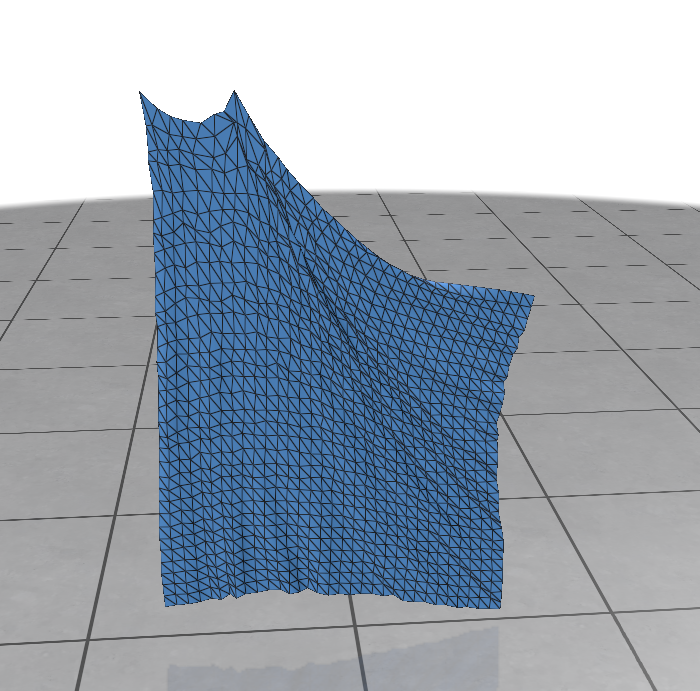
When an object collides with a surface, we should expect the object to deform in some way, e.g. if a bouncing ball is thrown against a wall or dropped from a building, it should momentarily be “squished” or flattened at the site of collision. This is the effect we aim to accomplish using modal analysis.
We start with a manifold triangular mesh e.g. Spot the cow, and tetrahedralize it using the python library of TetGen, a Delaunay-based tetrahedral mesh generator. [1] The resulting mesh is given as a \((V, C)\), where \(C\) is a set of tetrahedral cells whose vertices are in \(V\), as shown in Figure 1 below.
We use the Physics Based Animation Toolkit (PBAT) to compute the free vibrational modes of our model. Physically, one can describe vibration as the oscillatory motion of a physical structure, induced by energy exchanges of the potential (elastic deformation) and the kinetic (moving mass) energies. Vibrations are typically classified as either free or forced. In free vibrations, there are no continuous external forces acting on the structure, e.g. when a guitar string is plucked, while forced vibrations result from ongoing external forces. By looking at these free vibrations, we can determine the natural frequencies and normal modes of the structure.
First, we convert our geometric mesh into a FEM mesh and compute its Jacobian determinants and gradients of its shape function. You can check the documentation to learn more about FEM meshes.
import meshio
import numpy as np
import pbatoolkit as pbat

imesh = meshio.read("./spot.mesh")
V, C = imesh.points, imesh.cells_dict["tetra"]

mesh = pbat.fem.Mesh(V.T, C.T, element=pbat.fem.Element.Tetrahedron, order=1)

GNeU = pbat.fem.shape_function_gradients(mesh, quadrature_order=1)
detJeM = pbat.fem.jacobian_determinants(mesh, quadrature_order=2)
detJeU = pbat.fem.jacobian_determinants(mesh, quadrature_order=1)
Using these FEM quantities, we can model a hyperelastic material given its Young’s modulus \(Y\), Poisson’s ratio \(\nu\) and mass density \(\rho\).
rho = 1000.
Y = np.full(mesh.E.shape[1], 1e6)
nu = np.full(mesh.E.shape[1], 0.45)

# Compute mass matrix
M = pbat.fem.MassMatrix(mesh, detJeM, rho=rho, dims=3, quadrature_order=2).to_matrix()

# Define hyperelastic potential
hep = pbat.fem.HyperElasticPotential(mesh, detJeU, GNeU, Y, nu, energy=pbat.fem.HyperElasticEnergy.StableNeoHookean, quadrature_order=1)
Now we compute the Hessian matrix of the hyperelastic potential, and solve the generalized eigenvalue problem \(Av = \lambda M v\) using SciPy, where \(A\) denotes the Hessian matrix (a real symmetric matrix) and \(M\) denotes the mass matrix.
import scipy as sp

# Reshape matrix of vertices into a one-dimensional array
vs = mesh.X.reshape(mesh.X.shape[0]*mesh.X.shape[1], order="f")

hep.precompute_hessian_sparsity()
hep.compute_element_elasticity(vs)

HU = hep.hessian()
leigs, Veigs = sp.sparse.linalg.eigsh(HU, k=30, M=M, sigma=-1e-5, which="LM")
The resulting eigenvectors represent different deformation modes of the mesh. They can be animated as time continuous signals, as shown in Figure 2 below.
Reduced Deformation Models
The BD-Tree paper [2] introduced the bounded deformation tree, which can perform collision detection for reduced deformable models at similar costs to standard algorithms for rigid bodies. But what do we mean exactly by reduced deformable models? First, unlike rigid bodies, where collisions affect only the position or movement of the object, deformable bodies can dynamically change their shape when forces are applied. Naturally, collision detection is simpler for rigid bodies than for deformable ones. Second, instead of explicitly tracking every individual triangle in a mesh, reduced deformable models represent complex deformations efficiently by a smaller set of parameters. This is achieved by using a linear superposition of pre-computed displacement fields that capture the essential ways a model can deform.
Suppose we have a triangular mesh with \(|V| = n\). Let \(\boldsymbol{p} \in \mathbb{R}^{3n}\) denote the undeformed vertices locations, and let \(U \in \mathbb{R}^{3n \times r}\) be a matrix with \(r \ll n\). Then the new deformed vertices location \(\boldsymbol{p’}\) are approximated by a linear superposition of \(r\) displacement fields given by the columns of \(U\) such that
\(\displaystyle \boldsymbol{p’} = \boldsymbol{p} + U\boldsymbol{q},\)
where the amplitude of each displacement field is determined by the reduced coordinates \(\boldsymbol{q} \in \mathbb{R}^{r}\). Both \(U\) and \(\boldsymbol{q}\) must already be known in advance. In our case, the columns of \(U\) are the eigenvectors obtained from modal analysis described earlier, although they could also result from methods, e.g. an interpolation process. The reduced coordinates \(\boldsymbol{q}\) could also be determined by some possibly non-linear black box process. This is important to note: although the shape model is linear, the deformation process itself can be arbitrary!
Bounded deformation trees
Welzl’s algorithm
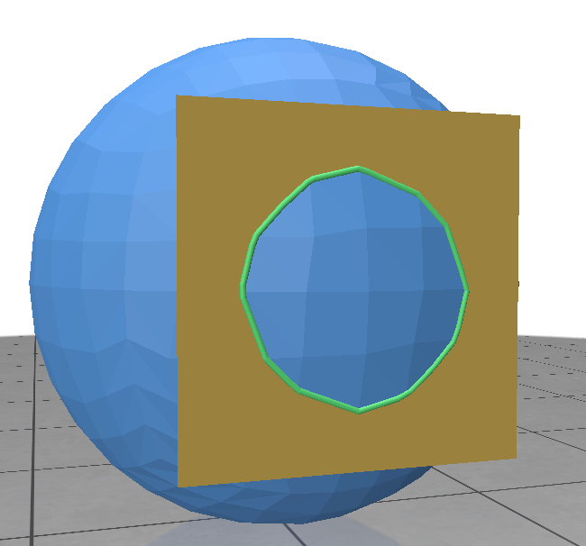
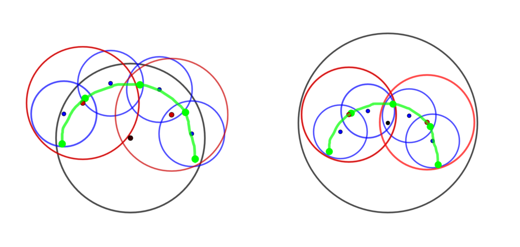
The BD-Tree works by constructing a hierarchy of minimum bounding spheres. As a first step, we need a method to construct the smallest enclosing sphere for some set of points. Fortunately, this problem has been well studied in the field of computational geometry, and we can use the randomized recursive algorithm of Welzl [3] that runs in expected linear time.
The Welzl’s algorithm is based on a simple observation: assume a minimum bounding sphere \(S\) has been computed a set of points \(P\). If a new point \(p\) is added to \(P\), then \(S\) needs to be recomputed only if \(p\) lies outside of \(S\), and the new point \(p\) must lie on the boundary of the new minimum bounding sphere for the points \(P \cup \{p\}\). So the algorithm keeps track of the set of input points and a set of support, which contains the points from the input set that must lie on the boundary of the minimum bounding sphere.
The pseudocode below [4] outlines the algorithm:
Sphere WelzlSphere(Point pt[], unsigned int numPts, Point sos[], unsigned int numSos)
{
	// if no input points, the recursion has bottomed out.
    // Now compute an exact sphere based on points in set of support (zero through four points)
	if (numPts == 0) {
		switch (numSos) {
			case 0: return Sphere();
			case 1: return Sphere(sos[0]);
			case 2: return Sphere(sos[0], sos[1]);
			case 3: return Sphere(sos[0], sos[1], sos[2]);
			case 4: return Sphere(sos[0], sos[1], sos[2], sos[3]);
		}
	}
	// Pick a point at "random" (here just the last point of the input set)
	int index = numPts - 1;
	// Recursively compute the smallest bounding sphere of the remaining points
	Sphere smallestSphere = WelzlSphere(pt, numPts - 1, sos, numSos);
	// If the selected point lies inside this sphere, it is indeed the smallest
	if(PointInsideSphere(pt[index], smallestSphere))
		return smallestSphere;
	// Otherwise, update set of support to additionally contain the new point
	sos[numSos] = pt[index];
	// Recursively compute the smallest sphere of remaining points with new s.o.s.
	return WelzlSphere(pt, numPts - 1, sos, numSos + 1);
}
The BD-Tree Method
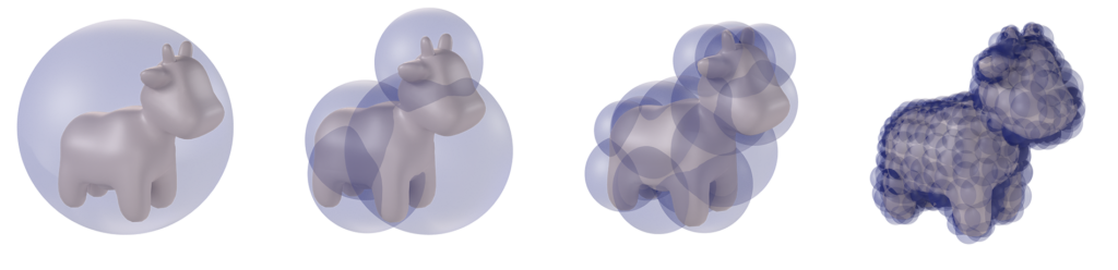
Now that we can compute the minimum bounding spheres for any set of points, we are ready to construct a hierarchical sphere tree on the undeformed model, after which it can be updated following deformation. First we note that the BD-Tree is a wrapped hierarchy, wherein the bounding spheres tightly enclose the underlying geometry but any bounding sphere at one level need not contain its child spheres. This is different from a layered hierarchy in which spheres must enclose their child spheres, but can fit the underlying geometry more loosely (see Figure 4).
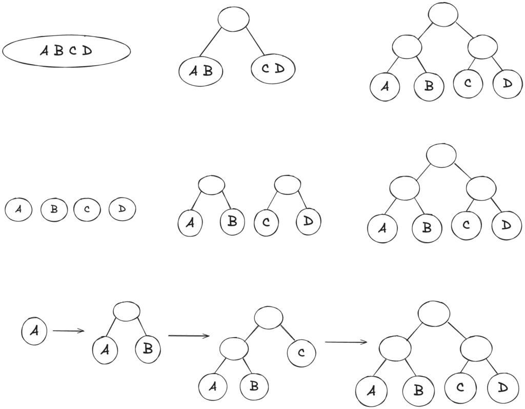
As shown in Figure 5, there are many possible approaches to building a binary tree. In our case, we use a simple top-down approach while partitioning the underlying geometry, i.e. we recursively split Spot at its median into two parts with respect to its local coordination axes, such that a leaf node (the lowest level) contains only one triangle.
As the object deforms, how do we compute the new bounding spheres quickly and efficiently?
Let \(S\) denote a sphere in the hierarchical tree with center \(c\) and radius \(R\) containing the \(k\) points of the geometry \(\{p_{i}\}_{1 \leq i \leq k}\). After the deformation, the center of the sphere \(c\) is displaced by a weighted average of the contained points’ displacements \(u_{i}\) with weights \(\beta_i\) e.g. \(\beta_i := 1/k\) for \(1 \leq i \leq k\). So the new center can be expressed as
\(\displaystyle c’ = c + \sum_{i = 1}^{k} \beta_i u_i.\)
Using the displacement equation above, we can write \(u_i\) as the sum \(\sum_{j = 1}^{r} U_{ij} q_{j}\) and substitute this into the previous equation to obtain:
\(\displaystyle c’ = c + \sum_{j = 1}^{r} \left(\sum_{i = 1}^{k} \beta_i U_{ij}\right) q_j = c + \bar{U} \boldsymbol{q}.\)
To compute the new radius \(R’\), we make use of the triangle inequality
\(\displaystyle \max_{i = 1, \dots, k} || p’_{i} – c’_{i} ||_{2} \leq \max_{i = 1, \dots, k} \left(||p’_{i}||_{2} + ||c’_{i}||_{2} \right).\)
Expanding both \(p’_{i}\) and \(c’_{i}\) using their displacement equations and re-arranging the terms, we get that
\(\displaystyle R’ = R + \sum_{j = 1}^{r} \left( \max_{i = 1, \dots, k} ||U_{ij} – \bar{U}_{j}||_{2} \right) |q_j|.\)
Thus, we have an updated bounding sphere \(S’\) with its center \(c’\) and radius \(R’\) computed as functions of the reduced coordinates \(\boldsymbol{q}\).
References
[1] Hang Si. TetGen, a Delaunay-based quality tetrahedral mesh generator. ACM Transactions on Mathematical Software, 41(2), 2015.
[2] Doug L. James and Dinesh K. Pai. BD-Tree: Output-Sensitive Collision Detection for Reduced Deformable Models. ACM Transactions on Graphics, 23(3), 2004.
[3] Emo Welzl. Smallest enclosing disks (balls and ellipsoids). New Results and New Trends in Computer Science, 555, 1991.
[4] Christer Ericson. Real-Time Collision Detection. CRC Press, Taylor & Francis Group. Chapter 4, p. 99-100. 2005.