Categories
Math Research

Redundant SDFs

Fellows: Aniket Rajnish, Ashlyn Lee, Megan Grosse, Taylor
Mentors: Ishit Mehta, Sina Nabizadeh

Repository: https://github.com/aniketrajnish/Redundant-SDFs

1.0 Problem Statement

Signed Distance Functions (SDFs) are widely used in computer graphics for rendering and animation. They provide an implicit representation of shapes, which can be converted to explicit representations using methods such as Marching Cubes (MC) and, more recently, Reach for the Spheres (RfS) [Sellan et al. 2023]. However, as we will demonstrate later in this blog post, SDFs have certain limitations in representing various types of surfaces, which can affect the quality of the resulting explicit representations.

Vector Distance Functions (VDFs) [Gomes and Faugeras, 2003] offer a promising alternative, with the potential to overcome some of these limitations. VDFs extend the concept of SDFs by incorporating directional information, allowing for more accurate representation of complex geometries.

This study explores both SDF and VDF-based reconstruction methods, comparing their effectiveness and identifying scenarios where each approach excels. By examining these techniques in detail, we aim to provide insights into their respective strengths and weaknesses, guiding future applications in computer graphics and geometric modeling.

2.0 Reconstruction from SDF

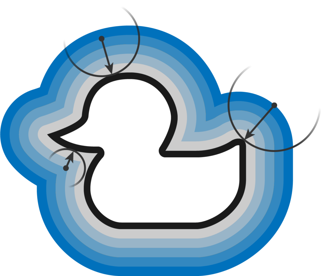
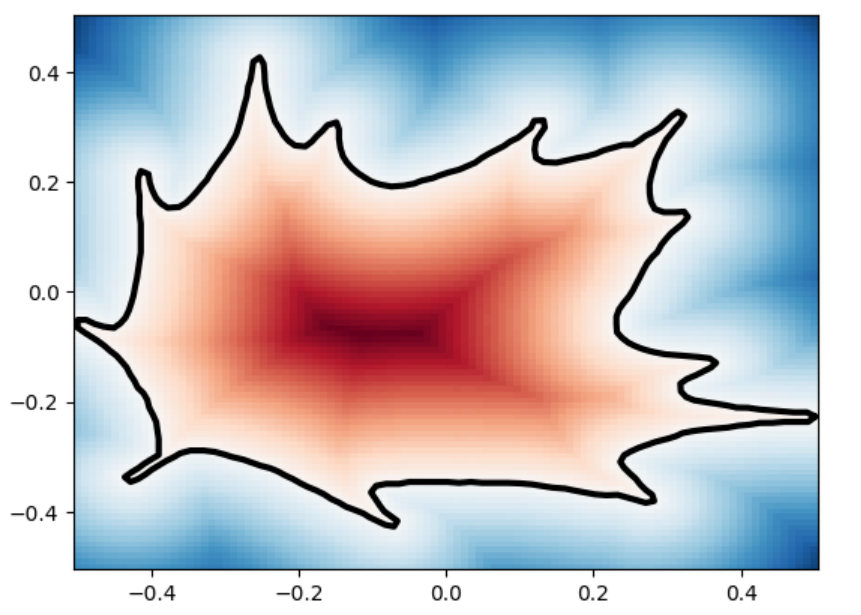
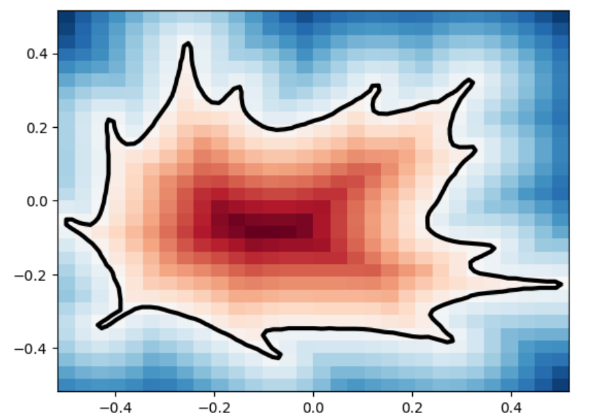
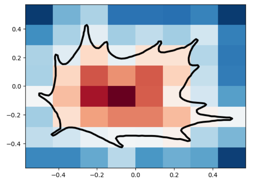
SDFs are one method of representing a surface implicitly. They involve assigning a scalar value to a set of points in a volume. The sign  of the SDF value indicates whether the point is inside (-ve) or outside (+ve) the shape, while the magnitude represents the distance to the nearest point on the surface

Mathematically, an SDF \(f(x)\) for a surface \(S\) can be defined as:

$$
f(x) = \begin{cases} -\min_{y \in S} |x – y| & \text{if } x \text{ is inside } S\\
0 & \text{if } x \text{ is on } S\\
\min_{y \in S} |x – y| & \text{if } x \text{ is outside } S \end{cases}
$$

Where, \(|x-y|\) denotes the Euclidean distance between points \(x\) and \(y\).

2.1 Extracting SDF

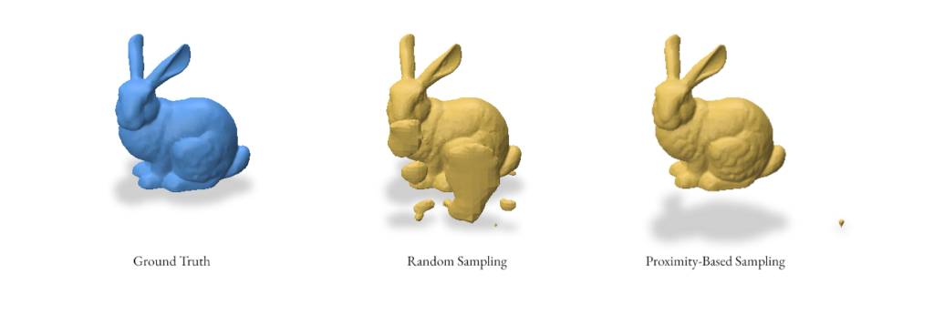
To reconstruct a surface from an SDF, we first need to obtain SDF values for a set of points in space. There are two main approaches we’ve implemented for sampling these points:

  • Random Sampling – Generating uniformly distributed random points within a bounding box that encompasses the mesh. This ensures a broad coverage of the space but may miss fine details of the surface.
  • Proximity-based Sampling – Generating points near the surface of the mesh. This method provides a higher density of samples near the surface, potentially capturing more detail. We implement this by first sampling the points and then adding Gaussian noise to these points.
def extract_sdf(sample_method: SampleMethod, mesh, num_samples=1250000, batch_size=50000, sigma=0.1):
    v, f = gpy.read_mesh(mesh)
    v = gpy.normalize_points(v)

    bbox_min = np.min(v, axis=0)
    bbox_max = np.max(v, axis=0)
    bbox_range = bbox_max - bbox_min    
    pad = 0.1 * bbox_range
    q_min = bbox_min - pad
    q_max = bbox_max + pad

    if sample_method == SampleMethod.RANDOM:
        P = np.random.uniform(q_min, q_max, (num_samples, 3))
    elif sample_method == SampleMethod.PROXIMITY:
        P = gpy.random_points_on_mesh(v, f, num_samples)
        noise = np.random.normal(0, sigma * np.mean(bbox_range), P.shape)
        P += noise   
    
    sdf, _, _ = gpy.signed_distance(P, v, f)

    return P, sdf

gpy.random_points_on_mesh() generates points on the mesh surface and gpy.signed_distance() computes the SDF values for the sampled points.

Here’s an example reconstruction using both random and proximity-based sampling for the bunny mesh using the Reach for the Arcs Algorithm:

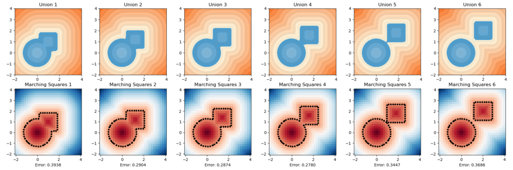
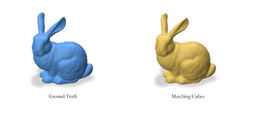
2.2 Reconstruction using Marching Cubes

Marching Cubes is a classic algorithm for extracting a polygonal mesh from an implicit function, such as an SDF. The algorithm works by dividing the space into a regular grid of cubes and then “marching” through these cubes to construct triangles that approximate the surface.

The key steps of the Marching Cubes algorithm are:

  • Divide the 3D space into a regular grid of cubes.
  • For each cube:
    • Evaluate the SDF at each of the 8 vertices.
    • Determine which edges of the cube intersect the surface (where the SDF changes sign).
    • Calculate the exact intersection points on the edges using linear interpolation.
    • Connect these intersection points to form triangles based on a predefined table of cases.

How we implement the marching cubes algorithm in our project:

def marching_cubes(self, grid_res=128):
    bbox_min = np.min(self.pts, axis=0)
    bbox_max = np.max(self.pts, axis=0)
    bbox_range = bbox_max - bbox_min
    bbox_min -= 0.1 * bbox_range
    bbox_max += 0.1 * bbox_range

    dims = (grid_res, grid_res, grid_res)
    x, y, z = np.meshgrid(
        np.linspace(bbox_min[0], bbox_max[0], dims[0]),
        np.linspace(bbox_min[1], bbox_max[1], dims[1]),
        np.linspace(bbox_min[2], bbox_max[2], dims[2]),
        indexing='ij'
    )

    grid_pts = np.column_stack((x.ravel(), y.ravel(), z.ravel()))
    self.grid_sdf = griddata(self.pts, self.sdf, grid_pts, method='linear', fill_value=np.max(self.sdf))
    self.grid_sdf = self.grid_sdf.reshape(dims)

    verts, faces, _, _ = measure.marching_cubes(self.grid_sdf, level=0)
    verts = verts * (bbox_max - bbox_min) / (np.array(dims) - 1) + bbox_min

    return verts, faces

In this implementation:

  • We first define a bounding box that encompasses all sample points.
  • We create a regular 3D grid within this bounding box.
  • We interpolate SDF values onto this regular grid using scipy.interpolate.griddata.
  • We use the skimage.measure.marching_cubes function to perform the actual Marching Cubes algorithm.
  • Finally, we scale and translate the resulting vertices back to the original coordinate system.

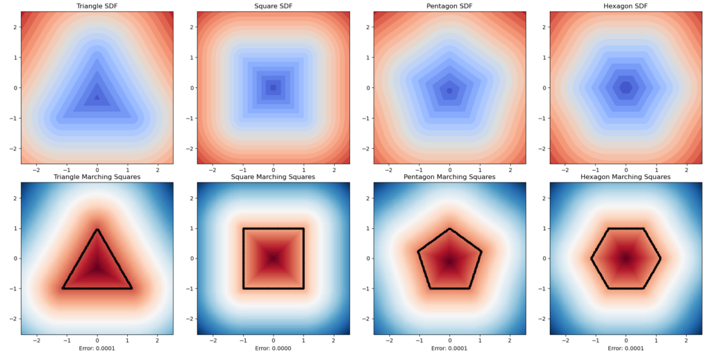
The Marching Cubes algorithm uses a look-up table to determine how to triangulate each cube based on the sign of the SDF at its vertices. There are 256 possible configurations, which can be reduced to 15 unique cases due to symmetry.

One limitation of the Marching Cubes algorithm is that it can miss thin features or sharp edges due to the fixed grid resolution. Higher resolutions can capture more detail but at the cost of increased computation time and memory usage.

In the next sections, we’ll explore more advanced reconstruction techniques that aim to overcome some of these limitations.

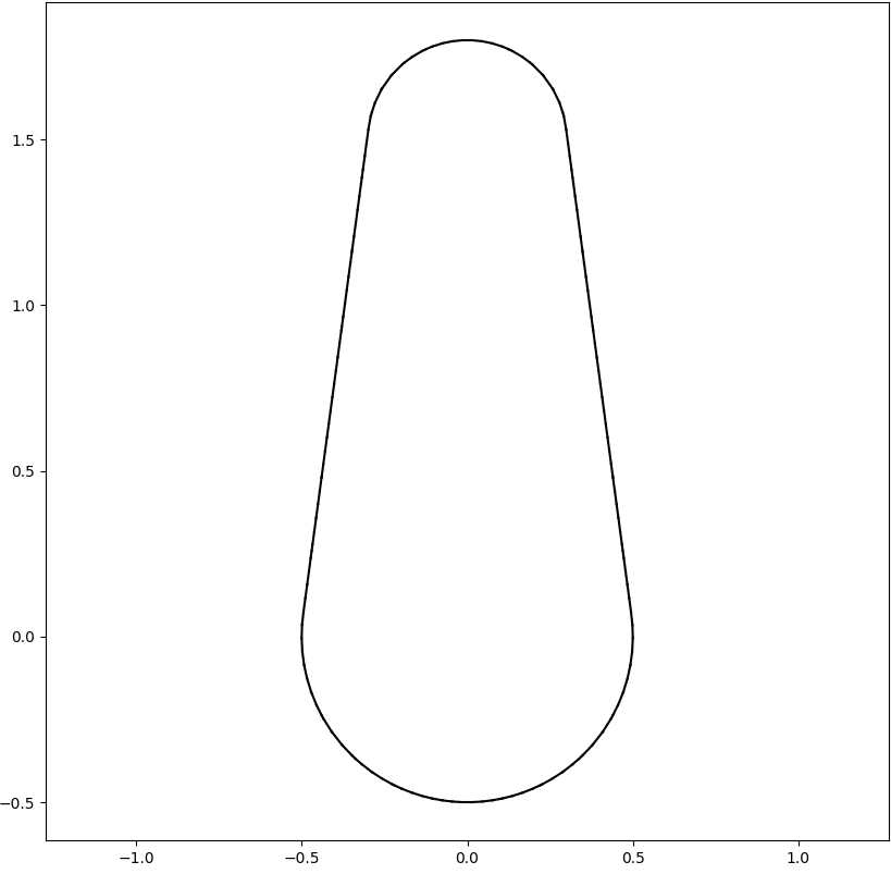
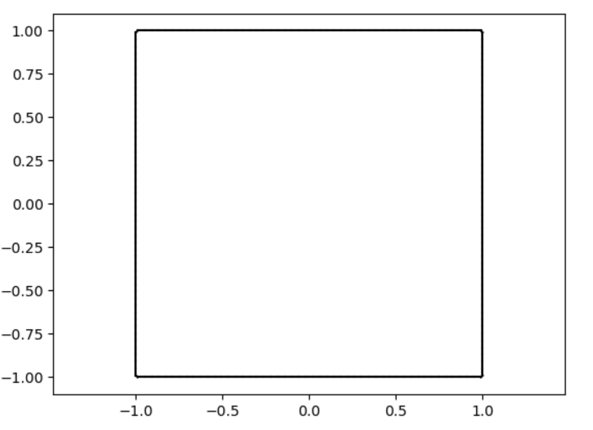
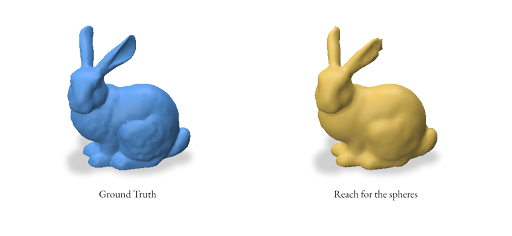
2.3 Reconstruction using Reach for the Spheres

Reach for the Spheres (RFS) is a surface reconstruction method introduced by Sellan et al. in 2023. Unlike Marching Cubes, which operates on a fixed grid, RFS iteratively refines an initial mesh to better approximate the surface represented by the SDF. The key idea behind RFS is to use local sphere approximations to guide the mesh refinement process.

The key steps of the RFS  algorithm are:

  • Start with an initial mesh (typically a low-resolution sphere).
  • For each vertex in the mesh:
    • Compute the local reach (maximum sphere radius that doesn’t intersect the surface elsewhere).
    • Move the vertex to the center of this sphere.
  • Refine the mesh by splitting long edges and collapsing short ones.
  • Repeat steps 2-3 for a fixed number of iterations or until convergence.

For a vertex \(v\) and its normal \(n\), the local reach \(r\) is computed as:

$$
r = \arg\max_{r > 0} { \forall p \in \mathbb{R}^3 : |p – v| < r \Rightarrow f(p) > -r }
$$

Where \(f(p)\) is the SDF value at point \(p\). The new position of the vertex is then:

$$v_{new} = v + r \cdot n$$

How we implement the RFS algorithm in our project:

def reach_for_spheres(self, num_iters=5):
    v_init, f_init = gpy.icosphere(2)
    v_init = gpy.normalize_points(v_init)

    sdf_func = lambda x: griddata(self.pts, self.sdf, x, method='linear', fill_value=np.max(self.sdf))

    for _ in range(num_iters):
        v, f = gpy.reach_for_the_spheres(self.pts, sdf_func, v_init, f_init)
        v_init, f_init = v, f

    return v, f

In this implementation:

  • We start with an initial icosphere mesh with the subdivision level set to 2 which gives us  162 vertices and 320 faces.
  • We define an SDF function using interpolation from our sampled points.
  • We iteratively apply the reach_for_the_spheres function from the gpytoolbox library.
  • The resulting vertices and faces are used as input for the next iteration.

Based on empirical observations, we’ve found that the best results are achieved when the number of faces and vertices in the initial icosphere is close to, but slightly less than, the expected output mesh complexity. Keeping it greater just simply results in the icosphere as the output.

Subdivision Level (n)VerticesFaces
01220
14280
2162320
36421280
425625120
51024220480
64096281920
Subdivision levels of an icosphere and corresponding vertex and face counts generated using the gpy.icosphere function.

Advantages of RFS:

  • Adaptive resolution: RFS naturally adapts to surface features, using smaller spheres in areas of high curvature and larger spheres in flatter regions.
  • Feature preservation: The method is better at preserving sharp features compared to Marching Cubes
  • Topology handling: RFS can handle complex topologies and thin features more effectively than grid-based method.

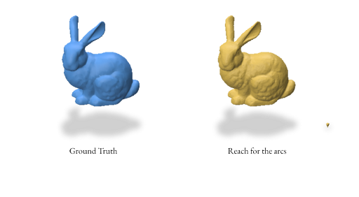
2.4 Reconstruction using Reach for the Arcs

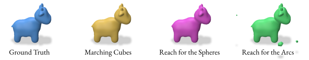
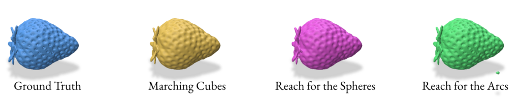
When reconstructing a mesh with Reach for the Arcs (RFA), this algorithm allows us to generate a mesh from a signed distance function. This method is a sort of extension of Reach for the Spheres in the way that it is focused on the curvature of our initial mesh as the focus for the reconstruction.  As mentioned in the paper, the run time is slower than reconstructing using Reach for the Sphere but it produces better outputs for closed surfaces with some curvature like spot and strawberry models in Section 2.5.

The key difference between RFA & RFS:

  • Instead of spheres, we use circular arcs to approximate the local surface.
  • The algorithm considers the principal curvatures of the surface when determining the arc parameters.
  • RFA includes additional steps for handling thin features and self-intersections.

For a vertex \(v\) with normal \(n\) and principal curvatures \(\kappa_1\) and \(\kappa_2\), the local arc is defined by:

$$ v(t) = v + r(\cos(t) – 1)n + r\sin(t)d $$

Where \(r = 1/\max(|\kappa_1|, |\kappa_2|)\) is the arc radius, and \(d\) is the direction of maximum curvature.

How we implement the RFA algorithm in our project:

def reach_for_arcs(self, **kwargs):
    return gpy.reach_for_the_arcs(
        self.pts, self.sdf,
        rng_seed=kwargs.get('rng_seed', 3452),
        fine_tune_iters=kwargs.get('fine_tune_iters', 3),
        batch_size=kwargs.get('batch_size', 10000),
        screening_weight=kwargs.get('screening_weight', 10.0),
        local_search_iters=kwargs.get('local_search_iters', 20),
        local_search_t=kwargs.get('local_search_t', 0.01),
        tol=kwargs.get('tol', 0.0001)
    )

This implementation uses the reach_for_the_arcs function from the gpytoolbox library. The key parameters are:

  • fine_tune_iters: Number of iterations for fine-tuning the mesh
  • batch_size: Number of points to process in each batch
  • screening_weight: Weight for the screening term in the optimization
  • local_search_iters and local_search_t: Parameters for the local search step.

Advantages of RFA:

  • Improved handling of high curvature: The use of arcs allows for better approximation of highly curved surfaces.
  • Better preservation of thin features: RFA includes specific steps to handle thin features that might be missed by RFS.
  • Reduced self-intersections: The algorithm includes checks to prevent self-intersections in the reconstructed mesh.

2.5 Validation of SDF reconstruction methods

For the validation we used the following params while performing the SDF based reconstruction:

  • SDF Computation
    • Method: SDFMethod.SAMPLE (sampling points)
    • Sampling Method: SampleMethod.PROXIMITY (sample points around the mesh surface)
    • Batch Size: 50000 (earlier we were extracting SDF in batches)
    • Sigma: 0.1 (for gaussian noise)
  • Marching Cubes
    • Grid resolution: 128 x 128 x 128
  • Reach for The Spheres
    • Number of Iterations: 10
    • Initial mesh: Icosphere with subdivision level 4 (2562 verts & 5120 faces)
  • Reach for The Arcs
    • Fine-tune iterations: 3
    • Batch size: 10,000
    • Screening weight: 10
    • Local search iterations: 20
    • Local search step size: 0.01
    • Tolerance: 0.0001

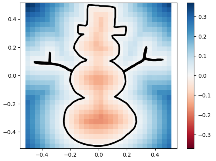
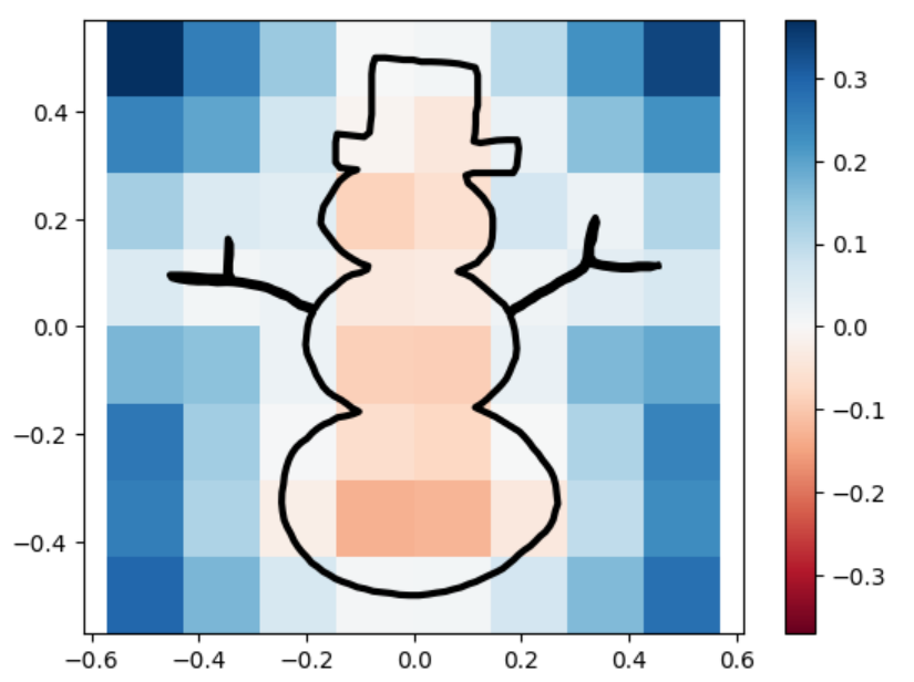
3.0 Reconstruction using VDF (Vector Distance Functions)

Reconstructions using Vector Distance Functions (VDFs) are similar to those using SDFs, except we have added a directional component. After creating a grid of points in a space, we can construct a vector stemming from each point that is both pointing in the direction that minimizes the distance to the mesh, as well as has the magnitude of the SDF at that point. In this way, the tip of each vector will lie on the real surface. From here, we can extract a point cloud of points on the surface and implement a reconstruction method.

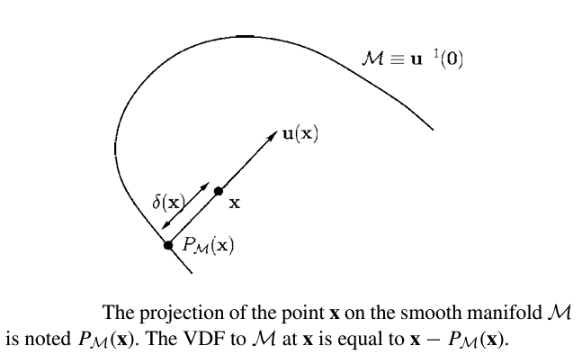
Mathematically, VDF can be used for arbitrary smooth maniform \(M\) with \(k\) dimension.

The following proof is from Gomes and Faugeras’ 2003 paper:

Given a smooth manifold \(M\), which is a subset of \(\mathbb{R}^n\), for every point \(x\), \(\delta(x)\) is that distance of \(\textbf{x}\) to \(M\). Let \(\textbf{u(x)}\) be the vector length of \(\delta(x)\), since \(u(x) = \delta{(x)}D\delta{(x)}\) for \(||D\delta{x}||\)=1. At a point \(\textbf{x}\) where \(\delta \) is differeientable, let \(\textbf{y} = P_{M}(x)\) be an unique projection of \(\textbf{x}\) onto \(M\). This point is such that \(\delta(x) = || x-y||\). Assuming \(M\) is smooth at \(y\), \(\textbf{x-y}\) is normal to \(M\) and parallel to \(D\delta{(x)}\).

Thus:

$$
\textbf{u(x)}= \textbf{x-y}= x-P_{M}(x)
$$

Advantages of VDFs:

Due to their directional nature, VDFs have the potential to have more versatility and accuracy compared to SDFs.

There are four main benefits of using VDFs instead of SDFs:

  • VDFs can be used with shapes with arbitrary codimension.
  • VDFs perform better mesh reconstruction for closed surfaces.
  • VDFs can represent open surfaces that SDFs cannot.
  • VDFs can represent non-manifold surfaces like a Möbius strip.

Disadvantages of VDFs:

Despite these advantages, VDFs do have some drawbacks:

  • VDFs require more information to be known compared to SDFs
    • SDFs only need one number (distance) associated with each point in the grid
    • VDFs, on the other hand, require three numbers (assuming a 3D grid) associated with each point, representing the x, y, and z directions associated with each vector
  • VDFs can be harder to visualize/debug compared to SDFs
  • Depending on the method used to obtain them, VDFs can be inaccurate at some grid points
    • For example, singularities in the gradient can create issues when attempting to use the gradient for a VDF
    • These inaccurate VDFs can create inaccurate point clouds, which can result in poor reconstructions

Now, we will discuss the methods we used for creating VDFs and using them for reconstructions.

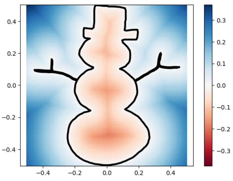
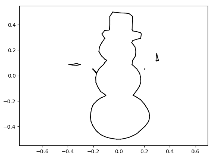
3.1 Reconstruction using Gradient

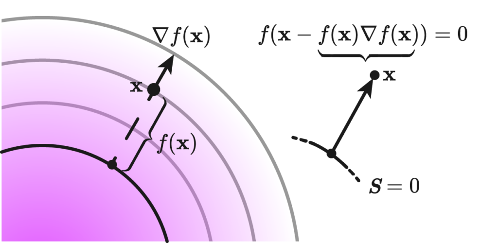
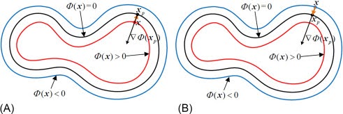
The gradient-based method leverages the fact that the gradient of a Signed Distance Function (SDF) points in the direction of maximum increase in distance. By reversing this direction and scaling by the SDF value, we obtain vectors pointing towards the surface.

Given an SDF \(\phi(x)\), the VDF \(\mathbf{u}(x)\) is defined as:

$$ \mathbf{u}(x) = -\phi(x) \frac{\nabla \phi(x)}{|\nabla \phi(x)|} $$

Where \(\nabla \phi(x)\) is the gradient of the SDF at point \(x\).

Implementation:

def compute_gradient(self):
    def finite_difference(f, axis):
        f_pos = np.roll(f, shift=-1, axis=axis)
        f_neg = np.roll(f, shift=1, axis=axis)
        f_pos[0] = f[0]  # neumann boundary condition
        f_neg[-1] = f[-1]
        return (f_pos - f_neg) / 2.0
    
    distance_grid = self.signed_distance.reshape(self.grid_shape)
    gradients = np.zeros((np.prod(self.grid_shape), 3))
    for dim in range(3):
        grad = finite_difference(distance_grid, axis=dim).flatten()
        gradients[:, dim] = grad
    
    magnitudes = np.linalg.norm(gradients, axis=1, keepdims=True)
    magnitudes = np.clip(magnitudes, a_min=1e-10, a_max=None)
    normalized_gradients = gradients / magnitudes

    signed_distance_reshaped = self.signed_distance.reshape(-1, 1)
    self.vector_distance = -1 * normalized_gradients * signed_distance_reshaped
    self.vector_distance[:, [0, 1, 2]] = self.vector_distance[:, [1, 0, 2]]

def compute_surface_points(self):
    self.vdf_pts = self.grid_vertices + self.vector_distance * self.signed_distance.reshape(-1, 1)

This method computes gradients using finite differences, normalizes them, and then scales by the SDF value to obtain the VDF. The surface points are then computed by adding the VDF to the grid vertices.

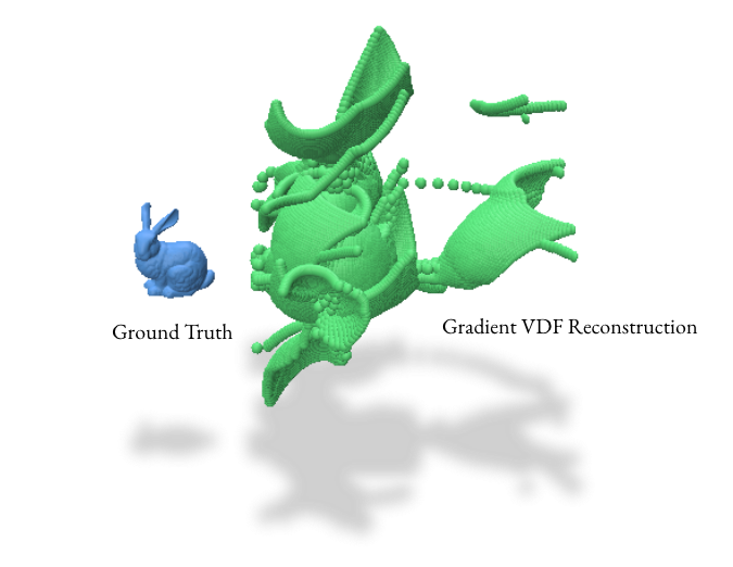
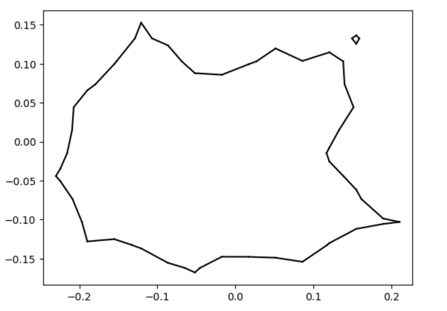
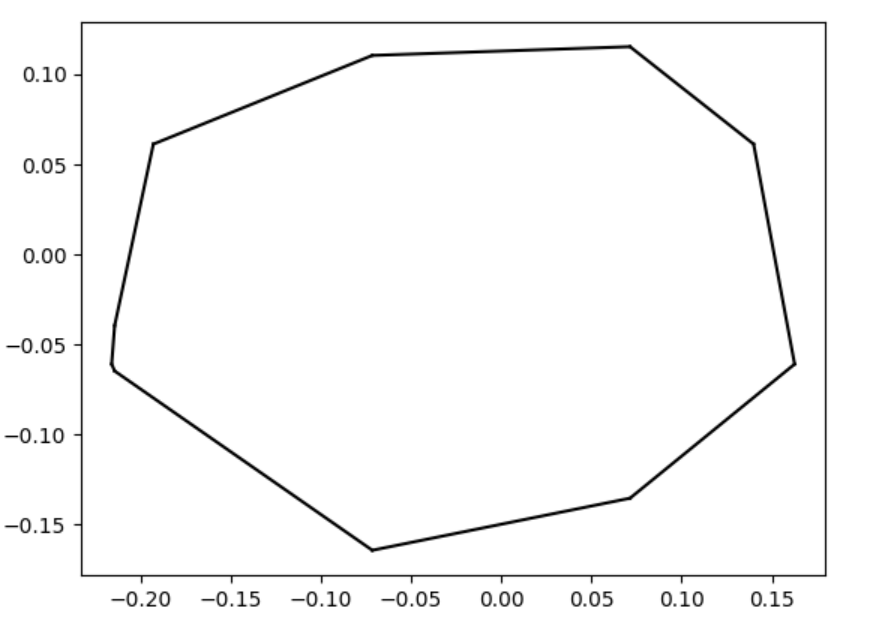
However, the gradient VDF reconstruction method, while theoretically sound, presented significant practical challenges in our experiments. As evident in the image above, this method produced numerous artifacts and distortions:.These issues likely arise from singularities and numerical instabilities in the gradient field, especially in complex geometries.

Given these results, we opted to focus on the barycentric coordinate method for our VDF reconstructions. This approach proved more robust and reliable, especially for complex 3D models with intricate surface details.

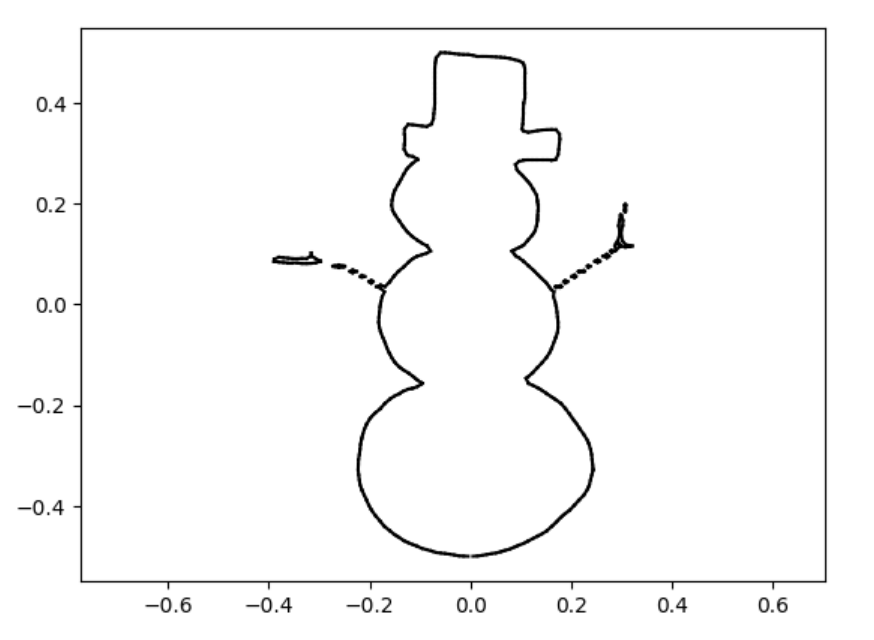
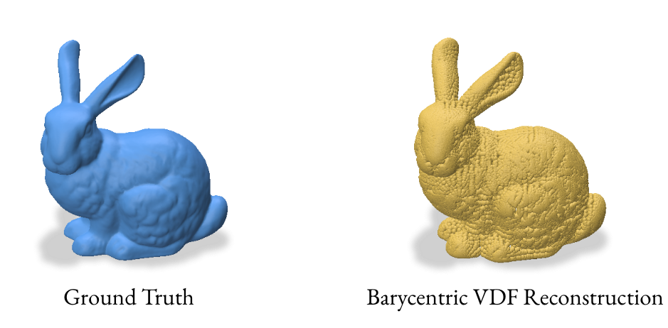
3.2 Reconstruction using Barycentric Coordinates

The barycentric coordinate method utilizes the signed_distance function from gpytoolbox to find the closest points on the mesh for each grid point. These closest points, represented in barycentric coordinates, are then converted to Cartesian coordinates to form a point cloud.

For a point \(p\) with barycentric coordinates \((u, v, w)\) relative to a triangle with vertices \((v_1, v_2, v_3)\), the Cartesian coordinates are:

$$ p = u v_1 + v v_2 + w v_3 $$

Implementation:

def compute_barycentric(self):
    self.signed_distance, self.face_indices, self.barycentric_coords = gpy.signed_distance(self.grid_vertices, self.V, self.F)
    self.vdf_pts = self.barycentric_to_cartesian()
    self.vector_distance = self.grid_vertices - self.vdf_pts
    magnitudes = np.linalg.norm(self.vector_distance, axis=1, keepdims=True)
    self.vector_distance = self.vector_distance / magnitudes

def barycentric_to_cartesian(self):
    cartesian_coords = np.zeros((self.barycentric_coords.shape[0], 3))
    face_vertex_coordinates = self.V[self.F[self.face_indices]]
    for i, (bary_coords, face_vertices) in enumerate(zip(self.barycentric_coords, face_vertex_coordinates)):
        cartesian_coords[i] = np.dot(bary_coords, face_vertices)
    return cartesian_coords

This method computes the closest points on the mesh for each grid point and converts them to Cartesian coordinates. The VDF is then computed as the normalized vector from the grid point to its closest point on the mesh.

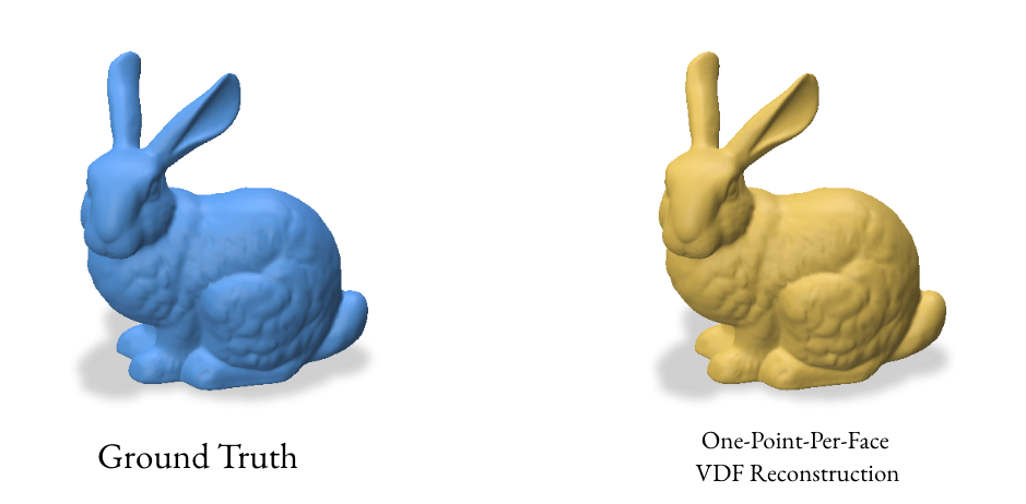
3.3 Reconstruction using one point per face

The one-point-per-face method aims to create a more uniform distribution of points on the surface by using the centroid of each face as a sample point. This approach is particularly effective for meshes with similarly-sized faces.

For a triangle face with vertices \((v_1, v_2, v_3)\), the centroid \(c\) is:

$$ c = \frac{v_1 + v_2 + v_3}{3} $$

The normal vector \(\mathbf{n}\) for the face is:

$$ \mathbf{n} = \frac{(v_2 – v_1) \times (v_3 – v_1)}{|(v_2 – v_1) \times (v_3 – v_1)|} $$

Implementation:

def compute_centroid_normal(self):
    print('Computing centroid-normal reconstruction...')
    
    def compute_triangle_centroids(vertices, faces):
        return np.mean(vertices[faces], axis=1)

    def compute_face_normals(vertices, faces):
        v0, v1, v2 = vertices[faces[:, 0]], vertices[faces[:, 1]], vertices[faces[:, 2]]
        normals = np.cross(v1 - v0, v2 - v0)
        return normals / np.linalg.norm(normals, axis=1, keepdims=True)

    centroids = compute_triangle_centroids(self.V, self.F)
    normals = compute_face_normals(self.V, self.F)

    # Double-sided representation
    self.vdf_pts = np.concatenate((centroids, centroids), axis=0)
    self.vector_distance = np.concatenate((normals, -1 * normals), axis=0)

This method computes the centroids and normals for each face of the mesh. It creates a double-sided representation by duplicating the centroids and flipping the normals, which can help in creating a watertight reconstruction.

4.0 Analyzing the Results

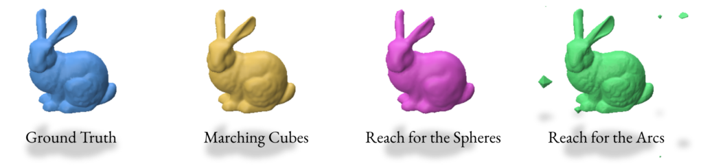
After performing various reconstruction methods using Signed Distance Functions (SDFs) and Vector Distance Functions (VDFs), it’s crucial to analyze and compare the results. This section covers the visualization, and quantitative evaluation of the reconstructed meshes.

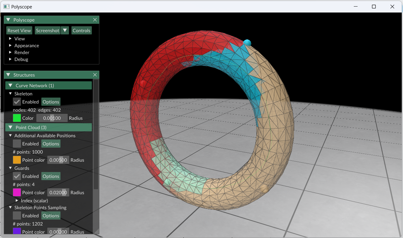
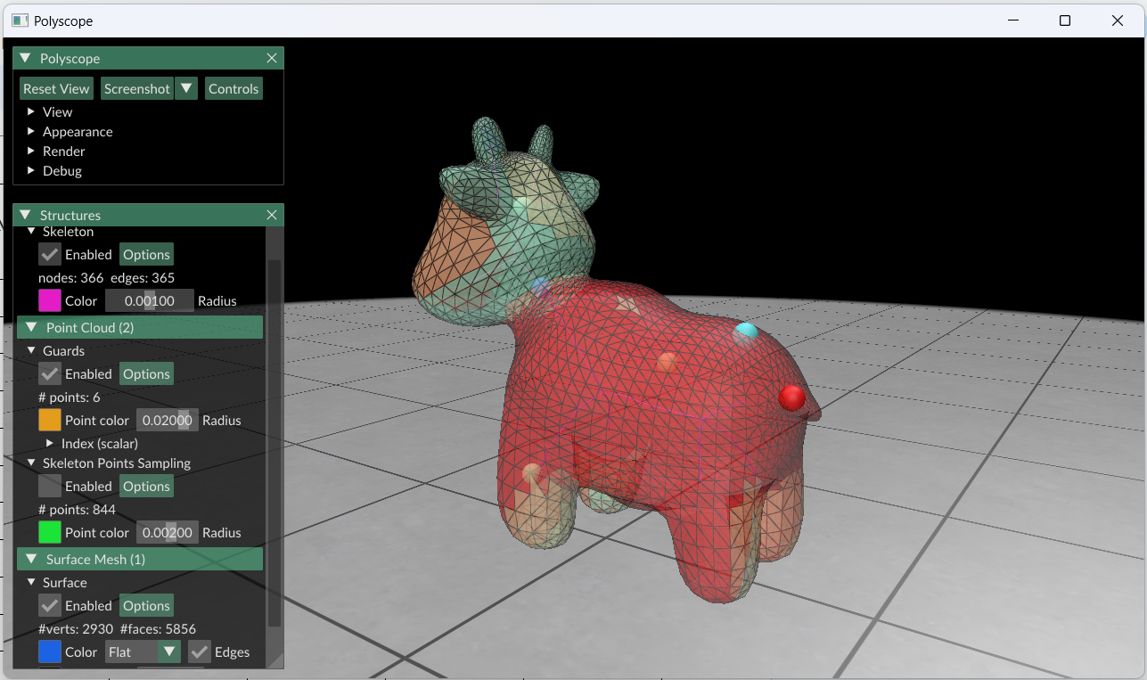
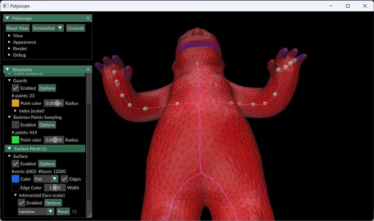
4.1 Visualizing the Results

The project uses the Polyscope library for visualizing the original and reconstructed meshes. The visualize method in all SDFReconstructor, VDFReconstructor and RayReconstructor classes handles the visualization.

This method creates a visual comparison between the original mesh and the reconstructed meshes or point clouds from different methods. The meshes are positioned side by side for easy comparison.

Additionally, the project includes a rendering functionality to export the visualization results as images. This is implemented in the render.py file

4.2 Fitness Score using Chamfer Distance

The project uses the Chamfer distance to compute a fitness score for the reconstructed meshes. The implementation is in the fitness.py file.

The Chamfer distance measures the average nearest-neighbor distance between two point sets. The fitness score is computed as:

$$\text{Fitness} = \frac{1}{1 + \text{Chamfer distance}}$$

This results in a value between 0 and 1, where higher values indicate better reconstruction.

5.0 Some Naive experimentation to get the results

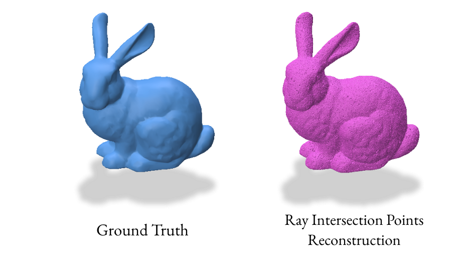
Our initial experiments with the gradient VDF method produced unexpected results due to singularities, leading to inaccurate point clouds. This prompted us to explore alternative VDF methods that directly sample points on the surface, resulting in more reliable reconstructions.

We implemented a ray-based reconstruction technique, the RayReconstructor class, as an additional method. This method generates a point cloud by shooting random rays and finding their intersections with the surface, then uses Poisson Surface Reconstruction to create the final mesh.

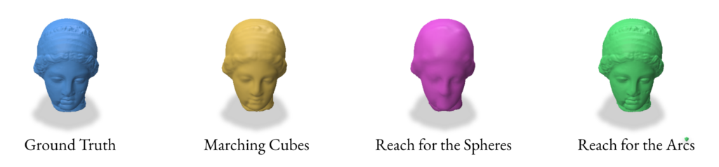
6.0 Takeaways & Further Exploration

Overall, VDFs are a promising alternative to SDFs and with the correct reconstruction method, can provide almost identical resultant meshes. They are able to provide more detail at the same resolution when compared to Marching Cubes and Reach for the Spheres. While Reach for the Arcs gives an impressive amount of detail, it often adds too much detail to where it results in details that are not present in the original mesh. VDFs, when constructed/used correctly, do not have this problem. If time permitted, we would have experimented with more non-manifold surfaces and compared the results of SDF and VDF reconstructions of these surfaces. VDFs do not require a clear outside and inside like SDFs do, so we could also explore more such surfaces manifold and non-manifold alike.

References

William E. Lorensen and Harvey E. Cline. 1987. Marching cubes: A high resolution 3D surface construction algorithm. SIGGRAPH Comput. Graph. 21, 4 (July 1987), 163–169. https://doi.org/10.11enecccevitchejdkevcjvrgvjhjhhkgcbggtkhtl45/37402.37422

Silvia Sellán, Christopher Batty, and Oded Stein. 2023. Reach For the Spheres: Tangency-aware surface reconstruction of SDFs. In SIGGRAPH Asia 2023 Conference Papers (SA ’23). Association for Computing Machinery, New York, NY, USA, Article 73, 1–11.
https://doi.org/10.1145/3610548.3618196

Silvia Sellán, Yingying Ren, Christopher Batty, and Oded Stein. 2024. Reach for the Arcs: Reconstructing Surfaces from SDFs via Tangent Points. In ACM SIGGRAPH 2024 Conference Papers (SIGGRAPH ’24). Association for Computing Machinery, New York, NY, USA, Article 23, 1–12.
https://doi.org/10.1145/3641519.3657419

José Gomes and Olivier Faugeras. The Vector Distance Functions. International Journal of Computer Vision, vol. 52, no. 2–3, 2003.
https://doi.org/10.1023/A:1022956108418

Categories
Research

A Study on Surface Reconstruction from Signed Distance Data Part 2: Error Methods

Primary mentors:  Silvia Sellán, University of Toronto and Oded Stein, University of Southern California

Volunteer assistant:  Andrew Rodriguez

Fellows: Johan Azambou, Megan Grosse, Eleanor Wiesler, Anthony Hong, Artur RB Boyago, Sara Samy

After talking about what are some of the ways to reconstruct sdfs (see part one), we now study the question of how to evaluate their performance. Two classes of error function are considered, the first more inherent to our sdf context, and the second more general in all situations. We will first show results by our old friends, Chamfer distance, Hausdorff distance, and area method (see here for example), and then introduce the inherent one.

Hausdorff and Chamfer Distance

The Chamfer distance provides an average-case measure of the dissimilarity between two shapes. It calculates the sum of the distances from each point in one set to the nearest point in the other set. This measure is particularly useful when the goal is to capture the overall discrepancy between two shapes while being less sensitive to outliers. The Chamfer distance is defined as:
$$
d_{\mathrm{Chamfer }}(X, Y):=\sum_{x \in X} d(x, Y)=\sum_{x \in X} \inf _{y \in Y} d(x, y)
$$

The Bi-Chamfer distance is an extension that considers the average of the Chamfer distance computed in both directions (from \(X\) to \(Y\) and from \(Y\) to \(X\) ). This bidirectional measure provides a more balanced assessment of the dissimilarity between the shapes:
$$
d_{\mathrm{B} \mathrm{-Chamfer }}(X, Y):=\frac{1}{2}\left(\sum_{x \in X} \inf {y \in Y} d(x, y)+\sum{y \in Y} \inf _{x \in X} d(x, y)\right)
$$

The Hausdorff distance, on the other hand, measures the worst-case scenario between two shapes. It is defined as the maximum distance from a point in one set to the closest point in the other set. This distance is particularly stringent because it reflects the largest deviation between the shapes, making it highly sensitive to outliers.

The formula for Hausdorff distance is:
$$
d_{\mathrm{H}}^Z(X, Y):=\max \left(\sup {x \in X} d_Z(x, Y), \sup {y \in Y} d_Z(y, X)\right)
$$

We analyze the Hausdorff distance for the uneven capsule (the shape on the right; exact sdf taken from there) in particular.

This plot visually compares the original zero level set (ground truth) with the reconstructed polyline generated by the marching squares algorithm at a specific resolution. The black dots represent the vertices of the polyline, showing how closely the reconstruction matches the ground truth, demonstrating the efficacy of the algorithm at capturing the shape’s essential features.

This plot shows the relationship between the Hausdorff distance and the resolution of the reconstruction. As resolution increases, the Hausdorff distance decreases, illustrating that higher resolutions produce more accurate reconstructions. The log-log plot with a linear fit suggests a strong inverse relationship, with the slope indicating a nearly quadratic decrease in Hausdorff distance as resolution improves.

Area Method for Error

Another error method we explored in this project is an area-based method. To start this process, we can overlay the original polyline and the generated polyline. Then, we can determine the area between the two, counting all regions as positive area. Essentially, this means that if we take values inside a polyline to be negative and outside a polyline to be positive, the area counted as error consists of the set of all regions where the sign of the original polyline’s SDF is not equal to the sign of the generated polyline’s SDF. The resultant area corresponds to the error of the reconstruction.

Here is a simple example of this area method using two quadrilaterals. The area between them is represented by their union (all blue area) with their intersection (the darker blue triangle) removed:

Here is an example of the area method applied to a star, with the area quantity corresponding to error printed at the top:

Inherent Error Function

We define the error function between the reconstructed polyline and the zero level set (ZLS) of a given signed distance function (SDF) as:
$$
\mathrm{Error}=\frac{1}{|S|} \sum_{s \in S} \mathrm{sdf}(s)
$$

Here, \(S\) represents a set of sample points from the reconstructed polyline generated by the marching squares algorithm, and \(|\mathrm{S}|\) denotes the cardinality of this set. The sample points include not only the vertices but also the edges of the reconstructed polyline.

The key advantage of this error function lies in its simplicity and directness. Since the SDF inherently encodes the distance between any query point and the original polyline, there’s no need to compute distances separately as required in Hausdorff or Chamfer distance calculations. This makes the error function both efficient and well-suited to our specific context, providing a more streamlined and integrated approach to measuring the accuracy of the reconstruction.

Note that one variant one can consider is to square the \(\mathrm{sdf}(s)\) part to get rid of the signed nature, because the signs can cancel with each other for the reconstructed polyline is not always entirely inside the ground truth or entirely cotains the ground truth.

Below are one experiment we did for computing using this inherent error function, the unsquared one. We let the circle sdf be fixed and let the square sdf “escape” from the circle in a constant speed of \(0.2\). That is, we used the union of a fixed circle and a square with changing position as a series of shapes to do analysis. We then draw with color map used in this repo for the ground truths and the marching square results using the common color map.

The inherent error of each union After several trials, one simple observation drawn from this escapaing motion is that when two shapes are more confounding with each other, as in the initial stage, the error is higher; and when the image starts to have two separated connected components, the error rises again. The first one can perhaps be explained by what the paper pointed out as pseudo-sdfs, and the second one is perhaps due to occurence of multipal components.

Here is another experiment. We want to know how well this method can simulate the physical characteristics of an object’s rugged level. We used a series of regular polygons. Although the result is theoretically unintheresting as the errors are all nearly zero, this is visually conformting.

Categories
Research

A Study on Surface Reconstruction from Signed Distance Data Part 1: SDFs

Primary mentors:  Silvia Sellán, University of Toronto and Oded Stein, University of Southern California

Volunteer assistant:  Andrew Rodriguez

Fellows: Johan Azambou, Megan Grosse, Eleanor Wiesler, Anthony Hong, Artur, Sara  

The definition of SDFs using ducks

Suppose that you took a piece of metal wire, twisted into some shape you like, let’s make it a flat duck, and then put it on a little pond. The splash of water made by said wire would propagate as a wave all across the pond, inside and outside the wire. If the speed of the wave were \(1 m/s \), you’d have, at every instant, a wavefront telling you exactly how far away a given point is from the wire.

This is the principle behind a distance field, a scalar valued field \( d(\mathbf{x}) \) whose value at any given point \(\mathbf{x}\) is given by \( d(\mathbf{x}, S) = \min_{\mathbf{y}}d(\mathbf{x}, \mathbf{y})\), where \( S \) is a simpled closed curve. To make this a signed distance field, we can distinguish between the interior and exterior of the shape by adding a minus sign in the interior region.

Suppose we were to define sdf without knowing the boundary \(S\); given a region \( \Omega \) and a surface \( S \), whose inside is defined as the closure of \( \overline{\Omega} = A \). A function \( f : \mathbb{R}^n \rightarrow \mathbb{R} \) is said to be a signed distance function if for every point \( \mathbf{x} \in \Omega \) , we have eikonality \( | \nabla f | = 1 \) and closest point condition:
\[ f( \mathbf{x} – f(\mathbf{x}) \nabla f(\mathbf{x})) = 0 \]

The statement reads very simply: if we have a point \( \mathbf{x} \), and take the difference vector to the normal of the level set at hand times the distance, it should take us to the point \( \mathbf{x} \) closest to the zero level set.

This second definition is equivalent to the first one by an observation that eikonality implies \(1\)-Lipschitz property of the function \(f\) and it is also used for the last step of the following derivation: \(\exists q \in S:=f^{-1}(0)\)
$$
p-f(p) \nabla f(p)=q \Longrightarrow p-q=f(p) \nabla f(p) \Longrightarrow|p-q|=|f(p)|
$$

This combined with \(1\)-Lipschitz property gives a proof of contradiction for characterization of sdf by eikonality and closest point condition.

Our project was focused on the SDF-to-Surface reconstruction methods, which is, given a SDF, how can we make a surface out of it? I’ll first tell you about the much simpler problem, which is Surface-to-SDF.

Our SDFs

To lay the foundation, we started with the 2D case: SDFs in the plane from which we can extract polylines. Before performing any tests, we needed a database of SDFs to work with. We created our SDFs using two different skillsets: art and math.

The first of our SDFs were hand-drawn, using an algorithm that determined the closest perpendicular distance to a drawn image at the number of points in a grid specified by the resolution. This grid of distance values was then converted into a visual representation of these distance values – a two-dimensional SDF. Here are some of our hand-drawn SDFs!

The second of our SDFs were drawn using math! Known as exact SDFs, we determined these distances by splitting the plane into regions with inequalities and many AND/OR statements. Each of these regions was then assigned an individual distance function corresponding to the geometry of that space. Here are some of our exact SDF functions and their extracted polylines!

Exact vs. Drawn

Exact Signed Distance Functions (SDFs) provide precise, mathematically rigorous measurements of the shortest distance from any point to the nearest surface of a shape, derived analytically for simple forms and through more complex calculations for intricate geometries. These are ideal for applications demanding high precision but can be computationally intensive. Conversely, drawn or approximate SDFs are numerically estimated and stored in discretized formats such as grids or textures, offering faster computation at the cost of exact accuracy. These are typically used in digital graphics and real-time applications where speed is crucial and minor inaccuracies in distance measurements are acceptable. The choice between them depends on the specific requirements of precision versus performance in the application.

Operations on SDFs

For two SDFs, \(f_1(x)\) and \(f_2(x)\), representing two shapes, we can define the following operations from constructive geometry:

Union
$$
f_{\cup}(x) = \min(f_1(x), f_2(x))
$$

Intersection
$$
f_{\cap}(x) = \max(f_1(x), f_2(x))
$$

Difference
$$
f_{\setminus}(x) = \max(f_1(x), -f_2(x))
$$

We used these operations to create the following new sdfs: a cat and a tessellation by hexagons.

Marching Squares Reconstructions with Multiple Resolutions

The marching_squares algorithm is a contouring method used to extract contour lines (isocontours) or curves from a two-dimensional scalar field (grid). It’s the 2D analogue of the 3D Marching Cubes algorithm, widely used for surface reconstruction in volumetric data. When applied to Signed Distance Functions (SDFs), marching_squares provides a way to visualize the zero level set (the exact boundary) of the function, which represents the shape defined by the SDF. Below are visualizations of various SDFs which we passed into marching squares with varied resolutions in order to test how well it reconstructs the original shape.

SDF / Resolution100×10030×308×8
leaf
leaf
marching_squares
uneven capsule
uneven capsule marching_squares
snowman
snowman marching_squares
square
square
marching_squares
sdfs and reconstructions in three different resolutions.

SDFs in 3D Geometry Processing

While the work we have done has been 2D in our project, signed-distance functions can be applied to 3D geometry meshes in the same way. Below are various examples from recent papers that use signed distance functions in the 3D setting. Take for example marching cubes, a method for surface reconstruction in volumetric data developed by Lorensen and Cline in 1987 that was originally motivated by medical imaging. If we start with an implicit function, then the marching cubes algorithm works by “marching” over a uniform grid of cubes and then locating the surface of interest by seeing where the surface intersects with the cubes, and adding triangles with each iteration such that a triangle mesh can ultimately be formed via the union of each triangle. A helpful visualization of this algorithm can be found here

Take for example our mentors Silvia Sellán and Oded Stein’s recent paper “Reach For the Spheres:Tangency-Aware Surface Reconstruction of SDFs” with C. Batty which introduces a new method for reconstructing an explicit triangle mesh surface corresponding to an SDF, an algorithm that uses tangency information to improve reconstructions, and they compare their improved 3D surface reconstructions to marching cubes and an algorithm called Neural Dual Contouring. We can see from their figure below that their SDF and tangency-aware and reconstruction algorithm is more accurate than marching cubes or NDCx.

(From Sellan et al, 2024) The Reach for the Spheres method that using tagency information for more accurate surface reconstructions can be seen on both 10^3 and 50^3 SDF grids as being more accurate than competing methods of marching cubes and NDCx. They used features of SDF and the idea of tangency constraints for this novel algorithm.

Another SGI mentor, Professor Keenan Crane, also works with signed distance functions. Below you can see in his recent paper “A Heat Method for Generalized Signed Distance” with Nicole Feng, they introduce a novel method for SDF approximation that completes a shape if the geometric structure of interest has a corrupted region like a hole.

(From Feng and Crane, 2024): In this figure, you can see that the inputted curves in magenta are broken, and the new method introduced by Feng and Crane works by computing signed distances from the broken curves, allowing them to ultimately generate an approximated SDF for the corrupted geometry where other methods fail to do this.

Clearly, SDFs are beautiful and extremely useful functions for both 2D and 3D geometry tasks. We hope this introduction to SDFs inspires you to study or apply these functions in your future geometry-related research. 

References

Sellán, Silvia, Christopher Batty, and Oded Stein. “Reach For the Spheres: Tangency-aware surface reconstruction of SDFs.” SIGGRAPH Asia 2023 Conference Papers. 2023.

Feng, Nicole, and Keenan Crane. “A Heat Method for Generalized Signed Distance.” ACM Transactions on Graphics (TOG) 43.4 (2024): 1-19.

Marschner, Zoë, et al. “Constructive solid geometry on neural signed distance fields.” SIGGRAPH Asia 2023 Conference Papers. 2023.

Categories
Research

The 3D Art Gallery Problem

By Ashlyn Lee, Mutiraj Laksanawisit, Johan Azambou, and Megan Grosse

Mentored by Professor Yusuf Sahillioglu and Mark Gillespie

The 2D Art Gallery Problem addresses the following question: given an art gallery with a polygonal floor plan, what is the optimal position of security guards to minimize the number of guards necessary to watch over the entirety of the space? This problem has been adapted into the 3D Art Gallery Problem, which aims to minimize the number of guards necessary to guard the entirety of a 3D polygonal mesh. It is this three-dimensional version which our SGI research team explored this past week.

In order to determine what triangular faces a given guarding point g inside of a mesh M could “see,” we defined point p ∈ M as visible to a guarding point g ∈ M if line segment gp lay entirely within M. To implement this definition, we used ray-triangle intersection: starting from each guarding point, our algorithm constructed hypothetical rays passing through the vertices of a small spherical mesh centered on the test point. Then, the first triangle in which each ray intersected was considered “visible.”

Our primary approach to solving the 3D Art Gallery Problem was greedy strategy. Using this method, we can reduce the 3D Art Gallery Problem to a set-covering problem with the set to cover consisting of all faces that make up a given triangle mesh. As part of this method, our algorithm iteratively picked the skeleton point from our sample that could “see” the most faces (as defined by ray-triangle intersection above), and then colored these faces, showing that they were guarded. It then once again picked the point that could cover the most faces and repeated this process with new colors until no faces remained.

However, it turned out that some of our mesh skeletons were not large enough of a sample space to ensure that every triangle face could be guarded. Thus, we implemented a larger sample space of guarding points, also including those outside of the skeleton but within the mesh.

Within this greedy strategy, we attempted both additive and subtractive methods of guarding. The subtractive method involved starting with many guards and removing those with lower guarding capabilities (that were able to see fewer faces). The additive method started with a single guard, placed in the location in which the most faces could be guarded. The additive method proved to be the most effective.

Our results are below, including images of guarded meshes as well as a table comparing skeleton and full-mesh sample points’ numbers of guards and times used:

Model Used

Using only points from the skeleton

(5 attempts)

Adding 1000 more random points

(5 attempts)

No. of Guards

Time Used (seconds)

No. of Guards

Time Used (seconds)

Torus

Min: 7

Max: 8

Avg: 7.2

Min: 6.174

Max: 7.223

Avg: 6.435

Min: 4

Max: 4

Avg: 4

Min: 26.291

Max: 26.882

Avg: 26.494

spot

Unsolvable

Min: 15.660

Max: 16.395

Avg: 16.041

Min: 5

Max: 6

Avg: 5.6

Min: 98.538

Max: 100.516

Avg: 99.479

homer

Unsolvable

Min: 31.210

Max: 31.395

Avg: 31.308

Unsolvable

Min: 232.707

Max: 241.483

Avg: 237.942

baby_doll

Unsolvable

Min: 70.340

Max: 71.245

Avg: 70.840

Unsolvable

Min: 388.229

Max: 400.163

Avg: 395.920

camel

Unsolvable

Min: 91.470

Max: 93.290

Avg: 92.539

Unsolvable

Min: 504.316

Max: 510.746

Avg: 508.053

donkey

Unsolvable

Min: 89.855

Max: 114.415

Avg: 96.008

Unsolvable

Min: 478.854

Max: 515.941

Avg: 488.058

kitten

Min: 4

Max: 5

Avg: 4.2

Min: 41.621

Max: 42.390

Avg: 41.966

Min: 4

Max: 5

Avg: 4.4

Min: 299.202

Max: 311.160

Avg: 302.571

man

Unsolvable

Min: 64.774

Max: 65.863

Avg: 65.200

Unsolvable (⅖)

Min: 15

Max: 15

Avg: 15

Min: 482.487

Max: 502.787

Avg: 494.051

running_pose

Unsolvable

Min: 38.153

Max: 38.761

Avg: 38.391

Unsolvable

Min: 491.180

Max: 508.940

Avg: 500.162

teapot

Min: 10

Max: 11

Avg: 10.2

Min: 39.895

Max: 40.283

Avg: 40.127

Min: 7

Max: 8

Avg: 7.8

Min: 230.414

Max: 235.597

Avg: 233.044

spider

Unsolvable

Min: 151.243

Max: 233.798

Avg: 179.692

Min: 26

Max: 28

Avg: 27

Min: 1734.485

Max: 2156.615

Avg: 1986.744

bunny_fixed

Unsolvable

Min: 32.013

Max: 44.759

Avg: 37.380

Min: 6

Max: 6

Avg: 6

Min: 274.152

Max: 347.479

Avg: 302.596

table

Min: 16

Max: 16

Avg: 16

Min: 358.471

Max: 430.318

Avg: 387.133

Min: 13

Max: 16

Avg: 15.2

Min:1607.658 

Max: 1654.312

Avg: 1627.800

lamb

Min: 13

Max: 13

Avg: 13

Min:72.651 

Max: 74.011

Avg: 73.480

Min:11 

Max: 13

Avg: 11.8

Min: 472.033

Max: 488.215

Avg: 479.064

pig

Min: 12

Max: 13

Avg: 12.4

Min:148.879 

Max: 150.889

Avg: 149.670

Min: 15

Max: 17

Avg: 16

Min: 752.750

Max: 789.704

Avg: 766.684

*Note: Unsolvable means that not all of the faces were intersected

Further Research

Given the time restraint, we were unable to explore all of the different approaches and techniques. Firstly, we would ensure all the faces were intersected as it is evident that with our current approach, some of the faces are not getting intersected. This could be applied to the code itself, or the skeleton of the mesh. We could test different approaches of skeletonization to ensure we have the optimal skeleton of the mesh when implementing these approaches. Next, we would have hoped to develop the updated subtractive approach of guarding to compare the results with both additive approaches. We would presume that the results of the runtime for each approach would differ and potentially the location of the guard points as well. Furthermore, we could compare our approaches to those from the literature to determine if we developed a more efficient approach. 

Categories
Talks

The Life and Legacy of Bui Tuong Phong

Information is attributed to Professor Theodore Kim & Dr. Yoehan Oh

Bui Tuong Phong, 1969

Today, SGI welcomed the incredible Professor Theodore Kim from Yale University, as well as postdoctoral associate Dr. Yoehan Oh, for a Zoom presentation that was just as unique as it was important. While Fellows are spending much of our time focused on the technical side of things, today we took a step back to appreciate the history of a man who deserves more appreciation. With impressive alternation between each of their slide presentations, Professor Kim and Dr. Oh discussed the far-reaching legacy—yet far-too-short life—of Bui Tuong Phong.

Bui Tuong Phong was born in 1942 in Hanoi, Vietnam, but later moved to Saigon in 1954. His history is deeply connected to the Vietnam War—known as the American War in Vietnam. During this time, herbicides with major carcinogens were sprayed in Vietnam, especially in Saigon, while he lived there. It is quite likely that he was exposed. 

Bui Tuong eventually left Saigon after being admitted to the Grenoble Institute of Technology in Grenoble, France. He later studied in Paris, and married his wife in 1969. In 1965, the Hart-Cellar Act significantly altered immigration laws in the United States, and he was able to move there. Moreover, the founding of Utah’s CS Division in 1954 provided him with additional support to begin pursuing a PhD at the University of Utah. 

After graduation, Bui Tuong taught at Stanford as an adjunct teaching fellow, before his tragically early death in 1975. His cause of death is not known for certain, but the highest possibilities are leukemia, lymphoma, or squamous cell carcinoma. It is quite likely that American war efforts in Vietnam, such as the aforementioned carcinogenic herbicides, may have contributed to his early passing.

Despite all of his efforts, Bui Tuong never got to see how much his work impacted the world. He created the famous Phong shading model and reflection algorithms. Starting with rough shading on a mesh, Bui Tuong interpolated the surface normals to smooth it out, producing a much more realistic and clean mesh. This Phong shading is now the go-to method! Phong reflection added shine in a way that 3D-animated-film-viewers had never seen before—it was satisfyingly realistic. Phong reflection proved to be rather difficult to implement because the position of the viewer’s eye is necessary. Even so, Phong reflection can be seen everywhere now–even in media as popular as Toy Story!

Despite his undeniable contributions to graphics and the entertainment industry, it seems that many are too quick to forget the man behind these contributions. Within mere years of his death, many textbooks and papers even cited his name incorrectly, confusing each of the three parts in his name. After finding such inconsistencies during their research, Professor Kim and Dr. Oh contacted Bui Tuong’s daughter and wife. They confirmed that his family name is Bui Tuong (which can also be correctly written as Bui-Tuong) and his given name is Phong. This raises some interesting questions, like why are Phong shading and reflection named after his given name? Was it Bui Tuong’s own decision, or yet another case of others not taking the time to determine Bui Tuong’s family name vs. given name? Moreover, the top search result photographs allegedly of Bui Tuong are actually not of him at all; rather, they are of an entirely different man who just happens to share Bui Tuong Phong’s given name.

In the profound-yet-saddening words of Dr. Jacinda Tran, “It’s such a cruel irony considering the legacy that [Bui Tuong Phong] left behind: he’s advanced more realistic renderings in the digital realm and yet his own personhood has been so woefully misrepresented.”

Thank you to our guest speakers today for sharing such a moving and important story—and let it be known that Bui Tuong Phong was a man robbed of many years of life, but his incredible legacy lives on.