Categories
Research

Using Bicubic Curves for a Differentiable Representation of 2D Curve Networks

SGI Fellows: Harini Rammohan, Ashlyn Lee, Diana Aldana Moreno, Ehsan Shams, Taylor Hospodarec

Project Mentor: Mikhail Bessmeltsev

SGI Volunteer: Daniel Perazzo

Raster vs Vector Images

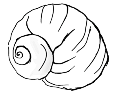
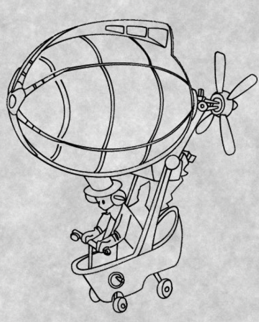
Raster and vector graphics are two fundamental types of image representations used in digital design, each with distinct characteristics and applications. A raster image is a collection of colored pixels in a bitmap, making it well-suited for capturing detailed, complex images like photographs. However, raster graphics provide no additional information about the structure of the object they represent. This limitation can be problematic in scenarios where precision and scalability are essential. For example, representing an artist’s sketch as a raster image may result in jagged curves and the loss of fine details from the original sketch. In such cases, a vector graphics representation is preferred. Unlike raster images, vector graphics use mathematical equations to define shapes, lines, and curves, allowing unlimited scalability without losing quality. This makes vector graphics ideal for logos, illustrations, and other designs where clarity and precision are crucial, regardless of size.

Bitmap and vector images on magnifying
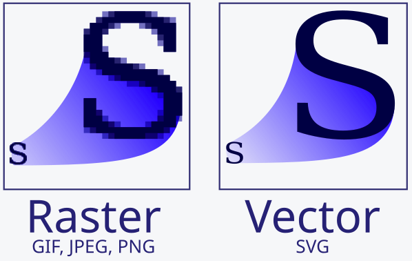
Image from https://en.wikipedia.org/wiki/Image_tracing

Bicubic Curves for Vectorization

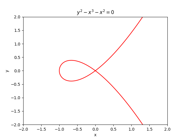
In this project, we aimed to obtain a vector graphics representation of a given sketch in raster form using bicubic curves. A bicubic curve is a polynomial of the form

{\displaystyle p(x,y)=\sum \limits _{i=0}^{3}\sum _{j=0}^{3}a_{ij}x^{i}y^{j}.}

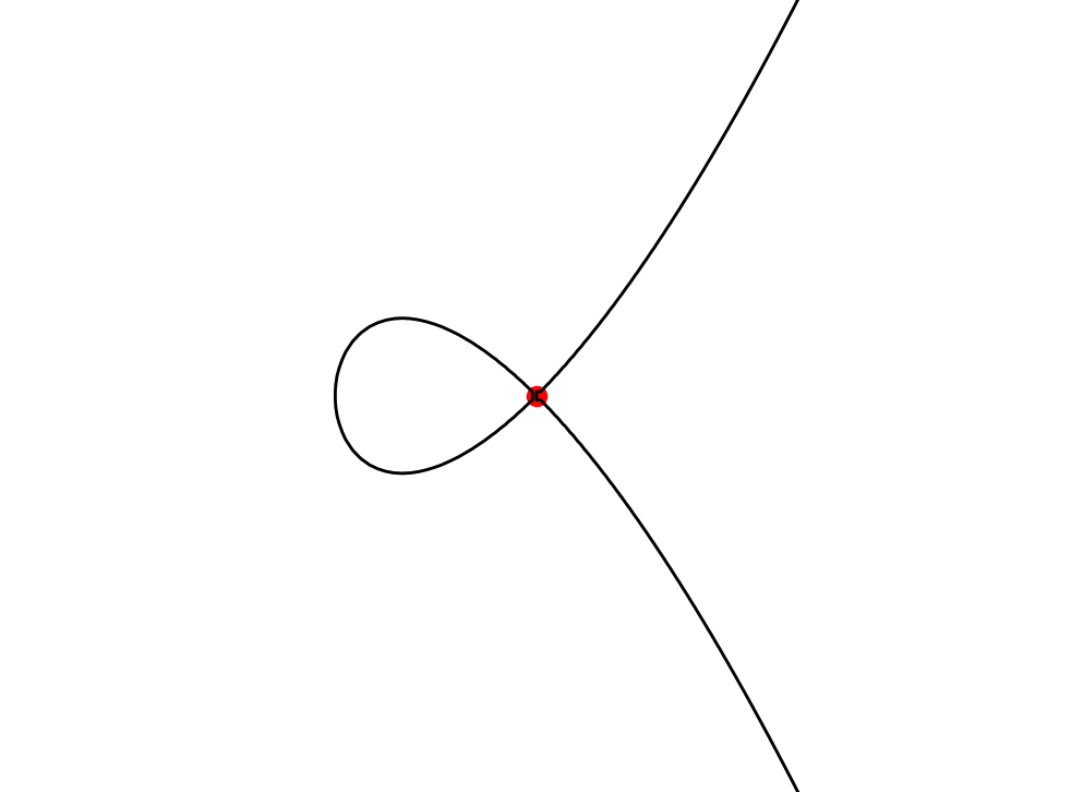
The value a bicubic function takes on a given grid cell is assumed to be uniquely determined by the value the function and its derivatives take at the vertices of the cell. Using bicubic curves allows us to more easily handle self-intersections and closed curves. Additionally, we can create discontinuities at the edges of grid cells by adding some noise to the given bicubic function. This will enable us to vectorize not only smooth but also discontinuous sketches.

A bicubic curve with a self-intersection at (0, 0)
Adding discontinuities at the grid cell edges

Preliminary Work

During the first week of the project, we implemented the following using Python:

  1. For any given grid cell, given its size and the function value p(v) as well as the derivatives px(v), py(v), and pxy(v) at each vertex v, we reconstructed and plotted the unique bicubic function satisfying these values. This reduces to solving a system of sixteen linear equations, following the steps mentioned in the “Bicubic Interpolation” Wikipedia page {4}.
  2. We added noise to the bicubic functions in each cell to create discontinuities. We also found the endpoints of curves in the grid due to the discontinuities formed above.
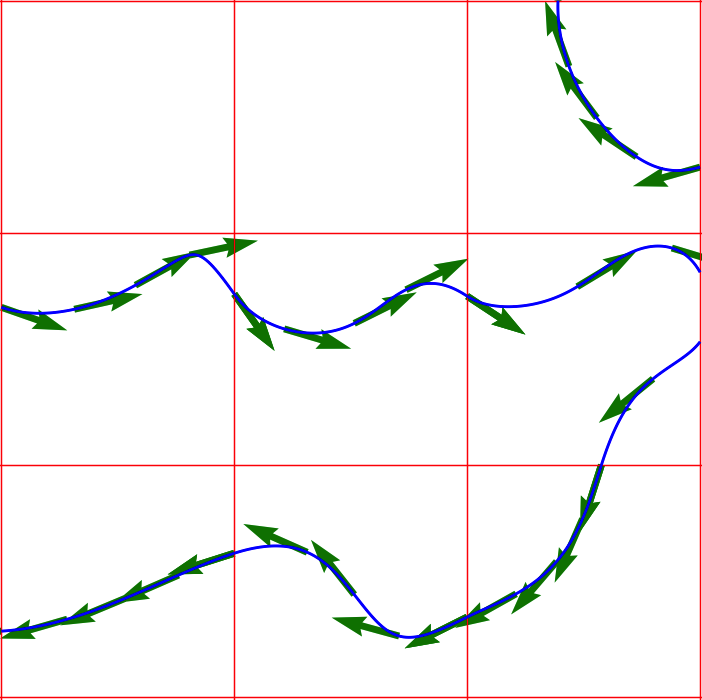
  3. At each point in the grid, we found the gradient of the bicubic functions using fsolve {5} and used them to plot the tangents at some points on the curves.
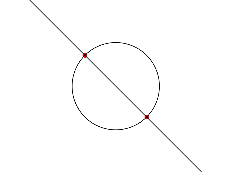
  4. We looked for self-intersections within a grid cell by finding saddle points of the bicubic function (such that the function value is 0 there). If the function is factorizable, it suffices to find the points of intersections between the 0-levels of two or more factors. Here too, we used fsolve.
Bicubic curves with tangents produced by picking four random values between -1 and 1 at each vertex

Optimization and Rendering

Vectorization

During the second week of the project, I attempted to vectorize the bitmap image by minimizing a function known as the L2 loss.

The L2 loss between the predicted and target bitmap images is computed as the sum of the squared differences for each pixel. To account for this, I gave the bicubic curves some thickness by replacing the curve Z = 0 (here Z = p(x, y) is a bicubic function) in each grid cell with the image of the function e-Z². This allowed me to determine the color at each point in the grid, defining the color of each pixel as the color at its center. Additionally, I calculated the gradient of the color at each point in a grid cell with respect to the coordinates of the corresponding bicubic curve. Using this approach, I defined the L2 loss function and its gradient as follows:

# Defining the loss function
def L2_loss(coeffs, d, width, height, x, y):
    c = np.zeros((height, width))
    for i in range(height):
        for j in range(width):
            c[i, j] = np.exp(-bicubic_function(x[j], y[i], coeffs) ** 2)
    return np.sum((c - d) ** 2)

# Derivative of c(x, y) wrt to the coeff of the x ** m * y ** n term
def colour_gradient(x, y, coeffs, m, n):
    return np.exp(-bicubic_function(x, y, coeffs) ** 2) * (-2 * bicubic_function(x, y, coeffs) * x ** m * y ** n)

# Gradient of the loss function
def gradient(coeffs, d, width, height, x, y):
    grad = np.zeros(16,)
    c = np.zeros((height, width))
    for i in range(height):
        for j in range(width):
            c[i, j] = np.exp(-bicubic_function(x[j], y[i], coeffs) ** 2)
            for n in range(4):
                for m in range(4):
                    k = m + 4 * n
                    grad[k] += 2 * (c[i, j] - d[i, j]) * colour_gradient(x[j], y[i], coeffs, m, n)
    return grad

In this code, d is the normalized numpy array of the target image and x and y are the lists of the x- and y-coordinates of the corresponding pixel centers.

Minimizing this L2 loss in each grid cell gives the vectorization that best approximates the target raster image.

Results

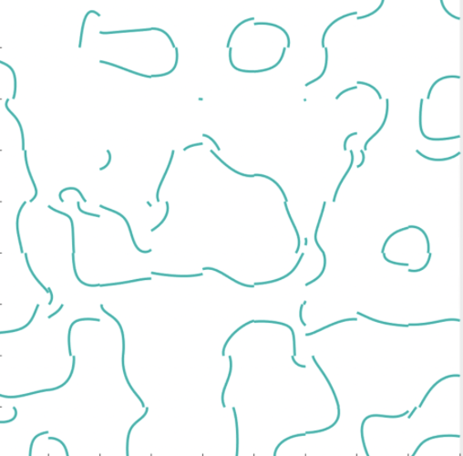
Below are some test bitmap images and their vectorized outputs.

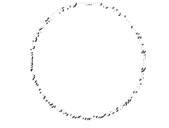
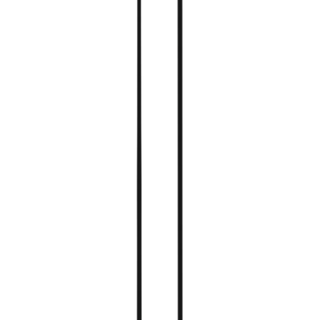
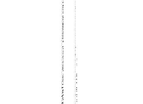
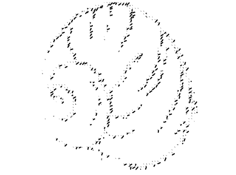
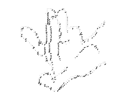
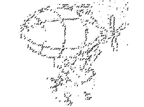
Though the curves mimic the structure of the original sketch, they are not always in the same direction as in the actual sketch. It seems like the curves assume this orientation to depict the thickness of the sketch lines.

Conclusion

Our initial plan was to utilize the code developed in the first week to create a differentiable vectorization. This approach would involve differentiating the functions we wrote to find the endpoints and intersections with respect to the coefficients of the bicubic curve. We would also use the tangents we calculated to determine the curve that best fits the original sketch.

Throughout the project, we worked with bicubic curves to ensure intersections and continuity of isolines between adjacent grid cells. However, we suspect that biquadratic curves might be sufficient for our needs and could significantly improve the implementation’s effectiveness. We are yet to confirm this and also explore whether an even lower degree might be feasible.

This project has opened up exciting avenues for future work and the potential to refine our methods further promises valuable contributions to the field. I am deeply grateful to Mikhail and Daniel for their guidance and support throughout this project.

References:

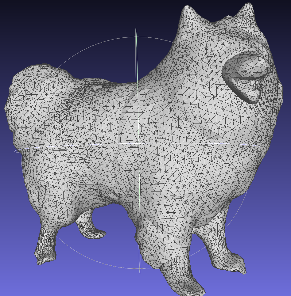
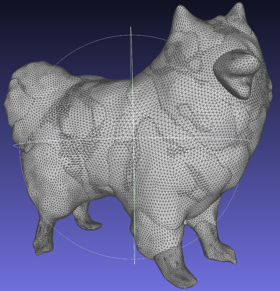
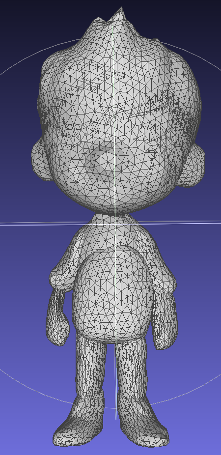
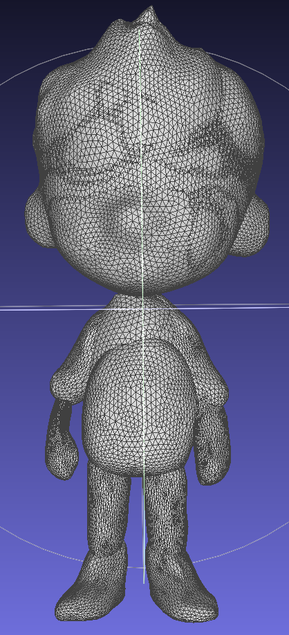
{1} Guillard, Benoit, et al. “MeshUDF: Fast and Differentiable Meshing of Unsigned Distance Field Networks”, ECCV 2022, https://doi.org/10.48550/arXiv.2111.14549

{2} Yan, Chuan, et al. “Deep Sketch Vectorization via Implicit Surface Extraction” SIGGRAPH 2024, https://doi.org/10.1145/3658197.

{3} Liu, Shichen, et al. “Soft Rasterizer: A Differentiable Renderer for Image-based 3D Reasoning” ICCV 2019, https://doi.org/10.48550/arXiv.1904.01786.

{4} “Bicubic Interpolation”. Wikipedia, https://en.wikipedia.org/wiki/Bicubic_interpolation.

{5} SciPy – fsolve (scipy.optimize.fsolve), https://docs.scipy.org/doc/scipy/reference/generated/scipy.optimize.fsolve.html

Categories
Research

Graph-based Optimal Transport for Keypoint Matching: Extending the Sinkhorn Solver

SGI Fellows: Harini Rammohan, Nicolas Pigadas, Riccardo Ali

Project Mentors: Mahdi Saleh and Dani Velikova

SGI Volunteer: Matheus Araujo

Optimal Transport and the Sinkhorn Algorithm:

Optimal Transport (OT), intuitively speaking, finds the most efficient way to transport mass from one probability distribution to another. For example, suppose the surface of a beach is given as the ambient space \(X\), and the various distributions of sand on the surface are represented by probability distributions on \(X\). Suppose also that we are given a cost function \(C:X\times X\to\mathbb{R}_{\geq 0} \), where \(C(x,y)\) represents the cost of moving a unit mass of sand from point \(x\) to point \(y\). The OT problem in this setting is to move the sand from a source distribution to a target distribution while minimizing the total transportation cost. Working with continuous distributions is often not feasible computationally, so a common approach is to discretize distributions, say by dividing the beach into a finite collection of bins and extracting an optimal transport plan for moving sand amongst this finite collection.

In the discrete case, the transportation cost can represented by a cost matrix \(C\), where \(C_{i,j}\) is the cost of moving a unit mass of sand from bin \(i\) to bin \(j\). The Wasserstein distance between two distributions is defined as the transportation cost for the minimal transport plan and can be obtained via the Sinkhorn Algorithm. Sinkhorn’s theorem states that if \(A\) is a square matrix with positive entries, then there exist two diagonal matrices \(D_1\) and \(D_2\) with positive diagonal entries such that \(T = D_1AD_2\) is doubly stochastic (all rows and columns sum to 1). The algorithm recursively rescales rows and columns of the input matrix A until it converges to the required matrix \(T\). \(T_{ij}\) returns the amount of mass that must be transported from bin \(i\) to bin \(j\) in the minimal transport plan. 

Representation of the cost matrix for the 1D problem
Image from https://alexhwilliams.info/itsneuronalblog/2020/10/09/optimal-transport/

6D Pose Estimation using the Sinkhorn Solver:

6D pose estimation refers to the process of determining the position and orientation (together called the pose) of an object (CAD) in a three-dimensional space from an image of that object. Seeing pixels as bins and pixel values as the mass of sand in that bin, the Sinkhorn algorithm can be used to find a transport plan for matching pixels in the image to points in \(\mathbb{R}^3\). However, if the object is symmetric, there may be ambiguity in its pose and one could get multiple poses that match the image. In this case, the standard Sinkhorn approach fails. Inspired by the work in the SuperGlue {1} and EPOS {2} papers, we aimed to extend the differentiable Sinkhorn solver to cases with one-to-many solutions and incorporate graph neural networks to estimate the 6D pose of such symmetric objects.

The proposed pipeline for the project
6D Object Pose Estimation
Image from Huang, Junwen, et al. “Matchu: Matching unseen objects for 6d pose estimation from rgb-d images.”CVPR. 2024

The hurdles were, first to come up with a cost matrix that best suited the problem, implement a one-to-many Sinkhorn solver from the Python OT library, and use a Perspective-N-Point {5} approach to find the pose of each of the solutions returned by the Sinkhorn solver. Another challenge was finding the correct axis of symmetry of the pose; we planned to first assume prior information about the axis of symmetry and later incorporate the problem of finding this axis itself. Unfortunately, we decided not to continue with the second week of the project and hence were not able to produce concrete results. However, a brief description of our ideas for overcoming each hurdle is given below.

Ambiguity due to symmetry
Image from Manhardt, Fabian, et al. “Explaining the ambiguity of object detection and 6d pose from visual data.” ICCV 2019.

Ideas for the Implementation:

The image was meant to be a 2D point cloud with features from which we could determine a partial 3D point cloud. One idea we had for the cost matrix, in the case where the axis of symmetry is known, was to add a symmetry-aware cost to reduce the cost for matches that are consistent with the given symmetry. We could also try to find the translation vector by inferring it from points on the axis of symmetry of the CAD and the corresponding matches in the image. Once we do this, we will have to deal with the rotation vector, which can be optimized separately using the Sinkhorn algorithm. 

The special Euclidean group (SE(3)) is the group of all combinations of rotations, reflections, and translations in \(\mathbb{R}^3\). If we have no information about the axis of symmetry, then this group forms the set of all possible 6D poses. In this case, we must find poses in SE(3) that minimize transportation costs. We could try to compare images of the CAD after applying a pose and the 2D image point cloud and reduce the distance between the two to find the possible poses of the image.

One approach to extend the existing Sinkhorn solver to get multiple solutions is first to use the existing one to get a single solution, and then find all transport matrices that have a similar cost to the one obtained. Another is to design a collection of cost matrices rather than a single one, in a way that the existing Sinkhorn solver produces multiple (and hopefully all) possible solutions. We could get this collection of matrices by applying various poses to the original CAD as before and compute the cost of going from the modified CADs to the image.

Acknowledgements:

During the one week of the project, I learned so much about optimal transport, image matching, and pose estimation. I am very grateful to our mentors who supported and guided our progress.

References:

{1} Sarlin, Paul-Edouard, et al. “SuperGlue: Learning Feature Matching with Graph Neural Networks.” CVPR, 2020, https://doi.org/10.48550/arXiv.1911.11763.

{2} Hodan, Tomas, et al. “EPOS: Estimating 6D Pose of Objects with Symmetries.” CVPR, 2020, https://doi.org/10.48550/arXiv.2004.00605.

{3} Drost, Bertram, et al. “Explaining the Ambiguity of Object Detection and 6D Pose From Visual Data.”, ICCV, 2019, https://doi.org/10.48550/arXiv.1812.00287

{4} Williams, Alex H. “A Short Introduction to Optimal Transport and Wasserstein Distance.” It’s Neuronal!, October 9, 2020. https://alexhwilliams.info/itsneuronalblog/2020/10/09/optimal-transport/.

{5} OpenCV – Perspective-n-Point (PnP) pose computation, https://docs.opencv.org/4.x/d5/d1f/calib3d_solvePnP.html


Categories
Research

Loop Subdivision for Tetsphere Splatting

SGI Fellows: Harini Rammohan, Dianlun Luo, Idil Sulo

Project Mentor: Minghao Guo

SGI Volunteer: Shanthika Naik

Introduction:

TetSphere Splatting [Guo et al., 2024] is a cutting-edge technique for high-quality 3D shape reconstruction using tetrahedral meshes. This method stands out by delivering superior geometry without relying on neural networks or post-processing. Unlike traditional Eulerian methods, TetSphere Splatting excels in applications such as single-view 3D reconstruction and text-to-3D generation.

Our project aimed to enhance TetSphere Splatting through two key improvements:

  1. Geometry Optimization: We integrated subdivision and remeshing techniques to refine the geometry optimization process, enabling the capture of finer details and better tessellation.
  2. Adaptive TetSphere Modification: We developed adaptive mechanisms for splitting and merging tetrahedral spheres, enhancing flexibility and detail in the optimization process.

Setting up the Code Base:

Our mentor, Minghao, facilitated the setup of the codebase in a cloud environment equipped with GPU support. Using a VSCode tunnel, we were able to work remotely and make modifications within the same environment. Following the instructions in the TetSphere Splatting GitHub README file, we successfully initialized the TetSpheres and executed the TetSphere Splatting process for our input images, including those of a white dog and a cartoon boy.

Geometry Optimization:

To improve the geometry optimization in TetSphere Splatting, we explored various algorithms for adaptive remeshing and subdivision. Initially, we considered parametrization-based remeshing using Centroidal Voronoi Tessellation (CVT) but opted for direct surface remeshing due to its efficiency and simplicity. For subdivision, we chose the Loop subdivision algorithm, as it is specifically designed for triangle meshes and better suited for our application compared to Catmull-Clark.

Implementing Loop Subdivision:

In the second week of the project, I worked on implementing the loop subdivision algorithm and incorporating it into the Geometry Optimization pipeline. Below is a detailed explanation of the algorithm and the method of implementation using the example of the example of the white dog mesh after TetSphere splatting.

1. Importing the required libraries, loading and initializing the mesh:

Instead of working throughout with numpy arrays, I chose to use defaultdict, a subclass of Python dictionaries to reduce the running time of the program. unique_edges defined below ensures that the list of edges doesn’t count each edge twice, once as (e1, e2) and once as (e2, e1).

import trimesh
import numpy as np
from collections import defaultdict

init_mesh = trimesh.load("./results/a_white_dog/final/final_surface_mesh.obj")
V = init_mesh.vertices
F = init_mesh.faces
E = init_mesh.edges

def unique_edges(edges): 
    sorted_edges = np.sort(edges, axis=1)
    unique_edges = np.unique(sorted_edges, axis=0)
    return unique_edges
2. Edge-Face Adjacency Mapping

This maps edges to the faces they belong to, which will later help to identify boundary and interior edges.

def compute_edge_face_adjacency(faces):
    edge_face_map = defaultdict(list)
    for i, face in enumerate(faces):
        v0, v1, v2 = face
        edges = [(min(v0, v1), max(v0, v1)),
                 (min(v1, v2), max(v1, v2)),
                 (min(v2, v0), max(v2, v0))]
        for edge in edges:
            edge_face_map[edge].append(i)
    return edge_face_map
3. Computing New Vertices:

If an edge is a boundary edge (it belongs to only one face), then the new vertex is simply the midpoint of the two vertices at the ends of the edge. If not, the edge belongs to two faces and the new vertex is found to be a weighted average of the four vertices which make the two faces, with a weight of 3/8 for the vertices on the edge and 1/8 for the vertices not on the edge. The function also produces indices for the new vertices.

(a) The weights for an interior edge; (b) the weights for a boundary edge. Image from https://www.pbr-book.org/3ed-2018/Shapes/Subdivision_Surfaces
def compute_new_vertices(edge_face_map, vertices, faces):
    new_vertices = defaultdict(list)
    i = vertices.shape[0] - 1
    for edge, facess in edge_face_map.items():
        v0, v1 = edge
        if len(facess) == 1:  # Boundary edge
            i += 1
            new_vertices[edge].append(((vertices[v0] + vertices[v1]) / 2, i))
        elif len(facess) == 2:  # Internal edge
            i += 1
            adjacent_vertices = []
            for face_index in facess:
                face = faces[face_index]
                for vertex in face:
                    if vertex != v0 and vertex != v1:
                        adjacent_vertices.append(vertex)
            v2 = adjacent_vertices[0]
            v3 = adjacent_vertices[1]
            new_vertices[edge].append(((1 / 8) * (vertices[v2] + vertices[v3]) + 
                                       (3 / 8) * (vertices[v0] + vertices[v1]), i))
    return new_vertices
4. Create a dictionary of updated vertices:

This generates updated vertices that include both old and newly created vertices.

def generate_updated_vertices(new_vertices, vertices, edges):
    updated_vertices = defaultdict(list)
    for i in range(vertices.shape[0]):
        vertex = vertices[i, :]
        updated_vertices[i].append(vertex)
    for i in range(edges.shape[0]):
        e1, e2 = edges[i, :]
        edge = (min(e1, e2), max(e1, e2))
        vertex, index = new_vertices[edge][0]
        updated_vertices[index].append(vertex)
    return updated_vertices
5. Construct New Faces:

This constructs new faces using the updated vertices. Each old face is split into four new faces.

The four child faces created, ordered such that the ith child face is adjacent to the ith vertex of the original face and the fourth child face is in the center of the subdivided face. Image from https://www.pbr-book.org/3ed-2018/Shapes/Subdivision_Surfaces
def create_new_faces(faces, new_vertices):
    new_faces = []
    for face in faces:
        v0, v1, v2 = face
        edge_0 = tuple(sorted((v0, v1)))
        edge_1 = tuple(sorted((v1, v2)))
        edge_2 = tuple(sorted((v2, v0)))

        e0 = new_vertices[edge_0][0][1]
        e1 = new_vertices[edge_1][0][1]
        e2 = new_vertices[edge_2][0][1]

        new_faces.append([v0, e0, e2])
        new_faces.append([v1, e1, e0])
        new_faces.append([v2, e2, e1])
        new_faces.append([e0, e1, e2])
    
    return np.array(new_faces)
6. Modifying Old Vertices Based on Adjacency:

First, the function compute_vertex_adjacency finds the neighbors of each vertex. Then modify_vertices weights each of the neighbor vertices of each old vertex by a weight β (defined in the code below) and weights the old vertex by 1-nβ, where n is the degree of the old vertex. It does not change the new vertices.

Computing the new position of the old vertex v. Image from https://www.pbr-book.org/3ed-2018/Shapes/Subdivision_Surfaces
def compute_vertex_adjacency(faces):
    vertex_adj_map = defaultdict(set)
    for face in faces:
        v0, v1, v2 = face
        vertex_adj_map[v0].add(v1)
        vertex_adj_map[v0].add(v2)
        vertex_adj_map[v1].add(v0)
        vertex_adj_map[v1].add(v2)
        vertex_adj_map[v2].add(v0)
        vertex_adj_map[v2].add(v1)
    return vertex_adj_map

def modify_vertices(vertices, updated_vertices, vertex_adj_map):
    modified_vertices = defaultdict(list)
    for i in range(len(updated_vertices)):
        if i in range(vertices.shape[0]):
            vertex = vertices[i,:]
            neighbors = vertex_adj_map[i]
            n = len(neighbors)
            beta = (5 / 8 - (3 / 8 + 1 / 4 * np.cos(2 * np.pi / n)) ** 2)/n
            weight_v = 1 - beta * n
            modified_vertex = weight_v * vertex
            for neighbor in neighbors:
                neighbor_point = updated_vertices[neighbor][0]
                modified_vertex += beta * neighbor_point
            modified_vertices[i].append(modified_vertex)
        else:
            modified_vertices[i].append(updated_vertices[i][0])
    return modified_vertices
7. Generating the Final Subdivided Mesh:

Now, all that is left is to collect the modified vertices and faces as numpy arrays and create the final subdivided mesh. The function loop_subdivision_iter simply applies the loop subdivision iteratively ‘n’ times, further refining the loop each time.

def create_vertices_array(modified_vertices):
    vertices_list = [modified_vertices[i][0] for i in range(len(modified_vertices))]
    return np.array(vertices_list)

def loop_subdivision(vertices, faces, edges):
    edges = unique_edges(edges)
    edge_face_map = compute_edge_face_adjacency(faces)
    new_vertices = compute_new_vertices(edge_face_map, vertices, faces)
    updated_vertices = generate_updated_vertices(new_vertices, vertices, edges)
    new_faces = create_new_faces(faces, new_vertices)
    vertex_adj_map = compute_vertex_adjacency(new_faces)
    modified_vertices = modify_vertices(vertices, updated_vertices, vertex_adj_map)
    vertices_array = create_vertices_array(modified_vertices)
    return vertices_array, new_faces

def loop_subdivision_iter(vertices, faces, n):
    def unique_edges(faces): 
            edges = np.vstack([
            np.column_stack((faces[:, 0], faces[:, 1])),
            np.column_stack((faces[:, 1], faces[:, 2])),
            np.column_stack((faces[:, 2], faces[:, 0]))
                ])
            sorted_edges = np.sort(edges, axis=1)
            unique_edges = np.unique(sorted_edges, axis=0)
            return unique_edges
    if n == 0:
        edges = unique_edges(faces)
        return loop_subdivision(V, F, E)
    else:
        edges = unique_edges(faces)
        vertices, faces = loop_subdivision(vertices, faces, edges)
        output = loop_subdivision_iter(vertices, faces, n-1)
        return output

new_V, new_F = loop_subdivision_iter(V, F, 1)
subdivided_mesh = trimesh.Trimesh(vertices=new_V, faces=new_F)
subdivided_mesh.export("./a_white_dog_subdivided.obj")

Results:

I used the above code to obtain the subdivided meshes for four input meshes – a white dog, a cartoon boy, a camel, and a horse. The results for each of these are displayed below.

Conclusion:

The project successfully enhanced the TetSphere Splatting method through geometry optimization and adaptive TetSphere modification. The implementation of Loop subdivision refined mesh detail and smoothness, as evidenced by the improved results for the test meshes. The adaptive mechanisms introduced greater flexibility, contributing to more precise and detailed 3D reconstructions.

Through this project I learned a lot about TetSphere Splatting, Geometry Optimization and Loop Subdivion. I am very grateful to Minghao and Shanthika who supported and guided us in our progress.

References:

{1} Guo, Minghao, et al. “TetSphere Splatting: Representing High-Quality Geometry with Lagrangian Volumetric Meshes”, https://doi.org/10.48550/arXiv.2405.20283

{2} Kerbl, Bernhard, et al. “3D Gaussian Splatting 
for Real-Time Radiance Field Rendering” SIGGRAPH 2023, https://doi.org/10.48550/arXiv.2308.04079.

{3} “Remeshing I”, https://graphics.stanford.edu/courses/cs468-12-spring/LectureSlides/13_Remeshing1.pdf

{4} “Subdivision”, https://www.cs.cmu.edu/afs/cs/academic/class/15462-s14/www/lec_slides/Subdivision.pdf

{5} Pharr, Matt, et al. “Physically Based Rendering: From Theory To Implementation – 3.8 Subdivision Surfaces”, https://www.pbr-book.org/3ed-2018/Shapes/Subdivision_Surfaces.