Categories
Math Tutorials

Uniform and Angle-weighted per-vertex normals in gpytoolbox

Introduction

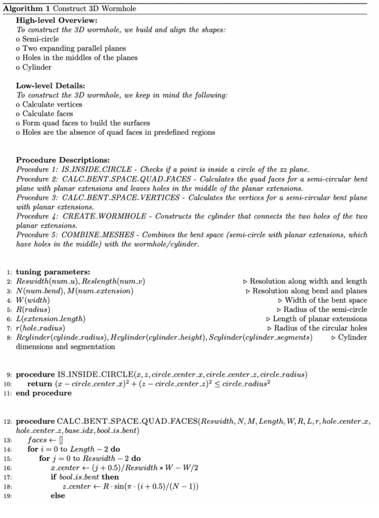
Early in the very first day of SGI, during professor Oded Stein’s great teaching sprint of the SGI introduction in Geometry Processing, we came across normal vectors. As per his slides: “The normal vector is the unit-length perpendicular vector to a triangle and positively oriented”.

Image 1: The formulas and visualisations of normal vectors in professor Oded Stein’s slides.

Immediately afterwards, we discussed that smooth surfaces have normals at every point, but as we deal with meshes, it is often useful to define per-vertex normals, apart from the well defined per-face normals. So, to approximate normals at vertices, we can average the per-face normals of the adjacent faces. This is the trivial approach. Then, the question that arises is: Going a step further, what could we do? We can introduce weights:

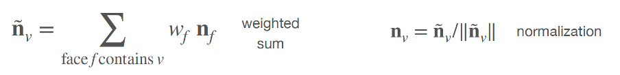
Image 2: Introducing weights to per-vertex normal vector calculation instead of just averaging the per-face normals. (image credits: professor Oded Stein’s slides)

How could we calculate them? The three most common approaches are:

1) The trivial approach: uniform weighting wf = 1 (averaging)

2)    area weighting wf = Af

3)    angle weighting wf = θf

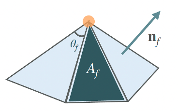
Image 3: The three most common approaches to calculating weights to perform weighted average of the per-face normals for the calculation of per-vertex normals. (image credits: professor Oded Stein’s slides)

During the talk, we briefly discussed the practical side of choosing among the various types of weights and that area weighting is good enough for most applications and, thus, this is the one implemented in gpytoolbox, a Geometry Processing python package that professor Oded Stein has significantly contributed to its development. Then, he gave us an open challenge: whoever was up for the challenge could implement the angle-weighted per-vertex normal calculation and contribute it to gpytoolbox! I was intrigued and below I give an overview of my implementation of the per_vertex_normals(V, F, weights=’area’, correct_invalid_normals=True) function.

Implementation Overview

First, I implemented an auxiliary function called compute_angles(V,F). This function calculates the angles of each face using the dot product between vectors formed by the vertices of each triangle. The angles are then calculated using the arccosine of the dot product cosine result. The steps are:

  • For each triangle, the vertices A, B, and C are extracted.
  • Vectors representing the edges of each triangle are calculated:

AB=B−A

AC=C−A

BC=C−B

CA=A−C

BA=A−B

CB=B−C

  • The cosine of each angle is computed using the dot product:

cos(α) = (AB AC)/(|AB| |AC|)

cos(β) = (BC BA)/(|BC| |BA|)

cos(γ) = (CA CB)/(|CA| |CB|)

  • At this point, the numerical issues that can come up in geometry processing applications that we discussed on day 5 with Dr. Nicholas Sharp came to mind. What if the values of arccos(angle) exceed the values 1 or -1? To avoid potential numerical problems I clipped the results to be between -1 and 1:

α=arccos(clip(cos(α),−1,1))

β=arccos(clip(cos(β),−1,1))

γ=arccos(clip(cos(γ),−1,1))

Having compute_angles, now we can explore the per_vertex_normals function. It is modified to get an argument to select weights among the options: “uniform”, “angle”, “area” and applies the selected weight averaging of the per-face normals, to calculate the per-vertex normals:

def per_vertex_normals(V, F, weights=’area’, correct_invalid_normals=True):

  1. Make sure that the V and F data structures are of types float64 and int32 respectively, to make our function compatible with any given input
  2. Calculate the per face normals using gpytoolbox
  3. If the selected weight is “area”, then use the already implemented function.
  4. If the selected weight is “angle”:
    • Compute angles using the compute_angles auxiliary function
    • Weigh the face normals by the angles at each vertex (weighted normals)
  5. Calculate the norms of the weighted normals

(A small parenthesis: The initial implementation of the function implemented the 2 following steps:

  • Include another check for potential numerical issues, replacing very small values of norms that may have been rounded to 0, with a very small number, using NumPy (np.finfo(float).eps)
  • Normalize the vertex normals: N = weighted_normals / norms

Can you guess the problem of this approach?*)

6. Identify indices with problematic norms (NaN, inf, negative, zero)

7. Identify the rest of the indices (of valid norms)

8. Normalize valid normals

9. If correct_invalid_normals == True

  • Build KDTree using only valid vertices
  • For every problematic index:
    • Find the nearest valid normal in the KDTree
    • Assign the nearest valid normal to the current problematic normal
    • Else assign a default normal ([1, 0, 0]) (in the extreme case no valid norms are calculated)

  • Normalise the replaced problematic normals

10. Else ignore the problematic normals and just output the valid normalised weighted normals

*Spoiler alert: The problem of the approach was that -in extreme cases- it can happen that the result of the normalization procedure does not have unit norm.  The final steps that follow ensure that the per-vertex normals that this function outputs always have norm 1.

Testing

A crucial stage of developing any type of software is testing it. In this section, I provide the visualised results of the angle-weighted per-vertex normal calculations for base and edge cases, as well as everyone’s favourite shape: spot the cow:

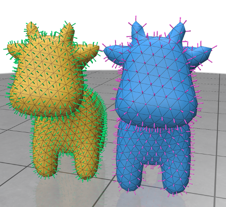
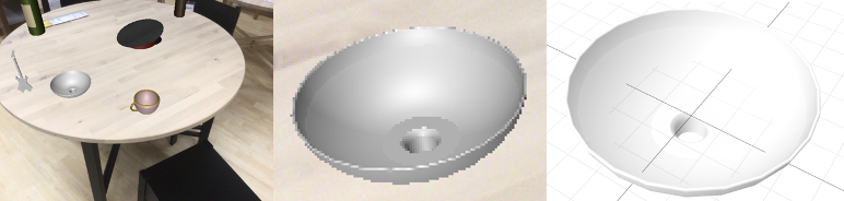
Image 4: Let’s start with spot the cow, who we all love. On the left, we have the per-face normals calculated via gpytoolbox and on the right, we have the angle-weighted per-vertex normals, calculated as analysed in the previous section.

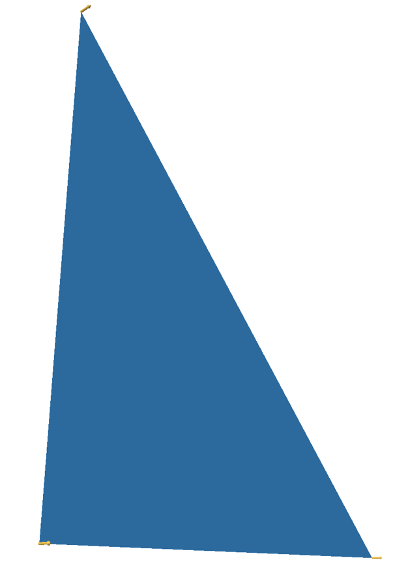
Image 5: The base case of a simple triangle.

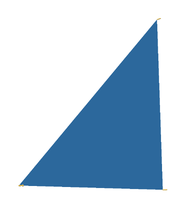
Image 6: The base case of an inverted triangle (vertices ordered in a clockwise direction)

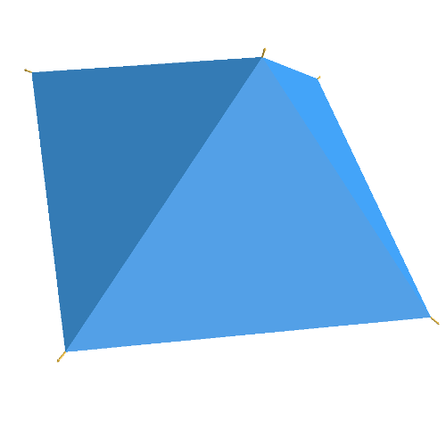
Image 7: The base case of a simple pyramid with a base.

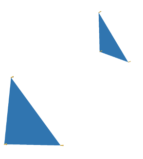
Image 8: The base case of disconnected triangles.

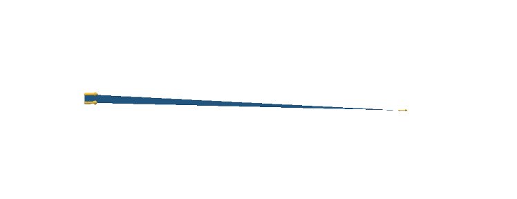
Image 9: The edge case of having a very thin triangle.

Finally, for the cases of a degenerate triangle and repeated vertex coordinates nothing is visualised. The edge cases of having very large or small coordinates have also been tested successfully (coordinates of magnitude 1e8 and 1e-12, respectively).

Having a verified visual inspection is -of course- not enough. The calculations need to be compared to ground truth data in the context of unit tests. To this end, I calculated the ground truth data via the sibling of gpytoolbox: gptoolbox, which is the respective Geometry Processing package but in MATLAB! The shape used to assert the correctness of our per_vertex_normals function, was the famous armadillo. Tests passed for both angle and uniform weights, hurray!

Final Notes

Developing the weighted per-vertex normal function and contributing slightly to such a powerful python library as gpytoolbox, was a cool and humbling experience. Hope the pull request results into a merge! I want to thank professor Oded Stein for the encouragement to take up on the task, as well as reviewing it along with the soon-to-be professor Silvia Sellán!

Categories
Math Tutorials

Wormhole II

Images: (1) The Wormhole Distance Field (DF) shape. (2) The Wormhole built using DF functions, visualized using a DF/scalar field defined over a discretized space, i.e. a grid. (3) Deploying the marching cubes algorithm (https://dl.acm.org/doi/10.1145/37402.37422) to attempt to reconstruct the surface from the DF shape. (4) Resulting surface using my reconstruction algorithm based on the principles of k-nearest neighbors (kNN), for k=10.  (5) Same, but from a different perspective highlighting unreconstructed areas, due to the DF shape having empty areas in the curved plane (see image 2 closely). If those areas didn’t exist in the DF shape, the reconstruction would have likely been exact with smaller k, and thus the representation would have been cleaner and more suitable for ML and GP tasks. (6) The reconstruction for k=5. (7) The reconstruction for k=5, different perspective.

Note: We could use a directional approach to knn for a cleaner reconstructed mesh, leveraging positional information. Alternatively, we could develop a connection correcting algorithm. Irrespectively to if we attempt the aforementioned optimizations or not, we can make the current implementation more optimized, as a lot less distances would need to be calculated after we organize the points of the DF shape based on their positions in the 3D space.

Intro

Well, SGI day 3 came… And it changed everything. In my mind at least. Silvia Sellán and Towaki Takikawa taught us -in the coolest and most intuitive ways- that there is so much more to shape representations. With Silvia, we discussed how one would expect to jump from one representation to another or even try to reconstruct the original shapes from representations that do not explicitely save connectivity information. With Towaki, we discussed Signed Distance Field (SDF) shapes among other stuff (shout out for building a library called haipera, that will definetely be useful to me) and the crazy community building crazy shapes using them. All the newfound knowledge got me thinking. Again.

Towaki was asked if there are easier/automated ways to calculate the necessary SDF functions because it would be insane to build -for e.g.- SDF cars by hand. His response? These people are actually insane! And I wanted to get a glimpse of that insanity, to figure out how to build the wormhole using Distance Field (DF) functions. Of course, my target final shape is a lot easier and it turned out that the implementation was far easier than calculating vertices and faces manually (see Wormhole I)! Then, Silvia’s words came to mind: each representation is suitable for different tasks, i.e., a task that is trivial for DF representations might be next to impossible for other representasions. So, creating a DF car is insane, but using functions to calculate the coordinates of a mesh grid car would be even more insane! Fun fact from Silvia’s slides: “The first real object ever 3D scanned and rendered was a WV Beetle by the legendary graphics researcher Ivan Sutherland’s lab (and the car belonged to his wife!)” and it was done manually:

Image (8): Calculating the coordinates of vertices and the faces to design the mesh of a Beetle manually! Geometric Processing gurus’ old school hobbies.

Method

Back to the DF Wormhole. The high-level algorithm for the DF Wormhole is attached below (for the implementation, visit this GitHub repo:

Having my DF Wormhole, the problem of surface reconstruction arose. Thankfully, Silvia had already made sure we got, not only an intuitive understanding of multiple shape representations in 2D and 3D, but also how to jump from one to another and how to reconstruct surfaces from discretized representations. It intrigued me what would happen if I used the marching cubes algorithm on my DF shape. The result was somewhat disappointing (see image 3).

Yet, I couldn’t just let it go. I had to figure out something better. I followed the first idea that came to mind: k-Neirest Neighbors (kNN). My hypothesis was that although the DF shape is in 3D, it doesn’t have any volumetric data. The hypothetical final shape is comprised by surfaces so kNN makes sense; the goal is to find the nearest neighbors and create a mechanism to connect them. It worked (see images 4, 5, 6, 7)! A problem became immediately apparent: the surface was not smooth in certain areas, but rather blocky. Thus, I developed an iterative smoothing mechanism that repositions the nodes based on the average of the coordinates of their neighbors. At 5 iterations the result was satisfying (see image 8). Below I attach the algorithm, (for the implementation, visit this GitHub repo: https://github.com/NIcolasp14/MIT_SGI-Wormhole). Case closed.

Q&A

Q: Why did I call my functions Distance Field functions (DFs) and not Signed Distance Field functions (SDFs)?

A: Because the SDF representation requires some points to have a negative value in relation to a shape’s surface (i.e., we have a negative sign for points inside the shape). In the case of the hollow shapes, such as the hollow cube and cylinder, we replace the negative signs of the inner parts of the outer shapes with positive signs, via the statement max(outer_shape, -inner_shape). Thus, our surfaces/hollow shapes only have 0 values on the surface and positive elsewhere. These type of distance fields are called unsigned (UDFs).

Q: What about the semi-cylinder?

A: The final shape of the semi-cylinder was defined to have negative values inside the radius of the semi-cylinder, 0 on the surface and positive elsewhere. But in order to remove the caps, rather than subtracting an inner cylinder, I gave them a positive value (e.g. infinity). This contradicts the definition of SDFs and UDFs, which measure distance in a continuous way. So, the semi-cylinder would be referred to as a discontinuous distance function (or continuous with specific discontinuities by design).

Future considerations

Using the smoothing mechanism and not using it has a trade off. The smooting mechanism seems to remove more faces -that we do want to have in our mesh-, than if we do not use it (see images 9, 10). The quality of the final surface certaintly depends on the initial DF shape (which indeed had empty spaces, see image 2 closely) and the hyperparameter k of kNN. Someone would need to find the right balance between the aforementioned parameters and the smoothing mechanism or even reconsider how to create the initial Wormhole DF shape or/and how to reposition the vertices, in order to smooth the surfaces more effectively. Finally, all the procedures of the algorithm can be optimized to make the code faster and more efficient. Even the kNN algorithm can be optimized: not every pair must be calculated to compare distances, because we have positional information and thus we can avoid most of the kNN calculations.

Images: (9) Mesh grid using only the mechanism that connects the k-nearest neighbors for k=5, (10) Mesh grid after the additional use of the smoothing mechanism.

Wormhole: The end

Categories
Research

Graph-based Optimal Transport for Keypoint Matching: Extended NOCs

Image 1: Our proposed solution’s pipeline, credits to our -always supportive- mentors, Saleh Mahdi and Dani Velikova!

Introduction

Our project aims to enhance Optimal Transport (OT) solvers by incorporating Graph Neural Networks (GNNs) to address the lack of geometric consistency in feature matching. The main motivation of our study is that a lot of real objects are symmetric and thus impose ambiguity. Traditional OT approaches focus on similarity measures and often neglect important neighboring information in geometric settings, proper in computer vision or graphics problems, resulting in the production of huge noise in pose estimation tasks. To tackle this problem, we hypothetize that when the object is symmetric, there are many correct matches of points around its symmetric axis and we can leverage this fact via Optimal Transport and Graph Learning.

To this end, we propose the pipeline in image 1. On a high level, we extract a 3D point cloud of an object from a 2D scene using the Normalized Object Coordinate Space (NOCs) pipeline [1], downsample the points and pool the features/NOCs embeddings of the removed points into the representative remaining points. Concurrently, we run DGCNN on the 3D ground truth mesh of the object and create a graph; this model is used as a 3D encoder [2]. We combine the aforementioned embeddings into the cost matrix used by the Sinkhorn algorithm [3], which attempts to match the points of the point cloud produced by the NOCs map with the nodes of the graph produced by the DGCNN and then to provide a symmetry estimation. We extend the differentiable Sinkhorn solver to yield one-to-many solutions; a modification we make to fully capture the symmetry of a texture-less object. In the final step, we match pairs of points and pixels and perform symmetric pose estimation via Perspective-n-Point. In this post, we study one part of our proposed pipeline, the extended NOCs, from the 2D image analysis to the extraction of the 3D point set and the pooled feature set.

Extended NOCs pipeline

Image 2: The part of the pipeline we will study in this post: Generating a 3D point cloud of a shape from a chosen 2D scene and downsampling its points. We pool the features of the removed points into remaining (seed) points.

The NOCs pipeline extracts the NOCs map and provides size and pose estimation for each object in the scene. The NOCs map encodes via colours the prediction of the normalized 3D coordinates of the target objects’ surfaces within a bounded unit cube. We extend the NOCs pipeline to create a 3D point cloud of the target object using the extracted NOCs map. We then downsample the point cloud, by fragmenting it using the Farthest Point Sampling (FPS) algorithm and only keeping the resulting seed points. In order to fully encapsulate the information extracted by the NOCs pipeline, we pool the embeddings of the nodes of each fragment into the seed points, by averaging them. This enables our pipeline to leverage the features of the target object’s 2D partial view in its scene.

Data

Images 3, 4, 5: (3) The scene of the selected symmetric and texture-less object. (4) The object in the scene zoomed in. (5) The ground truth of the object, i.e. its exact 3D model.

In order to test our hypothesis, we use an object that is not only symmetric, but also texture-less and pattern-free. The specifications of the object we use are the following:

  • Dataset: camera, val data
  • Scene: bundle 00009, scene 0001
  • Object ids: 02880940, fc77ad0828db2caa533e44d90297dd6e 
  • Link to download: https://github.com/sahithchada/NOCS_PyTorch?tab=readme-ov-file

Extended NOCs pipeline: steps visualised

In this section we visually examine each part of the pipeline and how it processes the target shape. First, we get a 2D image of a 3D scene, which is the input of the NOCs pipeline:

Image 6: The 3D scene to be analyzed.

Running the NOCs pipeline on it, we get the pose and size estimation, as well as the NOCs map for every object in the scene:

Image 7, 8: (7) Pose and size estimation of the objects in the scene. (8) NOCs maps of the objects.

The color encodings in the NOCs map encode the prediction of the normalized 3D coordinates of the target objects’ surfaces, within a bounded a unit cube. We leverage this prediction to reconstruct the 3D point cloud of our target shape, from its 2D representation in the scene. We used a statistical outlier removal method to refine the point cloud and remove noisy points. We got the following result:

Images 9, 10: (9) The 2D NOCs map of the object. (10) The 3D point cloud reconstruction of the 2D NOCs map of the target object.

The extracted 3D point cloud of the target object is then fragmented using the Farthest Point Sampling (FPS) algorithm and the seed (center/representative) points of each fragment are also calculated.

Image 11: The fragmented point cloud of the target object. Each fragment contains its corresponding seed point.

The Sinkhorn algorithm part of our project requires a lot less data points for an optimized performance. Thus, we downsample the 3D point cloud, by only keeping the seed points. In order to capture the information extracted by the NOCs pipeline, we pool the embeddings of the removed features into their corresponding seed points via averaging:

Image 12: The 3D seed point cloud. Into each seed point, we have pooled the embeddings of the removed points of their corresponding fragment.

An overview of each step and the visualised result can be seen below:

Image 13: The scene and object’s visualisation across every step of the pipeline.

Conclusion

In this study, we discussed the information extraction of a 3D object from a 2D scene. In our case, we examined the case of a symmetric object. We downsampled the resulting 3D point cloud in order for it to be effectively handled by later stages of the pipeline, but we made share to encapsulate the features of the removed points via pooling. It will be very interesting to see how every part of the pipeline comes together to predict symmetry!

At this point, I would like to thank our mentors Mahdi Saleh and Dani Velikova, as well as Matheus Araujo for their continuous support and understanding! I started as a complete beginner to these computer vision tasks, but I feel much more confident and intrigued by this domain!

Implementation

repo: https://github.com/NIcolasp14/MIT_SGI-Extended_NOCs/tree/main

References

[1] He Wang, Srinath Sridhar, Jingwei Huang, Julien Valentin, Shuran Song, and Leonidas J. Guibas. Normalized object coordinate space for category-level 6d object pose and size estimation, 2019.
[2] Yue Wang, Yongbin Sun, Ziwei Liu, Sanjay E. Sarma, Michael M. Bronstein, and Justin M. Solomon. Dynamic graph cnn for learning on point clouds, 2019.
[3] Paul-Edouard Sarlin, Daniel DeTone, Tomasz Malisiewicz, and Andrew Rabinovich. Superglue: Learning feature matching with graph neural networks. CoRR, abs/1911.11763, 2019.

Categories
Math Tutorials

Wormhole I

Images: (1) Top left: Wormhole built using Python and Polyscope with its triangle mesh, (2) Top right: Wormhole with no mesh, (3) Bottom left: A concept of a wormhole (credits to: BBC Science Focus, https://www.sciencefocus.com/space/what-is-a-wormhole), (4) A cool accident: an uncomfortable restaurant booth.

During the intense educational week that is SGI’s tutorial week, we stumbled early on, on a challenge: creating our own mesh. A seemingly small exercise to teach us to build a simple mesh, turned for me into much more. I always liked open projects that speak to the creativity of students. Creating our own mesh could be turned into anything and our only limit is our imagination. Although the time was restrictive, I couldn’t but face the challenge. But what would I choose? Fun fact about me: in my studies I started as a physicist before I switched to be an electrical and computer engineer. But my fascination for physics has never faded, so when I thought of a wormhole I knew I had to build it.

From Wikipedia: A wormhole is a hypothetical structure connecting disparate points in spacetime and is based on a special solution of the Einstein field equations. A wormhole can be visualised as a tunnel with two ends at separate points in spacetime.

Well, I thought that it would be easier than it really was. It was daunting at first -and during the development I must confess-, but when I started to break the project into steps (first principles thinking), it felt more manageable. Let’s examine the steps on a high level/top-down:

1) build a semi-circle

2) extend its both ends with lines of the same length and parallel to each other

3) make the resulting shape 3D

4) make a hole in the middle of the planes

5) connect the holes via a cylinder

And now let’s explore the bottom-up approach:

1) calculate vertices

2) calculate faces

3) form quad faces to build the surfaces

4) holes are the absence of quad faces in predefined regions

I followed this simple blueprint and the wormhole started to take shape step by step. Instead of giving the details in a never-ending text, I opt to present a high-level algorithm and the GitHub repo of the implementation.

My inspiration for this project? Two-fold; stemming from the very first day of SGI. On one hand, professor Oded Stein encouraged us to be artistic, to create art via Geometry Processing. On the other, Dr. Qingnan Zhou from Adobe shared with us 3 practical tips for us geometry processing newbies:

1) Avoid using background colours, prefer white

2) Use shading

3) Try to become an expert in one of the many tools of Geometry Processing

Well, the third stuck with me, but -of course- I am not close to becoming a master of Python for Geometric Processing and Polyscope, yet. Though, I feel like I made significant strides with this project!

I hope that this work will inspire other students to seek open challenges and creative solutions or even build upon the wormhole, refine it or maybe add a spaceship passing through. Maybe a new SGI tradition? It’s up to you!

P.S. 1: The alignment of the shapes is a little bit overengineered :).

P.S. 2: Unfortunately, it was later in the tutorial week that I was introduced to the 3DXM virtual math museum. Instead of a cylinder, the wormhole should have been a Hyperbolic K=-1 Surface of Revolution, making the shape cleaner:

Image: Hyperbolic K=-1 Surface of Revolution.