Tag: Gaussian Splatting

Project Mentors: Sainan Liu, Ilke Demir and Alexey Soupikov

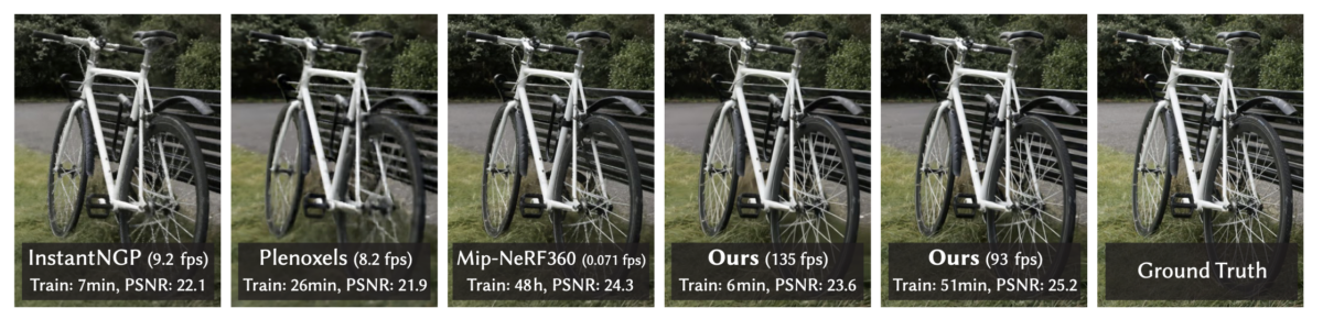
Previously, we introduced 3D Gaussian Splatting and explained how this method proposes a new approach to view synthesis. In this blog post, we will talk about how 3D Gaussian splatting [1] can be further extended to enable potential applications to reconstruct both the 3D and the dynamic (4D) world surrounding us.

We live in a 3D world and use natural language to interact with this world in our day to day lives. Until recently, 3D computer vision methods were being studied on closed set datasets, in isolation. However, our real world is inherently open set. This suggests that the 3D vision methods should also be able to extend to natural language that could accept any type of language prompt to enable further downstream applications in robotics or virtual reality.

Gaussians with Semantics

A recent trend among the 3D scene understanding methods is therefore to recognize and segment the 3D scenes with text prompts in an open-vocabulary [1,2]. While being relatively new, this problem have been extensively studied in the past year. However, these methods still investigate the semantic information within 3D scenes through an understanding point of view — So, what about reconstruction?

1. LangSplat: 3D Language Gaussian Splatting (CVPR2024 Highlight)

One of the most valuable extensions of the 3D Gaussians is the LangSplat [3] method. The aim here is to incorporate the semantic information into the training process of the Gaussians, potentially enabling a coupling between the language features and the 3D scene reconstruction process.

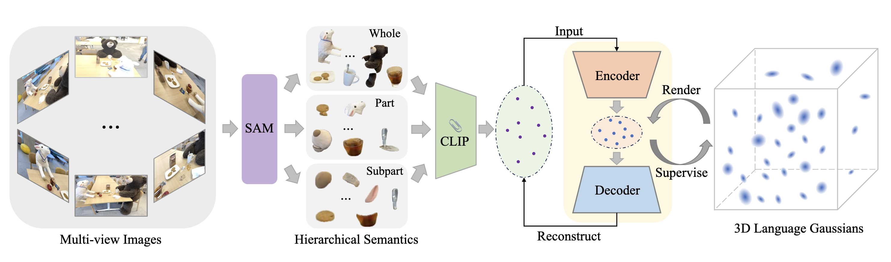
The framework of LangSplat consists of three main components which we explain below.

1.1 Hierarchical Semantics

LangSplat not only considers the objects within the scene as a whole but also learns the hierarchy to enable “whole”, “part” and “subpart”. This three levels of hierarchy is achieved by utilizing a foundation model (SAM [4]) for image segmentation. Leveraging SAM, enables precise segmentation masks to effectively partition the scene into semantically meaningful regions. The redundant masks are then removed for each of these three sets (i.e. whole, part and subpart) based on the predicted IoU score, stability score, and overlap rate between masks.

Next step is then to associate each of these masks in order to obtain pixel-aligned language features. For this, the framework makes use of a vision-language model (CLIP [5]) to extract an embedding vector per image region that can be denoted as:

$$
\boldsymbol{L}_t^l(v)=V\left(\boldsymbol{I}_t \odot \boldsymbol{M}^l(v)\right), l \in\{s, p, w\}, (1)
$$

where \(\boldsymbol{M}^l(v)\) represents the mask region to which pixel $v$ belongs at the semantic level \(l\).

The three levels of hierarchy eliminates the need for search upon querying, making the process more efficient for downstream tasks.

1.2 3D Gaussian Splatting for Language Fields

Up until now, we have talked about semantic information extracted from multi-view images mainly in 2D \(\left\{\boldsymbol{L}_t^l, \mid t=1, \ldots, T\right\}\). We can now use these embeddings to learn a 3D scene which models the relationship between 3D points and 2D pixel-aligned language features.

LangSplat aims to augment the original 3D Gaussians [1] to obtain 3D language Gaussians. Note that at this point, we have pixel aligned 512-dimensional CLIP features which increases the space-time complexity. This is because CLIP is trained on internet scale data (\(\sim\)400 million image and text pairs) and the CLIP embeddings space is expected to align with arbitrary image and text prompts. However, our language Gaussians are scene-specific which suggests that we can compress the CLIP features to enable a more efficient and scene-specific representation.

To this end, the framework trains an autoencoder trained with a reconstruction objective on the CLIP embeddings \(\left\{\boldsymbol{L}_t^l\right\}\) with L1 and cosine distance loss:

$$\mathcal{L}_{a e}=\sum_{l \in\{s, p, w\}} \sum_{t=1}^T d_{a e}\left(\Psi\left(E\left(\boldsymbol{L}_t^l(v)\right)\right), \boldsymbol{L}_t^l(v)\right), (2) $$

where \(d_{ae}(.)\) denotes the distance function used for the autoencoder. The dimensionality of the features are then reduced from \(D=512\) to \(d=3\) with high memory efficiency.

Finally, the language embeddings are optimized with the following objective to enable 3D language Gaussians:

$$\mathcal{L}_{\text {lang }}=\sum_{l \in\{s, p, w\}} \sum_{t=1}^T d_{l a n g}\left(\boldsymbol{F}_t^l(v), \boldsymbol{H}_t^l(v)\right), (3) $$

where \(d_{lang}(.)\) denotes the distance function.

1.3 Open-vocabulary Querying

The learned 3D language field can easily support open-vocabulary 3D queries, including open-vocabulary 3D object localization and open-vocabulary 3D semantic segmentation. Due to the three levels of hierarchy, each text query will be associated with three relevancy maps at each semantic level. In the end, LangSplat chooses the level that has the highest relevancy score.

Our Results

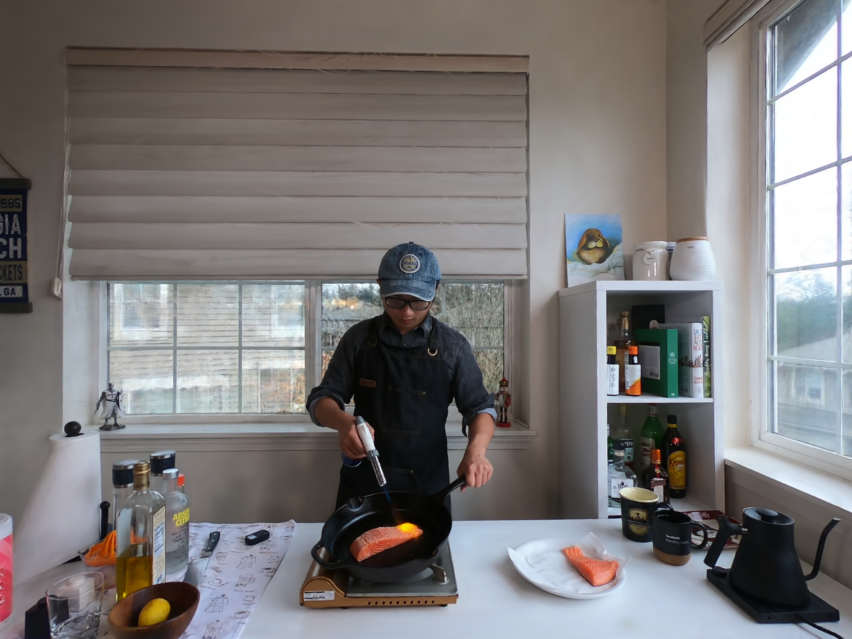
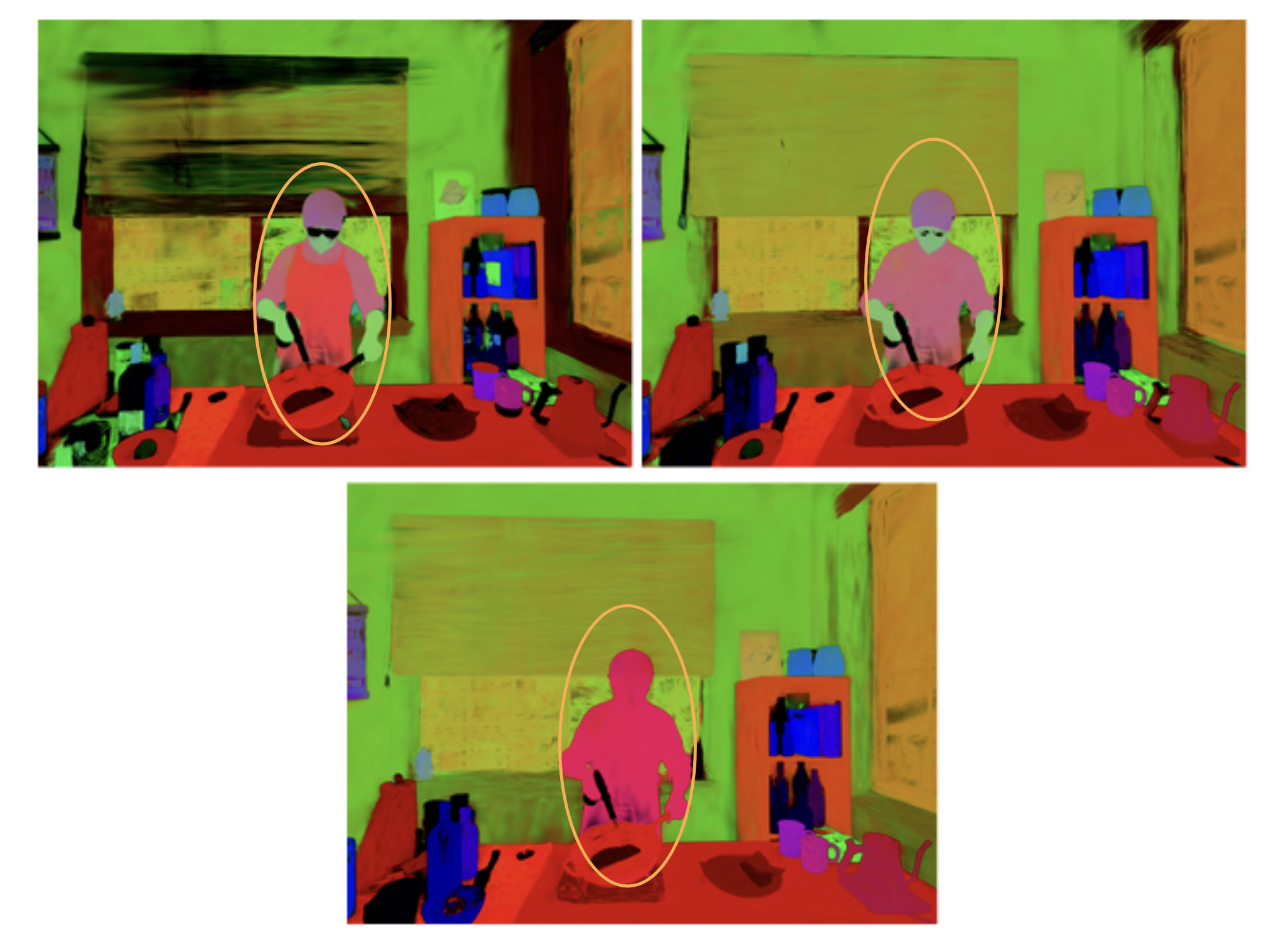
Following the previous blog post, we run LangSplat on the initial frames of the flaming salmon scene of the Neu3D dataset and share both the novel view renderings and the visualization of language features per each level of hierarchy:

Gaussians in 4D

Another extension of the 3D Gaussian splatting involves incorporating Gaussians to dynamic settings. The previously discussed dataset, Neu3D, enables a study to move from novel view synthesis for static scenes to reconstructing Free-Viewpoint Videos, or FVVs in short. The challenge here, comes from the additional time component that can pose further illumination or brightness changes. Furthermore, objects can change their look or form across time and new objects that were not present in the initial frames can later emerge in the videos. Not only this, but also the additional frames per view (1200 frames per camera view in Neu3D) highlights once again the importance of efficiency to enable further applications.

In comparison to language semantics, Gaussian splatting methods in the fourth dimension have been investigated more in detail. Before moving on with our selected method, here we highlight the most interesting works for interested readers:

• 4D Gaussian Splatting for Real-Time Dynamic Scene Rendering
• 3DGStream: On-the-Fly Training of 3D Gaussians for Efficient Streaming of Photo-Realistic Free-Viewpoint Videos
• Spacetime Gaussian Feature Splatting for Real-Time Dynamic View Synthesis

2. 3DGStream: On-the-Fly Training of 3D Gaussians for Efficient Streaming of Photo-Realistic Free-Viewpoint Videos (CVPR 2024 Highlight)

As discussed above, constructing photo-realistic FVVs of dynamic scenes is a challenging problem. While existing methods address this, they are bounded by an offline training scenario, meaning that they would require the presence of future frames in order to perform the reconstruction task. We therefore consider 3DGStream [7], due to its ability of online training.

3DGStream eliminates the requirement of long video sequences and instead performs on-the-fly construction for real-time renderable FVVs on video streams. The method consists of two main stages that involve the Neural Transformation Cache and the optimization of 3D Gaussians for the next time step.

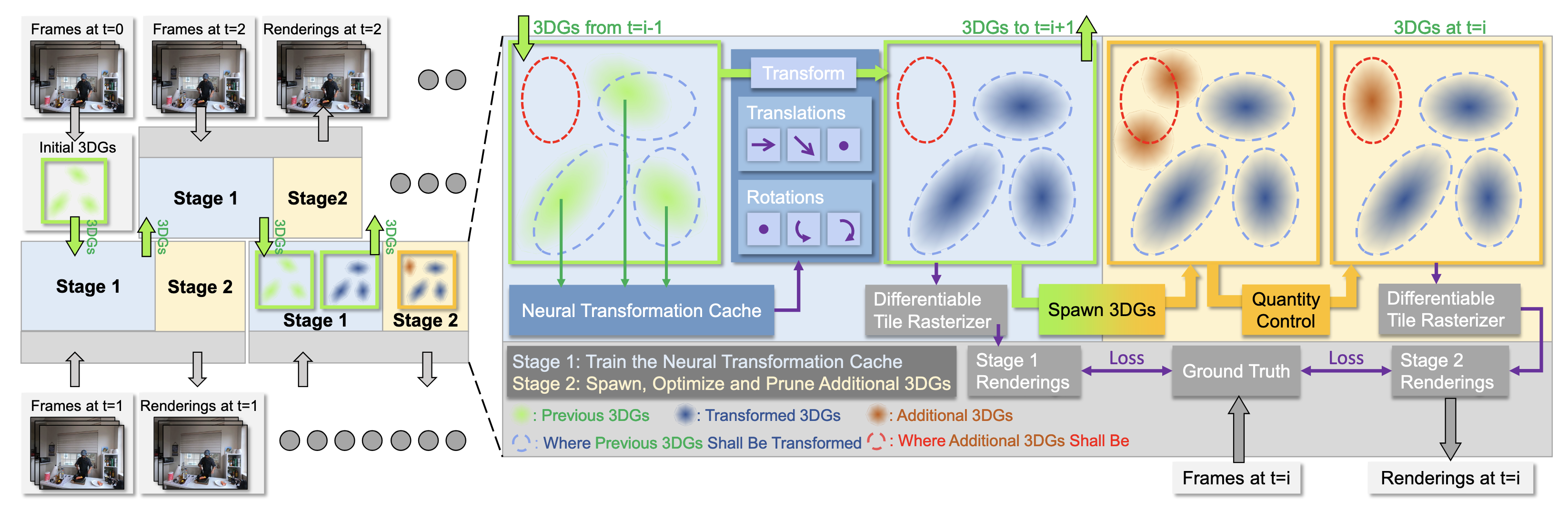
2.1 Neural Transformation Cache (NTC)

NTC enables a compact, efficient, and adaptive way to model the transformations of 3D Gaussians. Following I-NGP [8], the method uses a multi-resolution hash encoding together with a shallow fully-fused MLP. This encoding essentially uses multi-resolution voxel grids that represent the scene and the grids are mapped to a hash table storing a \(d\)-dimensional learnable feature vector. For a given 3D position \(x \in \mathcal{R}^3\), its hash encoding at resolution $l$, denoted as \(h(x; l) \in \mathcal{R}^d\), is the linear interpolation of the feature vectors corresponding to the eight corners of the surrounding grid. Then, the MLP that enhances the performance of the NTC can be formalized as

$$
d \mu, d q=M L P(h(\mu)), (4)
$$

where $\mu$ denotes the mean of the input 3D Gaussian. The mean, rotation and SH (spherical harmonics) coefficients of the 3D Gaussian are then transformed with respect to \(d\mu\) and \(dq\).

At Stage 1, the parameters of NTC are optimized following the original 3D Gaussians with \(L_1\) combined with a D-SSIM term:

$$
L=(1-\lambda) L_1+\lambda L_{D-S S I M} (5)
$$

Additionally, 3DGStream employs an additional NTC warm up which uses the loss given by:
$$
L_{w a r m-u p}=||d \mu||_1-\cos ^2(\text{norm}(d q), Q), (6)
$$
where \(Q\) is the identity quaternion.

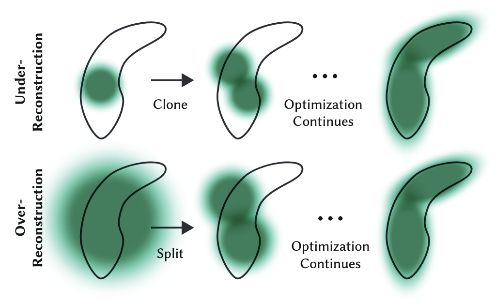
2.2 Adaptive 3D Gaussians

While 3D Gaussians transformations perform relatively well for dynamic scenes, they fall short when new objects that were not present in the initial time steps emerge later in the video. Therefore, it is essential to add new 3D Gaussians to model the new objects in a precise manner.

Based on this observation, 3DGStream aims to spawn new 3D Gaussians in regions where gradient is high. To be able to capture every region where a new object might potentially occur, the method uses an adaptive 3D Gaussian spawn strategy. To elaborate, view-space positional gradient during the final training epoch of Stage 1 is tracked, and at the end of this stage, 3D Gaussians with an average magnitude of view-space position gradients exceeding a low threshold \(\tau_{grad} = 0.00015\) are selected. For each of these selected 3D Gaussians, the position of the additional Gaussian is sampled from \(X \sim N (\mu, 2\sigma)\), where μ and Σ is the mean and the covariance matrix of the selected 3D Gaussian.

However, this may result in emerging Gaussians to quickly become transparent, failing to capture the emerging objects. To address this, SH coefficients and scaling vectors of these 3D Gaussians are derived from the selected ones, with rotations set to the identity quaternion \(q = [1, 0, 0, 0]\) with opacity 0.1. After the spawning process, the 3D Gaussians undergo an optimization utilizing the loss function (Eq. (5)) as introduced in Stage 1.

At the Stage 2, an adaptive 3D Gaussian quantity control is employed to make sure that Gaussians grow reasonably. For this reason, a high threshold of \(\tau_\alpha = 0.01\) is set for the opacity value. At the end of each epoch, new 3D Gaussians are spawned for the Gaussians where view-space position gradients exceed \(\tau_{grad}\). The spawned Gaussians inherit the rotations and SH coefficients from the original 3D Gaussians but have an adjusted scale to 80%. Finally, any 3D Gaussian with opacity values below \(\tau_{\alpha}\) are discarded to control the growth of the quantity of total number of Gaussians.

Our Results

We setup and replicate the experiments of 3DGStream on the flaming salmon scene of Neu3D.

Next Steps

To get the best of both worlds, our aim is to integrate the semantic information as in LangSplat [4] into dynamic scenes. We would like to achieve this by utilizing foundation models for videos to enable static and dynamic scene separation to construct free-viewpoint videos. We believe that this could enable further real world applications in the near future.

References

[1] Kerbl, B., Kopanas, G., Leimkühler, T., & Drettakis, G. 3D Gaussian Splatting for Real-Time Radiance Field Rendering. ACM Trans. Graph. (SIGGRAPH) 2023.
[2] Takmaz, A., Fedele, E., Sumner, R., Pollefeys, M., Tombari, F., & Engelmann, F. OpenMask3D: Open-Vocabulary 3D Instance Segmentation. NeurIPS 2024.
[3] Nguyen, P., Ngo, T. D., Kalogerakis, E., Gan, C., Tran, A., Pham, C., & Nguyen, K. Open3dis: Open-vocabulary 3d instance segmentation with 2d mask guidance. CVPR 2024.
[4] Qin, M., Li, W., Zhou, J., Wang, H., & Pfister, H. LangSplat: 3D language gaussian splatting. CVPR 2024.
[5] Kirillov, A., Mintun, E., Ravi, N., Mao, H., Rolland, C., Gustafson, L., … & Girshick, R. Segment anything. CVPR 2023.
[6] Radford, A., Kim, J. W., Hallacy, C., Ramesh, A., Goh, G., Agarwal, S., … & Sutskever, I. Learning transferable visual models from natural language supervision. ICML 2021.
[7] Sun, J., Jiao, H., Li, G., Zhang, Z., Zhao, L., & Xing, W. (2024). 3dgstream: On-the-fly training of 3d gaussians for efficient streaming of photo-realistic free-viewpoint videos. CVPR 2024.
[8] Müller, T., Evans, A., Schied, C., & Keller, A. Instant neural graphics primitives with a multiresolution hash encoding. ACM transactions on graphics (TOG) 2022.

Project Mentors: Ilke Demir, Sainan Liu and Alexey Soupikov

Among novel view synthesis methods, Neural Radiance Fields, or NeRFs, revolutionized implicit 3D scene representations by optimizing a Multi-Layer Perceptron (or MLP) using volumetric ray-marching [1]. While the continuity in these methods helps the optimization procedure, achieving high visual quality requires neural networks that are costly to train and render.

3D Gaussian Splatting for Real-Time Radiance Field Rendering

A recent work [2] addresses this issue by proposing a 3D Gaussian representation that achieves equal or better quality than the previous implicit radiance field approaches. This method builds on three main components, namely (1) Structure-from-Motion (SfM), (2) optimization of 3D Gaussian properties, and (3) real-time rendering. The proposed method demonstrates state-of-the-art visual quality and real-time rendering on several established datasets.

1. Differentiable 3D Gaussian Splatting

As with previous NeRF-like methods, the 3D Gaussian splatting method takes a set of images of a static scene, together with the corresponding cameras calibrated by Structure-from-Motion (SfM) [3] as input. SfM enables obtaining a sparse point cloud without normals to initialize a set of 3D Gaussians. Following Zwicker et. al. [4], the Gaussians are defined as

\(G(x)=e^{-\frac{1}{2}(x)^T \Sigma^{-1}(x)}, \) (1)

where \(\Sigma\) is a full 3D covariance matrix defined in world space [4] centered at point (mean) \(\mu\). This Gaussian is multiplied by the parameter \(\alpha\) during the blending process.

As we need to project the 3D Gaussians to 2D space for rendering, following Zwicker et al. [4] let us define the projection to the image space. Given a viewing transformation \(W\), the covariance matrix \(\Sigma’\) in camera coordinates can be denoted as

\(\Sigma^{\prime}=J W \Sigma W^T J^T, \) (2)

where \(J\) is the Jacobian of the affine approximation of the projective transformation.

The covariance matrix \(\Sigma\) of a 3D Gaussian is analogous to describing the configuration of an ellipsoid. Given a scaling matrix \(S\) and rotation matrix \(R\), we can find the corresponding \(\Sigma\) such that

\(\Sigma=R S S^T R^T.\) (3)

This representation of anisotropic covariance allows the optimization of 3D Gaussians to adapt to the geometry of different shapes in captured scenes, resulting in a fairly compact representation.

2. Optimization with Adaptive Density Control of 3D Gaussians

2.1 Optimization of Gaussians

The optimization step creates a dense set of 3D Gaussians representing the scene for free-view synthesis. In addition to positions \(p, 𝛼,\) and covariance \(\Sigma\), the spherical harmonics (SH) coefficients representing color \(c\) of each Gaussian are also optimized to correctly capture the view-dependent appearance of the scene. The optimization of these parameters is interleaved with steps that control the density of the Gaussians to better represent the scene.

The optimization is performed through successive iterations of rendering and comparing the resulting image to the training views in the provided set of images in the static scene. The loss function is\(L_1\) is combined with a D-SSIM term as

\(\mathcal{L}=(1-\lambda) \mathcal{L}_1+\lambda \mathcal{L}_{\text {D-SSIM }}. \) (4)

2.2 Adaptive Control of Gaussians

The optimization step needs to be able to create geometry and also destroy or move geometry when needed. The adaptive control enables a scheme to densify the Gaussians. After optimization warm-up, the densification is performed at every 100 iterations. In addition, any Gaussian that is essentially transparent, and therefore does not have a contribution in the representation, with \(\alpha < \epsilon_\alpha\) is removed.

Simply put, the densification procedure clones a new Gaussian when the small-scale geometry is not sufficiently covered. In the opposite case, when the small-scale geometry is represented by one large splat, the Gaussian is then split in two. Optimization continues with this new set of Gaussians.

3. Fast Differentiable Rasterizer for Gaussians

Tiling and camera view frustum. The method first splits the screen into \(16\times16\) tiles and then culls the 3D Gaussians against the camera view frustum and each tile. Only the Gaussians with 99% confidence intersecting the frustum are kept. In addition, the Gaussians at extreme positions like the ones with means close to the near plane and far outside the view frustum are rejected.

Sorting. All Gaussians are instantiated concerning the number of tiles they overlap. Each instance is assigned a key that combines view space depth and tile ID, and the keys are sorted via single-fast GPU Radix sort.

Rasterization. Finally, a list for each tile is produced using the first and last depth-sorted entry that splats to a given tile. Rasterization is performed in parallel with one thread block for each tile. For rasterization, we launch one thread block for each tile. Each thread first loads the Gaussians into shared memory and then, for a given pixel, accumulates color and \(\alpha\) values by traversing the lists front to back.

This procedure enables fast overall rendering and fast sorting to allow approximate \(\alpha\)-blending and to avoid hard limits on the number of splats that can receive gradients.

Our Results

We test the 3D Gaussian splatting method, on the recently proposed dataset Neu3D [5]. Note that the original 3D Gaussian splatting work is limited to static scenes, while the Neu3D dataset provides dynamic scenes in time. Therefore, we provide the initial frames from each camera view of the flaming salmon scene as input. This corresponds to 19 frames of camera views, in total. We first execute the SfM method, in this case, COLMAP, on these frames to obtain the camera poses as discussed in Sec. 1. Next, we optimize the set of 3D Gaussians for a duration of 30K iterations.

Quantitative Evaluation: Metrics and Runtime

After 30K iterations of training, we report the metrics that are computed on the 3D Gaussian splatting method. \(L_1\) loss corresponds to the average difference between the set of training images and the rendered images as in Sec. 2.1 (Eq. 4). PSNR, or Peak Signal-to-Noise Ratio, corresponds to the ratio between the maximum possible power of a signal and the power of corrupting noise that affects the fidelity of its representation, measured in decibels. The memory row shows how much memory space the resulting representation occupies.

L1 loss [30K]	0.0074
PSNR [30K]	37.8426 dB
Memory [PLY]	162,5 MB

We additionally report the runtime for the first two components, i.e. executing the SfM method to initialize the Gaussians and optimizing the Gaussians to obtain the resulting scene representation. The third component, rasterization, is performed in real time.

Qualitative Evaluation

We demonstrate the results from the model trained on the initial camera frames of the flaming salmon scene of Neu3D. We provide the real-time rendering results from the viewer where the camera is moving in space in Fig. 2.

Conclusion and Future Work

3D Gaussian splatting is the first approach that truly allows real-time, high-quality radiance field rendering while requiring training times competitive with the fastest previous methods. One of the greatest limitations of this method comes from the memory consumption as the GPU memory usage can rise to ~20GB during training and therefore results in high storage costs. Second, the scenes that 3D Gaussian splatting is concerned with are static and do not incorporate an additional dimension to space, i.e. time. Recent work addresses these limitations through quantization and improvements on Gaussian representation to represent both time and space which we will discuss in the next post.

References

[1] Mildenhall, B., Srinivasan, P. P., Tancik, M., Barron, J. T., Ramamoorthi, R., & Ng, R. (2021). Nerf: Representing scenes as neural radiance fields for view synthesis. ECCV 2020.

[2] Kerbl, B., Kopanas, G., Leimkühler, T., & Drettakis, G. 3D Gaussian Splatting for Real-Time Radiance Field Rendering. ACM Trans. Graph. (SIGGRAPH) 2023.

[3] Snavely, N., M. Seitz, S., and Szeliski, R. Photo tourism: exploring photo collections in 3D. ACM Trans. Graph. (SIGGRAPH) 2006.

[4] Zwicker, M., Pfister, H., Van Baar, J., and Gross, M. EWA volume splatting. In Proceedings Visualization, VIS’01. IEEE, 2001.

[5] Li, T., Slavcheva, M., Zollhoefer, M., Green, S., Lassner, C., Kim, C., Schmidt, T., Lovegrove, S., Goesele, M., Newcombe, R., et al. Neural 3d video synthesis from multi-view video. CVPR 2022.