Tag: Math

Reduced deformation collision detection

Post author By hussein
Post date October 8, 2024
No Comments on Reduced deformation collision detection

Project mentor: Prof. Paul Kry

Students: Eleanor Wiesler, Sara Samy, Juan Serratos

Collision detection is an important problem in interactive computer graphics and physics-based simulation that seeks to determine if, when and where two or more objects come into contact. [4] In this project, we implement bounded deformation trees (BD-Trees) and adapt this method to represent complex deformations of any geometry as linear superpositions of displacement fields.

When an object collides with a surface, we should expect the object to deform in some way, e.g. if a bouncing ball is thrown against a wall or dropped from a building, it should momentarily be “squished” or flattened at the site of collision. This is the effect we aim to accomplish using modal analysis.

We start with a manifold triangular mesh e.g. Spot the cow, and tetrahedralize it using the python library of TetGen, a Delaunay-based tetrahedral mesh generator. [1] The resulting mesh is given as a \((V, C)\), where \(C\) is a set of tetrahedral cells whose vertices are in \(V\), as shown in Figure 1 below.

We use the Physics Based Animation Toolkit (PBAT) to compute the free vibrational modes of our model. Physically, one can describe vibration as the oscillatory motion of a physical structure, induced by energy exchanges of the potential (elastic deformation) and the kinetic (moving mass) energies. Vibrations are typically classified as either free or forced. In free vibrations, there are no continuous external forces acting on the structure, e.g. when a guitar string is plucked, while forced vibrations result from ongoing external forces. By looking at these free vibrations, we can determine the natural frequencies and normal modes of the structure.

First, we convert our geometric mesh into a FEM mesh and compute its Jacobian determinants and gradients of its shape function. You can check the documentation to learn more about FEM meshes.

import meshio
import numpy as np
import pbatoolkit as pbat

imesh = meshio.read("./spot.mesh")
V, C = imesh.points, imesh.cells_dict["tetra"]

mesh = pbat.fem.Mesh(V.T, C.T, element=pbat.fem.Element.Tetrahedron, order=1)

GNeU = pbat.fem.shape_function_gradients(mesh, quadrature_order=1)
detJeM = pbat.fem.jacobian_determinants(mesh, quadrature_order=2)
detJeU = pbat.fem.jacobian_determinants(mesh, quadrature_order=1)

Using these FEM quantities, we can model a hyperelastic material given its Young’s modulus \(Y\), Poisson’s ratio \(\nu\) and mass density \(\rho\).

rho = 1000.
Y = np.full(mesh.E.shape[1], 1e6)
nu = np.full(mesh.E.shape[1], 0.45)

# Compute mass matrix
M = pbat.fem.MassMatrix(mesh, detJeM, rho=rho, dims=3, quadrature_order=2).to_matrix()

# Define hyperelastic potential
hep = pbat.fem.HyperElasticPotential(mesh, detJeU, GNeU, Y, nu, energy=pbat.fem.HyperElasticEnergy.StableNeoHookean, quadrature_order=1)

Now we compute the Hessian matrix of the hyperelastic potential, and solve the generalized eigenvalue problem \(Av = \lambda M v\) using SciPy, where \(A\) denotes the Hessian matrix (a real symmetric matrix) and \(M\) denotes the mass matrix.

import scipy as sp

# Reshape matrix of vertices into a one-dimensional array
vs = mesh.X.reshape(mesh.X.shape[0]*mesh.X.shape[1], order="f")

hep.precompute_hessian_sparsity()
hep.compute_element_elasticity(vs)

HU = hep.hessian()
leigs, Veigs = sp.sparse.linalg.eigsh(HU, k=30, M=M, sigma=-1e-5, which="LM")

The resulting eigenvectors represent different deformation modes of the mesh. They can be animated as time continuous signals, as shown in Figure 2 below.

Spot the cow oscillating with mode 6 — Figure 2: Six different deformation modes of Spot. Notice how each mode is characterized by deformations in a different local site of the mesh like its legs or neck.

Spot the cow oscillating with mode 10 — Figure 2: Six different deformation modes of Spot. Notice how each mode is characterized by deformations in a different local site of the mesh like its legs or neck.

Reduced Deformation Models

The BD-Tree paper [2] introduced the bounded deformation tree, which can perform collision detection for reduced deformable models at similar costs to standard algorithms for rigid bodies. But what do we mean exactly by reduced deformable models? First, unlike rigid bodies, where collisions affect only the position or movement of the object, deformable bodies can dynamically change their shape when forces are applied. Naturally, collision detection is simpler for rigid bodies than for deformable ones. Second, instead of explicitly tracking every individual triangle in a mesh, reduced deformable models represent complex deformations efficiently by a smaller set of parameters. This is achieved by using a linear superposition of pre-computed displacement fields that capture the essential ways a model can deform.

Suppose we have a triangular mesh with \(|V| = n\). Let \(\boldsymbol{p} \in \mathbb{R}^{3n}\) denote the undeformed vertices locations, and let \(U \in \mathbb{R}^{3n \times r}\) be a matrix with \(r \ll n\). Then the new deformed vertices location \(\boldsymbol{p’}\) are approximated by a linear superposition of \(r\) displacement fields given by the columns of \(U\) such that

\(\displaystyle \boldsymbol{p’} = \boldsymbol{p} + U\boldsymbol{q},\)

where the amplitude of each displacement field is determined by the reduced coordinates \(\boldsymbol{q} \in \mathbb{R}^{r}\). Both \(U\) and \(\boldsymbol{q}\) must already be known in advance. In our case, the columns of \(U\) are the eigenvectors obtained from modal analysis described earlier, although they could also result from methods, e.g. an interpolation process. The reduced coordinates \(\boldsymbol{q}\) could also be determined by some possibly non-linear black box process. This is important to note: although the shape model is linear, the deformation process itself can be arbitrary!

Bounded deformation trees

Welzl’s algorithm

The BD-Tree works by constructing a hierarchy of minimum bounding spheres. As a first step, we need a method to construct the smallest enclosing sphere for some set of points. Fortunately, this problem has been well studied in the field of computational geometry, and we can use the randomized recursive algorithm of Welzl [3] that runs in expected linear time.

The Welzl’s algorithm is based on a simple observation: assume a minimum bounding sphere \(S\) has been computed a set of points \(P\). If a new point \(p\) is added to \(P\), then \(S\) needs to be recomputed only if \(p\) lies outside of \(S\), and the new point \(p\) must lie on the boundary of the new minimum bounding sphere for the points \(P \cup \{p\}\). So the algorithm keeps track of the set of input points and a set of support, which contains the points from the input set that must lie on the boundary of the minimum bounding sphere.

The pseudocode below [4] outlines the algorithm:

Sphere WelzlSphere(Point pt[], unsigned int numPts, Point sos[], unsigned int numSos)
{ 
	// if no input points, the recursion has bottomed out.
    // Now compute an exact sphere based on points in set of support (zero through four points)
	if (numPts == 0) {
		switch (numSos) {
			case 0: return Sphere();
			case 1: return Sphere(sos[0]);
			case 2: return Sphere(sos[0], sos[1]);
			case 3: return Sphere(sos[0], sos[1], sos[2]);
			case 4: return Sphere(sos[0], sos[1], sos[2], sos[3]); 
		}
	}
	// Pick a point at "random" (here just the last point of the input set)
	int index = numPts - 1;
	// Recursively compute the smallest bounding sphere of the remaining points
	Sphere smallestSphere = WelzlSphere(pt, numPts - 1, sos, numSos); 
	// If the selected point lies inside this sphere, it is indeed the smallest
	if(PointInsideSphere(pt[index], smallestSphere))
		return smallestSphere;
	// Otherwise, update set of support to additionally contain the new point
	sos[numSos] = pt[index];
	// Recursively compute the smallest sphere of remaining points with new s.o.s. 
	return WelzlSphere(pt, numPts - 1, sos, numSos + 1);
}

The BD-Tree Method

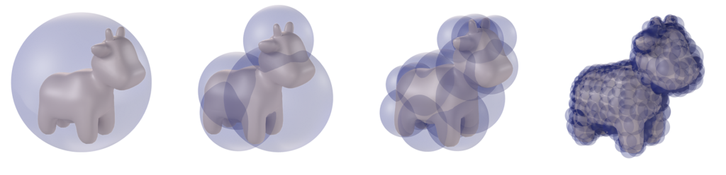
Figure 3: Wrapped BD-Tree for Spot at increasing recursion levels.

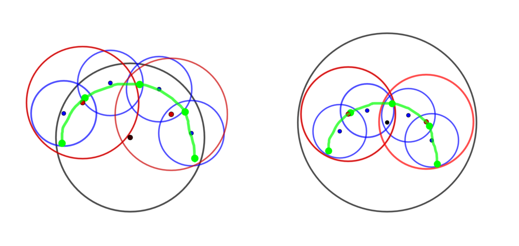
Now that we can compute the minimum bounding spheres for any set of points, we are ready to construct a hierarchical sphere tree on the undeformed model, after which it can be updated following deformation. First we note that the BD-Tree is a wrapped hierarchy, wherein the bounding spheres tightly enclose the underlying geometry but any bounding sphere at one level need not contain its child spheres. This is different from a layered hierarchy in which spheres must enclose their child spheres, but can fit the underlying geometry more loosely (see Figure 4).

Illustration of wrapped vs. layered BD-Trees — Figure 4: An illustration—re-created from [2] of the wrapped hierarchy (left) and layered hierarchy (right). The underlying geometry is shown in green with five vertices and four edges.

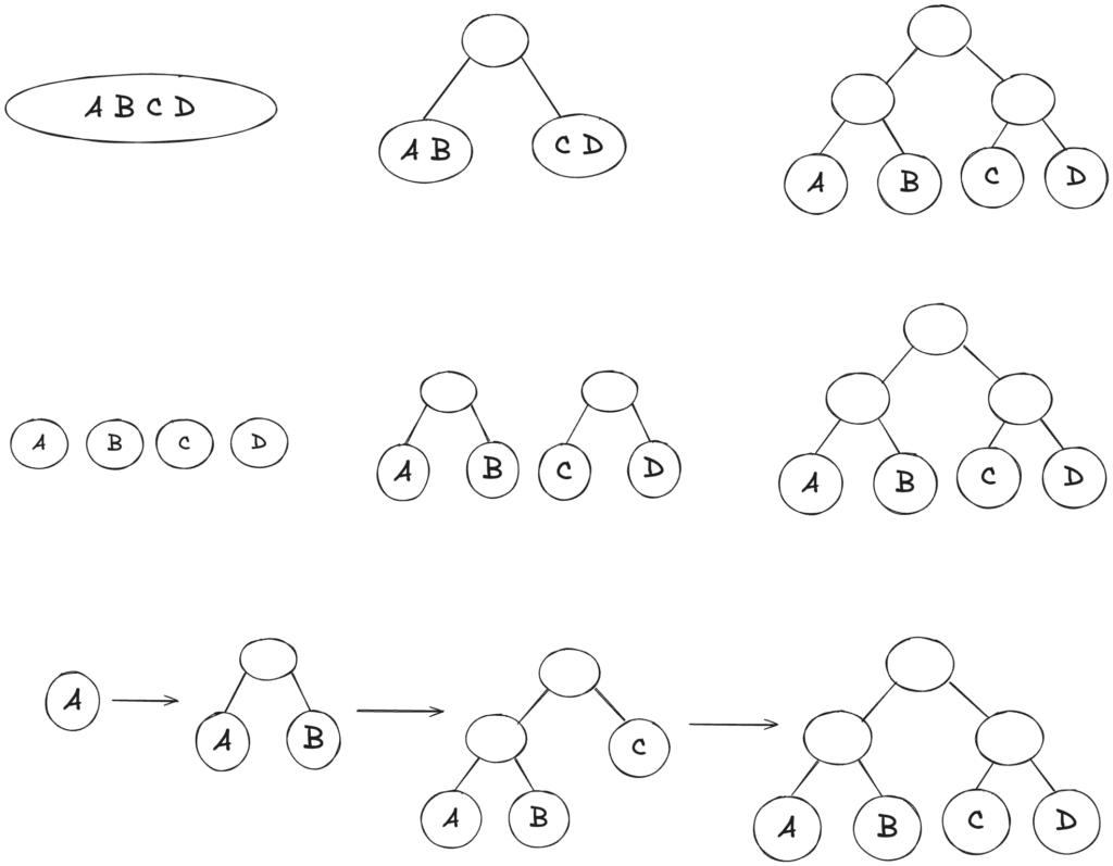
As shown in Figure 5, there are many possible approaches to building a binary tree. In our case, we use a simple top-down approach while partitioning the underlying geometry, i.e. we recursively split Spot at its median into two parts with respect to its local coordination axes, such that a leaf node (the lowest level) contains only one triangle.

Figure 5: Hierarchical binary tree construction with four objects using a top-down (top), bottom-up (middle) and insertion approach (bottom).

As the object deforms, how do we compute the new bounding spheres quickly and efficiently?

Let \(S\) denote a sphere in the hierarchical tree with center \(c\) and radius \(R\) containing the \(k\) points of the geometry \(\{p_{i}\}_{1 \leq i \leq k}\). After the deformation, the center of the sphere \(c\) is displaced by a weighted average of the contained points’ displacements \(u_{i}\) with weights \(\beta_i\) e.g. \(\beta_i := 1/k\) for \(1 \leq i \leq k\). So the new center can be expressed as

\(\displaystyle c’ = c + \sum_{i = 1}^{k} \beta_i u_i.\)

Using the displacement equation above, we can write \(u_i\) as the sum \(\sum_{j = 1}^{r} U_{ij} q_{j}\) and substitute this into the previous equation to obtain:

\(\displaystyle c’ = c + \sum_{j = 1}^{r} \left(\sum_{i = 1}^{k} \beta_i U_{ij}\right) q_j = c + \bar{U} \boldsymbol{q}.\)

To compute the new radius \(R’\), we make use of the triangle inequality

\(\displaystyle \max_{i = 1, \dots, k} || p’_{i} – c’_{i} ||_{2} \leq \max_{i = 1, \dots, k} \left(||p’_{i}||_{2} + ||c’_{i}||_{2} \right).\)

Expanding both \(p’_{i}\) and \(c’_{i}\) using their displacement equations and re-arranging the terms, we get that

\(\displaystyle R’ = R + \sum_{j = 1}^{r} \left( \max_{i = 1, \dots, k} ||U_{ij} – \bar{U}_{j}||_{2} \right) |q_j|.\)

Thus, we have an updated bounding sphere \(S’\) with its center \(c’\) and radius \(R’\) computed as functions of the reduced coordinates \(\boldsymbol{q}\).

Figure 6: Spot colliding with ground plane. The colors of the spheres change based on the ratio of \(R\) in the undeformed state to \(R’\) in the deformed state.

References

[1] Hang Si. TetGen, a Delaunay-based quality tetrahedral mesh generator. ACM Transactions on Mathematical Software, 41(2), 2015.

[2] Doug L. James and Dinesh K. Pai. BD-Tree: Output-Sensitive Collision Detection for Reduced Deformable Models. ACM Transactions on Graphics, 23(3), 2004.

[3] Emo Welzl. Smallest enclosing disks (balls and ellipsoids). New Results and New Trends in Computer Science, 555, 1991.

[4] Christer Ericson. Real-Time Collision Detection. CRC Press, Taylor & Francis Group. Chapter 4, p. 99-100. 2005.

Post author By hussein
Post date October 8, 2024
Tags bd-tree, collision-detection, Math, modal-analysis, sgi2024

Math

The Area of a Circle

_{Author: Ehsan Shams (Alexandria University, Egypt)}

“Since people have tried to prove obvious propositions,
they have discovered that many of them are false.”
Bertrand Russell

Archimedes proposed an elegant argument indicating that the area of a circle (disk) of radius \(r\) is \( \pi r^2 \). This argument has gained attention recently and is often presented as a “proof” of the formula. But is it truly a proof?

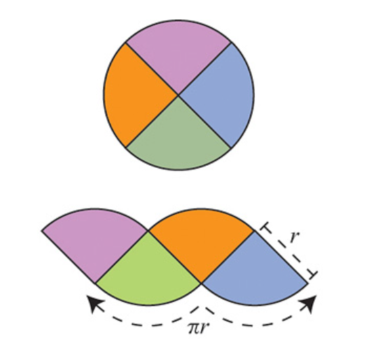
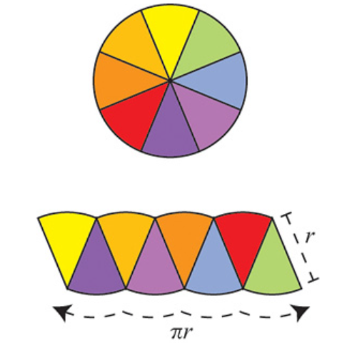
The argument is as follows: Divide the circle into \(2^n\) congruent wedges, and re-arrange them into a strip, for any \( n\) the total sum of the wedges (the area of the strip) is equal to the area of the circle. The top and bottom have arc length \( \pi r \). In the limit the strip becomes a rectangle, meaning as \( n \to \infty \), the wavy strip becomes a rectangle. This rectangle has area \( \pi r^2 \), so the area of the circle is also \( \pi r^2 \).

These images are taken from [1].

To consider this argument a proof, several things need to be shown:

The circle can be evenly divided into such wedges.
The number \( \pi \) is well-defined.
The notion of “area” of this specific subset of \( \mathbb{R}^2 \) -the circle – is well-defined, and it has this “subdivision” property used in the argument. This is not trivial at all; a whole field of mathematics called “Measure Theory” was founded in the early twentieth century to provide a formal framework for defining and understanding the concept of areas/volumes, their conditions for existence, their properties, and their generalizations in abstract spaces.
The limiting operations must be made precise.
The notion of area and arc length is preserved under the limiting operations of 4.

Archimedes’ elegant argument can be rigorised but, it will take some of work and a very long sheet of paper to do so.

Just to provide some insight into the difficulty of making satisfactory precise sense of seemingly obvious and simple-to-grasp geometric notions and intuitive operations which are sometimes taken for granted, let us briefly inspect each element from the above.

Defining \( \pi \):

In school, we were taught that the definition of \( \pi \) is the ratio of the circumference of a circle to its diameter. For this definition to be valid, it must be shown that the ratio is always the same for all circles, which is
not immediately obvious; in fact, this does not hold in Non-Euclidean geometry.

A tighter definition goes like this: the number \( \pi \) is the circumference of a circle of diameter 1. Yet, this still leaves some ambiguity because terms like “circumference,” “diameter,” and “circle” need clear definitions, so here is a more precise version: the number \( \pi \) is half the circumference of the circle \( \{ (x,y) | x^2 + y^2 =1 \} \subseteq \mathbb{R}^2 \). This definition is clearer, but it still assumes we understand what “circumference” means.

From calculus, we know that the circumference of a circle can be defined as a special case of arc length. Arc length itself is defined as the supremum of a set of sums, and in nice cases, it can be exactly computed using definite integrals. Despite this, it is not immediately clear that a circle has a finite circumference.

Another limiting ancient argument that is used to estimate and define the circumference of a circle and hence calculating terms of \( \pi \) to some desired accuracy since Archimedes was by using inscribed and circumscribed regular polygons. But still, making a precise sense of the circumference of a circle, and hence the number \( \pi \), is a quite subtle matter.

The Limiting Operation:

In Archimedes’ argument, the limiting operation can be formalized by regarding the bottom of the wavy strip (curve) as the graph of a function \(f_n \), and the limiting curve as the graph of a constant function \(f\). Then \( f_n \to f \) uniformly.

The Notion of Area:

The whole of Euclidean Geometry deals with the notions of “areas” and “volumes” for arbitrary objects in \( \mathbb{R}^2 \) and \( \mathbb{R}^3 \) as if they are inherently defined for such objects and merely need to be calculated. The calculation was done by simply cutting the object into finite simple parts and then rearranging them by performing some rigid motion like rotation or translation and then reassembling those parts to form a simpler body which we already know how to compute. This type of Geometry relies on three hidden assumptions:

Every object has a well-defined area or volume.
The area or volume of the whole is equal to the sum of the areas or volumes of its parts.
The area or volume is preserved under such re-arrangments.

This is not automatically true for arbitrary objects; for example consider the Banach-Tarski Paradox. Therefore, proving the existence of a well-defined notion of area for the specific subset describing the circle, and that it is preserved under the subdivision, rearrangement, and the limiting operation considered, is crucial for validating Archimedes’ argument as a full proof of the area formula. Measure Theory addresses these issues by providing a rigorous framework for defining and understanding areas and volumes. Thus, showing 1,3, 4, and the preservation of the area under the limiting operation requires some effort but is achievable through Measure Theory.

Arc Length under Uniform Limits:

The other part of number 5 is slightly tricky because the arc length is not generally preserved under uniform limits. To illustrate this, consider the staircase curve approximation of the diagonal of a unit square in \( \mathbb{R}^2 \). Even though as the step curves of the staircase get finer and they converge uniformly to the diagonal, their total arc length converges to 2, not to \( \sqrt{2} \). This example demonstrates that arc length, as a function, is not continuous with respect to uniform convergence. However, arc length is preserved under uniform limits if the derivatives of the functions converge uniformly as well. In such cases, uniform convergence of derivatives ensures that the arc length is also preserved in the limit. Is this provable in Archimedes argument? yes with some work.

Moral of the Story:

There is no “obvious” in mathematics. It is important to prove mathematical statements using strict logical arguments from agreed-upon axioms without hidden assumptions, no matter how “intuitively obvious” they seem to us.

“The kind of knowledge which is supported only by
observations and is not yet proved must be carefully
distinguished from the truth; it is gained by induction, as
we usually say. Yet we have seen cases in which mere
induction led to error. Therefore, we should take great
care not to accept as true such properties of the numbers
which we have discovered by observation and which are
supported by induction alone. Indeed, we should use such
a discovery as an opportunity to investigate more exactly
the properties discovered and to prove or disprove them;
in both cases we may learn something useful.”
–L. Euler

“Being a mathematician means that you don’t take ‘obvious’
things for granted but try to reason. Very often you will be
surprised that the most obvious answer is actually wrong.”
–Evgeny Evgenievich

Bibliography

Strogatz, S. (1270414824). Take It to the Limit. Opinionator. https://archive.nytimes.com/opinionator.blogs.nytimes.com/2010/04/04/take-it-to-the-limit/
Tao, T. (2011). An introduction to measure theory. Graduate Studies in Mathematics. https://doi.org/10.1090/gsm/126
Pogorelov, A. (1987). Geometry. MIR Publishers.
Blackadar, B. (2020). Real Analysis Notes

Post author By ehsan.ali
Post date August 17, 2024
Tags Math

Math Research

Spline Construction with Closed-form Arc-Length Solution: A Guided Tour

Post author By ehsan.ali
Post date August 8, 2024
No Comments on Spline Construction with Closed-form Arc-Length Solution: A Guided Tour

^{Author: Ehsan Shams (Alexandria Univerity, Egypt)
Project Mentor: Sofia Di Toro Wyetzner (Stanford University, USA)
Volunteer Teaching Assistant: Shanthika Naik (CVIT, IIIT Hyderabad, India)}

In my first SGI research week, I went on a fascinating exploratory journey into the world of splines under the guidance of Sofia Wyetzner, and gained an insight into how challenging yet intriguing their construction can be especially under tight constriants such as the requirement for a closed-form expression for their arc-length. This specific construction was the central focus of our inquiry, and the main drive for our exploration.

Splines are important mathematical tools for they are used in various branches of mathematics, including approximation theory, numerical analysis, and statistics, and they find applications in several areas such as Geometry Processing (GP). Loosely speaking, such objects can be understood as mappings that take a set of discrete data points and produce a smooth curve that either interpolates or approximates these points. Thus, it becomes natural immediately to see that they are of great importance in GP since, in the most general sense, GP is a field that is mainly concerned with transforming geometric data¹ from one form to another. For example, splines like Bézier and B-spline curves are foundational tools for curve representation in computer graphics and geometric design (Yu, 2024).

Having access to arc lengths for splines in GP is essential for many tasks, including path planning, robot modeling, and animation, where accurate and realistic modeling of curve lengths is critically important. For application-driven purposes, having a closed formula for arc-length computation is highly desirable. However, constructing splines with this arc-length property that can interpolate \( k \) arbitrary data points reasonably well is indeed a challenging task.

Our mentor Sofia, and Shanthika guided us through an exploration of a central question in spline formulation research, as well as several related tangential questions:

Our central question was:

Given \( k \) points, can we construct a spline that interpolates these points and outputs the intermediate arc-lengths of the generated, curve, with some continuity at control points?

And the tangential ones were:

1. Can we achieve \( G^1 \) / \( C^1\) / \( G^2 \) / \(C^2\) continuity at these points with our spline?
2. Given \(k\) points and a total arc-length, can we interpolate these points with the given arc-length in \( \mathbb{R}^2 \)?

In this article, I will share some of the insights I gained from my first week-long research journey, along with potential future directions I would like to pursue.

Understanding Splines and their Arc-length

What are Splines?

A spline is a mapping \( S: [a,b] \subset \mathbb{R} \to \mathbb{R}^n \) defined as:

\( S(t) = \begin{cases} s_1(t) & \text{for } t \in [t_0, t_1] \\ s_2(t) & \text{for } t \in [t_1, t_2] \\ \vdots \\ s_n(t) & \text{for } t \in [t_{n-1}, t_n] \end{cases} \)

where \( a = t_0 < t_1 < \cdots < t_n = b \), and \( s_i: [t_i, t_{i+1}] \to \mathbb{R}^n \) are defined such that, \(S(t)\) ensures \( C^k \) continuity at each internal point \( t_j \), meaning:

\( s_{i-1}^{(m)}(t_j) = s_i^{(m)}(t_j) \) for \( m = 0,1 \dots, k \)

where \( s_{i-1}^{(m)} \) and \( s_i^{(m)} \) are the \( m \)-th derivatives of \( s_{i-1}(t) \) and \( s_i(t) \) respectively.

In other words, a spline is a mathematical construct used to create a smooth curve \( S(t) \) by connecting a sequence of simpler piecewise segments \( s_i(t) \) in a continuous manner. These segments \( s_i(t) \) for \( i = 1, 2, \ldots, n \) are defined on subintervals \( [t_i, t_{i+1}] \) of the parameter domain, and are carefully joined end-to-end. The transitions at the junctions \( \{ t_i \}_{i=1}^{n-1} \) (also known as control points) maintain a desired level of smoothness, typically defined by the continuity of derivatives up to order \( k \) on \( \{s_i(t)\}_{i=1}^n \).

One way to categorize splines is based on the types of functions \(s_i\) they incorporate. For instance, some splines utilize polynomial functions such as Bézier splines and B-splines, while others may employ trigonometric functions such as Fourier splines or hyperbolic functions. However, the most commonly used splines in practice are those based on polynomial functions, which define one or more segments. Polynomial splines are particularly valuable in various applications because of their computational simplicity and flexibility in modeling curves.

Arc Length Calculation

Intuitively, the notion of arc-length of a curve² can be understood as the numerical measurement of the total distance traveled along the curve from one endpoint to another. This concept is fundamental in both calculus and geometry because it provides a way to quantify the length of some curves, which may not be a straight line. To calculate the arc length of smooth curves, we use integral calculus. Specifically, we apply a definite integral formula – (presented in the following theorem) but, let us first define the concept formally.

Definition. Let \( \gamma : [a, b] \to \mathbb{R}^n \) be a parametrized curve, and \( P = \{ a = t_0, t_1, \dots, t_n = b \} \) a partition of \( [a, b] \). The polygonal approximate³ length of \( \gamma \) from \(P\) is given by the sum of the Euclidean distances between the points \( \gamma(t_i)\) for \( i = 0, 1, \dots, n \):

\(L_P(\gamma) = \sum_{i=0}^{n} |\gamma(t_{i+1}) – \gamma(t_i)|\)

where \( | \cdot | \) denotes the Euclidean norm in \( \mathbb{R}^n \). This polygonal approximation becomes a better estimate of the actual length of the curve as the partition \( P\) becomes finer (i.e., as the maximum distance between successive \( t_i \) tends to zero). The actual length of the curve can be defined as:

\( L(\gamma) = \sup_P L_P(\gamma) \)

If the curve \( \gamma \) is sufficiently smooth, the actual length of the curve can be computed using definite integration as shown in the following theorem.

Arc Length Theorem. Let \( \gamma : [a, b] \to \mathbb{R}^n \) be a \( C^1 \) curve. The arc length \( L(\gamma) \) of \(\gamma\) is given by:

\( L(\gamma) = \int_a^b |\gamma'(t)| \, dt \)

where \(\gamma'(t) \) is the derivative of \(\gamma\) with respect to \(t\).

The challenge

As mentioned earlier, in the context of spline construction for GP tasks, ideally one is interested in constructing splines that have closed-form solutions for their arc length (a formula for computing their arc-length). However, curves with this property for their arc-length are relatively rare because the arc length integral often leads to elliptic integrals⁴ or other forms that do not have elementary antiderivatives. However, there are some curves for which the arc length can be computed exactly using a closed formula. Here are some examples: Straight lines, circles, and parabolas under certain conditions have closed-form solutions for arc length.

Steps to tackle the central question …

Circular Splines: A Starting Point.

In day one, our mentor Sofia went with us through a paper titled “A Class of \(C^2 \) Interpolating Splines” (Yuksel, 2020). In this work, the author introduces a novel class of non-polynomial parametric splines to interpolate given \( k \) control points. Two components define their class construction: interpolating functions and blending functions (defined later). Each interpolating function \(F_j \in \{F_i \}_{i=1}^n\) defines three consecutive control points, and the blending functions \( \{ B_i \}_{i=1}^m \) combines each two consecutive interpolating functions, forming a smooth curve between two control points. The blending functions are chosen so that \( C^2 \)-continuity everywhere is ensured independent of the choice of the interpolating functions. They use trignometric blending functions.

This type of formulation was constructed to attain some highly desirable properties in the resulting interpolating spline not previously demonstrated by other spline classes, including \( C^2 \) continuity everywhere, local support, and the ability to guarantee self-intersection-free curve segments regardless of the placement of control points and form perfect circular arcs. This paper served as a good starting point in light of the central question under consideration because among the interpolating functions they introduce in their paper are circular curves which have closed formulas for arc-length computation. In addition, it gives insight into the spline formulation practice. However, circular interpolating functions are not without their limitations; their constant curvature makes them difficult to reasonably interpolate arbitrary data, and they look bizarre sometimes.

Interesting note: The earliest documented reference – to the best of my knowledge – discussing the connection of two interpolating curves with a smooth curve dates back to Macqueen’s research in 1936 (MacQueen, 1936) Macqueen’s paper, titled “On the Principal Join of Two Curves on a Surface,” explores the concept of linking two curves on a surface.

Here is a demo constructed by the author to visualize the resulting output spline from their class with different interpolating functions, and below is me playing with the different interpolating functions, and looking at how bizarre the circular interpolating function looks when you throw out data points in an amorphus way.

While playing with the demo, the Gnomus musical track by Modest Mussorgsky was playing in parallel in the back of my mind so I put there for you too. It is a hilarious coincidence that the orchestra goes mad when it is the circular spline’s turn to interpolate the control points, and it does so oddly and bizarrely than the other splines in question. It even goes beyond the boundary of the demo. Did you notice that? 🙂

By the end of the day, I was left with two key inquiries, and a starting point for investigating them:

How do we blend desirable interpolating functions to construct splines with the properties we want? Can we use a combination of circular and elliptical curves to achieve more flexible and accurate interpolation for a wider variety of data points while maintaining a closed form for their arc length? What other combinations could serve us well?
I thought to myself: I should re-visit my functional analysis course as a starting point to think about this in a clear way.

From day two to five, we followed a structured yet not restrictive approach, akin to “we are all going to a definite destination but at the same time, everyone could stop by to explore something that captured their attention along the way if they want to and share what intrigued them with others”. This approach was quite effective and engaging:

Implementing a User-Interactive: Our first task was to develop a simple user interface for visualizing existing spline formulations. My SGI project team and friends—Charuka Bandara, Brittney Fahnestock, Sachin Kishan, and I—worked on this in Python (for Catmull-Rom splines) and MATLAB (for Cubic and Quadratic splines). This tool allowed us to visualize how different splines behave and change shape whenever the control points change, also restored my love for coding as I have not coded in a while … you know nothing is more joyful than watching your code executing exactly what you want it to do, right?
Below is a UI for visualizing a Cubic Spline. Find the UI for the Quadratic Spline, and the Catmull-Rom here.

Interactive Cubic Spline

Exploring Blending Functions Method: As a natural progression towards our central inquiry, and a complementary task to reading Yuksel’s paper, we eventually found our way to exploring blending functions—a topic I had been eagerly anticipating.

Here, I decided to pause and explore more about the blending function method in spline formulation.

The blending function method, is a method that provides a way to construct a spline \( S(t) \) as a linear combination of a set of control points \( \{p_i(t)\}_{i=1}^n \) and basis functions (blending functions) \( \{B_i(t)\}_{i=1}^n \) in the following manner:

\( S(t) = \sum_{i=1}^n p_i B_i(t)\) (*)

where:
\( t \): is the parameter defined over the interval of interest \( [a,b] \)

These blending functions \(B_i(t)\) typically exhibit certain properties that govern, for example, the smoothness, continuity, shape, and preservation of key characteristics that we desire in the resulting interpolating splines. Thus, by carefully selecting and designing those blending functions, it is possible to tailor the behaviour of spline interpolation to meet the specific requirements and achieve desired outcomes.

Below are some of the properties of important blending functions:

Partition of Unity: \( \sum_{i=1}^n B_i(t) =1, \forall t \in [a,b] \), also called coordinate system independent. This property is important because it provides a convex combination of the control points in question, and this is something you need to ensure that the curve does not change if the coordinate changes, one way to visualize this is by imagining that the control points in questions are beads sitting in an amorphous manner on a sheet of paper and the interpolating curve as a thread going through them, and you move the sheet of paper around, what we need is that the thread that goes through these beads does not move around as well, and this is what this property means. Notice that if you pick an arbitrary set of blending functions, this property is not immediately actualized, and the curve would change.
Local Support: Each blending function \( B_i(t) \neq 0 \forall t \in I and i=1,2, … , n \) where \(I \subset [a,b] \) is the interval of interest and vanishes everywhere else on the domain. This property is important because it ensures computational efficiency. With this property actualized in one’s blending functions, one does not have to worry about consequences on their interpolating curve if they are to modify one control point .. for it will only affect a local region in the curve, and not the entire curve.
Non-negativity: Blending functions are often non-negative over the domain of definition \( [a,b] \). This property is called convex hull. It is important for maintaining stability and predictability of the interpolating spline. It prevents the curve from oscillating wildly or provides unfaithful representation of the data point in question.
Smoothness: Blending functions dictate the overall smoothness of the resulting spline since the space of \( C^k (\mathcal{K})\) ( \(k\)-times continously differentiable functions defined on a closed and compact set \(\mathcal{K}\) is a vector space over \(\mathbb{R}\) or \(\mathbb{C}\).
Symmetry: Blending functions that are symmetric about the central control point, do not change if the points are ordered in reverse. In this context, symmetry is assured, if and only if, \( \sum_{i=1}^n B_i(t) p_i = \sum_{i=1}^n B_i ((a+b)-t) p_{n-i} \) this holds if \(B_i(t) = B_{n-i}((a+b)-t) \). For instance, Timmer’s parametric cubic, and Ball’s cubic – (a variant of cubic Bézier) – curve obey this property.

In principle, there can be as many properties imposed on the blending functions depending on the desired aspects one wants in their interpolating spline \( S(t) \).

Remark. The spline formulation (*) describes the weighted sum of the given control points \( \{p_i\}_{i=1}^n\). In other words, each control point is influencing the curve by pulling it in its direction, and the associated blending function is what determines the strength of this influence and pull. Sometimes, one does not need to use blending functions in trivial cases.

Brain-storming for new spline formulation: Finally, we were prepared for our main task. We brainstormed new spline formulations, in doing so, we first looked at different interpolating curves such as catenaries, parabolas, circles for interpolation and arc-length calculation, explored \(C^1\) and \( C^2 \) continuity at control points, did the math on papers, which something I miss nowadays, for the 3-point, and then laid down the foundation for the \(k\)-point interpolation problem. I worked with the parabolas because I love them.

In parallel, I looked a bit into tangential question two … it is an interesting question:

Given \(k\) points and a total arc-length \(L\), can we interpolate these points with the given arc-length in \(\mathbb{R}^2 \)?

From the polynomial interpolation theorem, we know that for any set of \( k \) distinct points \((x_1, y_1), (x_2, y_2), \ldots, (x_k, y_k) \in \mathbb{R}^2 \), there exists a polynomial \( P(x) \) of degree \( k-1 \) such that: \(P(x_i) = y_i \text{ for } i = 1, 2, \ldots, k.\). Such a polynomial is smooth and differentiable (i.e., it is a \( C^\infty \) function) over \( \mathbb{R} \) thus rectifiable so it possesses a well-defined finite arc-length over any closed interval.

Now, let us parameterize the polynomial \( P(x) \) as a parametric curve \( \mathbf{r}(t) = (t, P(t)) \), where \( t \) ranges over some interval \([a, b] \subset \mathbb{R}\).

Now let us compute its arc-length,

The arc-length \( S \) of the curve \( \mathbf{r}(t) = (t, P(t)) \) from \( t = a \) to \( t = b \) is given by:

\( S = \int_a^b \sqrt{1 + \left(\frac{dP(t)}{dt}\right)^2} \, dt. \)

To achieve the desired total arc-length \( L \), we rescale the parameter \( t \). Define a new parameter \( \tau \) as: \( \tau = \alpha t. \)

Now, the new arc-length ( S’ ) in terms of \( \tau \) is:

\( S’ = \int_{\alpha a}^{\alpha b} \sqrt{1 + \left(\frac{dP(\tau / \alpha)}{d(\tau / \alpha)}\right)^2} \frac{d(\tau / \alpha)}{d\tau} \, d\tau.\)

Since \( \frac{d(\tau / \alpha)}{d\tau} = \frac{1}{\alpha} \), this simplifies to:

\( S’ = \int_{\alpha a}^{\alpha b} \sqrt{1 + \left(\frac{dP(\tau / \alpha)}{d(\tau / \alpha)}\right)^2} \frac{1}{\alpha} \, d\tau.\)

\(S’ = \frac{1}{\alpha} \int_{\alpha a}^{\alpha b} \sqrt{1 + \left(\frac{dP(\tau / \alpha)}{d(\tau / \alpha)}\right)^2} \, d\tau.\)

\(S’ = \frac{S}{\alpha}.\). To ensure \( S’ = L \), choose \( \alpha = \frac{S}{L} \).

Thereby, by appropriately scaling the parameter \( t \), we can adjust the arc-length to match \( L \). Thus, there exists a curve \( C \) that interpolates the \( k \geq 2 \) given points and has the total arc-length \( L \) in \( \mathbb{R}^2 \).

Now, what about implementation? how could we implement an algorithm to execute this task?

It is recommended to visualize your way through an algorithm on a paper first, then formalize to words and symbols, make sure there are no semantic errors in the formalization then code then debug. You know debugging is one of the most intellectually stimulating exercises, and exhausting ones. I am a MATLAB person so here is a MATLAB function you could use to achieve this task ..

function [curveX, curveY] = curveFunction(points, totalArcLength)
    % Input: 
    % points - Nx2 matrix where each row is a point [x, y]
    % totalArcLength - desired total arc length of the curve
    
    % Output:
    % curveX, curveY - vectors of x and y coordinates of the curve
    
    % Number of points
    n = size(points, 1);
    
    % Calculate distances between consecutive points
    distances = sqrt(sum(diff(points).^2, 2));
    
    % Calculate cumulative arc length
    cumulativeArcLength = [0; cumsum(distances)];
    
    % Normalize cumulative arc length to range from 0 to 1
    normalizedArcLength = cumulativeArcLength / cumulativeArcLength(end);
    
    % Desired number of points on the curve
    numCurvePoints = 100; % Change as needed
    
    % Interpolated arc length for the curve
    curveArcLength = linspace(0, 1, numCurvePoints);
    
    % Interpolated x and y coordinates
    curveX = interp1(normalizedArcLength, points(:, 1), curveArcLength, 'spline');
    curveY = interp1(normalizedArcLength, points(:, 2), curveArcLength, 'spline');
    
    % Scale the curve to the desired total arc length
    scale = totalArcLength / cumulativeArcLength(end);
    curveX = curveX*scale;
    curveY = curveY*scale;

    %plot(curveX, curveY);

 % Plot the curve
    figure;
    plot(curveX, curveY);
    hold on;
    title('Curve Interpolation using Arc-Length and Points');
    xlabel('X');
    ylabel('Y');
    grid on;
    hold off;
end

Key Takeaways, and Possible Research Directions:

Key Takeaway:

Splines are important!
Constructing them is nontrivial especially under multiple conflicting constraints, as it significantly narrows the feasible search space of potential representative functions.
Progress in abstract mathematics makes the lives of computational engineers and professionals in applied numerical fields easier, as it provides them with greater spaces for creativity and discoveries of new computational tools.

Possible Future Research Directions:

“I will approach this question as one approaches a

hippopotamus: stealthily and from the side.”

– R. Mahony

I borrowed this quote from Prof. Justin Solomon’s Ph.D. thesis. I read parts of it this morning and found that the quote perfectly captures my perspective on tackling the main question of this project. In this context, the “side” approach would involve exploring the question through the lens of functional analysis. 🙂

Acknowledgments. I would like to express my sincere gratitude to our project mentor Sofia Di Toro Wyetzner and Teaching Assistant Shanthika Naik for their continuous support, guidance, and insights to me and my project fellows during this interesting research journey, which prepared me well for my second project on “Differentiable Representations for 2D Curve Networks”. Moreover, I would like to thank my team fellows Charuka Bandara, Brittney Fahnestock, and Sachin Kishan for sharing interesting papers which I am planning to read after SGI!