Fellows: Sachin Kishan and Diany Pressato
Teaching Assistant: Supriya Gadi Patil
Mentor: Ahmed Mahmoud
Introduction
RXMesh is a framework for processing triangle mesh on the GPU. It allows developers to easily use the GPU’s massive parallelism to perform common geometry processing tasks on triangle mesh. For a preliminary introduction to RXMesh, check out this tutorial blog here.
Our task was to use RXMesh to implement some classic algorithms in geometry processing. This blog details one of the algorithms we implemented: Spectral Conformal Parameterization (SCP).
This blog will discuss the algorithm in terms of its basic concepts, the steps of the algorithm, the implementation using RXMesh, and our results.
Our entire implementation of SCP application in RXMesh can be found here.
Spectral Conformal Parameterization
Parameterization refers to the mapping of a triangle surface mesh in \(R^{3}\) space to a planar \(R^{2}\) space. This mapping can then be subsequently used in different application such as texture mapping, where we map the values from some other \(R^{2}\) space (e.g., image) to the surface of the mesh. In this case, we map color values to the mesh surface.
Often when we perform mesh parameterization, there is a possibility to change some properties of the geometric elements of the mesh, such as the size, shape, or angle between edges. It is desired to preserve these properties since we usually want to create a direct mapping of our intended values (e.g., texture color) to be in the “correct” positions on the mesh. What is correct is usually up to artistic opinion, and thus a mapping that preserves these properties is desirable. A mapping that conserves angles (and thus shape) is called a conformal mapping.
Mullen et al. (2008) provides a method to perform conformal parameterization of an open surface mesh by modelling the problem as a generalized Eigenvalue problem. Using an initial guess, we can perform multiple iterations of a general eigen vector solving method (i.e., the power method [2] ) to determine the largest eigen vector. This eigen vector, in our case, is the parameterized coordinates of the given mesh, giving us our desired output.
The algorithm for the power method is as follows:
Given \((A-\lambda B)x=0 \)
We want to find \(x\).
Given an initial guess of eigen-vector \(x_{0}\)
For some number of iterations, on iteration k
- \(B y_{k+1} = A x_{k}\)
- \(x_{k+1}= \frac{y_{k+1}}{\left| y_{k+1} \right|} \)
where \(x\) is the desired eigenvector solution.
Implementation
We applied the power method to our application in the following way, based on the formulation given by Mullen et al. (2008) in equation 7:
\([B-\frac{1}{V_{b}}e_{b}e_{b}^{t}]u=\mu L_{c}u \)
To find the eigenvector \(u\), we can the power method since the problem is in the form \(B y_{k+1} = A x_{k}\). This can be done in the following way:
\(T2=dot(eb,u) \)
\(T1=Bu – T2 * eb \)
\(L_{c}u=T1 \)
\(u=u/normalise (u) \)
Where \(u\) is the parameterized coordinates. \(T1\) and \(T2\) are temporary variables to store certain scalar or vector values. Other variables are explained by Mullen et al. (2008). This loop can be implemented like this using RXMesh:
for (int i = 0; i < iterations; i++)
{
    cuComplex T2 = eb.dot(uv_mat);
    rx.for_each_vertex(rxmesh::DEVICE,
                       [eb, T2, T1, uv_mat, B] __device__(
                       const rxmesh::VertexHandle vh) mutable
                       {
                           T1(vh, 0) =
                       cuCsubf(cuCmulf(B(vh, vh), uv_mat(vh, 0)),
                       cuCmulf(eb(vh, 0), T2));
                       });

    Lc.solve(T1, uv_mat);
    float norm = uv_mat.norm2();
    uv_mat.multiply(1.0f / norm);
    if (std::abs(prv_norm - norm) < 0.0001)//convergence check
    {
        break;
    }
    prv_norm = norm;
}
\(T1\) is a vector whose values are per-vertex, which is why we perform a per vertex computation. \(T2\) is a scalar in which we store the value of the dot product dot(eb,uv).
Since our system matrix \(L_{c}\) has dimensions 2V x 2V, we use complex representations of value entries in the vectors and matrices we use. So, for example, our \(L_{c}\) matrix now has dimensions V x V where each entry is a complex number (with a real and complex part).
This means subsequent computations must use CUDA functions that operate on complex numbers (e.g., cuCsubf which subtracts complex numbers).
All initial pre-computations only allocate to the real part of the entry, except for the calculation of the area term \(A\) where we calculate \(L_{c}=L_{D}-A\) . For the area term, we assign values to the complex part of the area term. \(L_{D}\) represents the standard Laplace-Beltrami operator, which we calculate using the cotangent edge weights and assign to the real part.
After we obtain the eigenvector \(u\) in complex form, we can convert it to a standard V x 2 matrix form and use that for further processing (such as rendering).
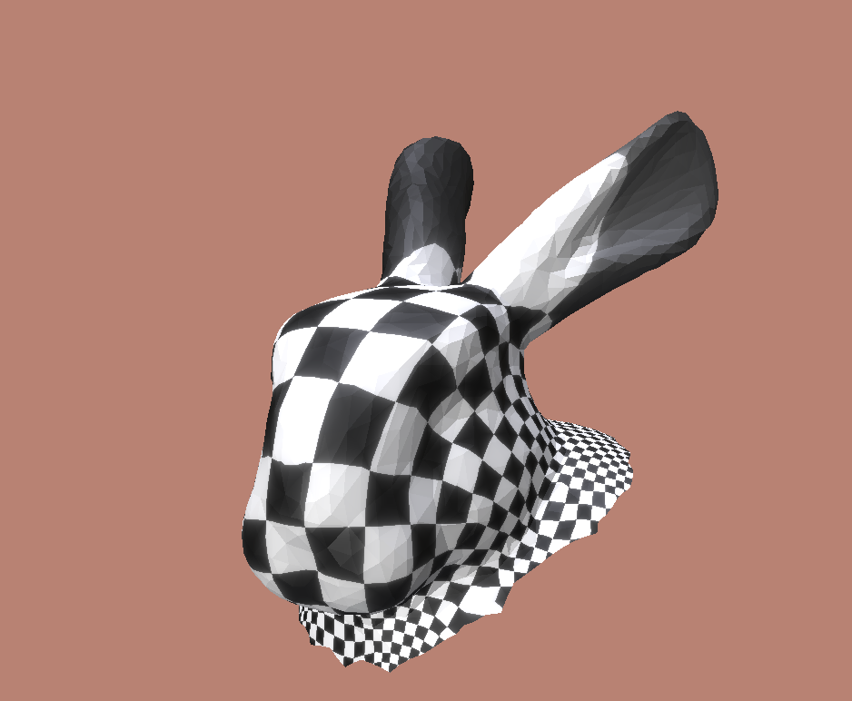
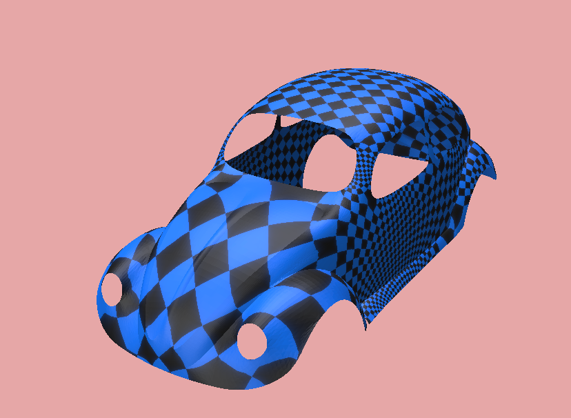
Results
Using the SCP implementation, we can now apply texturing to our open meshes as shown in the examples below.
References
[1] Mullen, P., Tong, Y., Alliez, P., & Desbrun, M. (2008). Spectral Conformal Parameterization. Computer Graphics Forum, 27(5), 1487–1494. https://doi.org/10.1111/j.1467-8659.2008.01289.x
[2] Kozłowski, W. (1992). The power method for the generalized eigenvalue problem. Roczniki Polskiego Towarzystwa Matematycznego. Seria 3, Matematyka Stosowana/Matematyka Stosowana/Mathematica Applicanda, 21(35). https://doi.org/10.14708/ma.v21i35.1790
This blog was written by Sachin Kishan and Diany Pressato during the SGI 2024 Fellowship as one of the outcomes of a two-week project under the mentorship of Ahmed Mahmoud and the support of Supriya Gadi Patil as a teaching assistant.