By Joana Portmann, Tal Rastopchin, and Sahra Yusuf.
Mentored by Professor Keenan Crane.
Intrinsic parameterization
During these last two weeks, we explored intrinsic encoding of triangle meshes. As an introduction to this new topic, we wrote a very simple algorithm that lays out a triangle mesh flat. We then improved this algorithm via line search over a week. In connection with this, we looked into terms like ‘angle defects,’ ‘cotangent weights,’ and the ‘cotangent Laplacian’ in preparation for more current research during the week.
From intrinsic to extrinsic parameterization
To get a short introduction into intrinsic parameterization and its applications, I quote some sentences from Keenan’s course. If you’re interested in the subject I can recommend the course notes “Geometry Processing with Intrinsic Triangulations.” “As triangle meshes are a basic representation for 3D geometry, playing the same central role as pixel arrays in image processing, even seemingly small shifts in the way we think about triangle meshes can have major consequences for a wide variety of applications. Instead of thinking about a triangle as a collection of vertex positions in \(\mathbb{R}^n\) from the intrinsic perspective, it’s a collection of edge lengths associated with edges.”
Many properties of a surface such as the shortest path do only depend on local measurements such as angles and distances along the surfaces and do not depend on how the surface is embedded in space (e.g. vertex positions in \(\mathbb{R}^n\)), so an intrinsic representation of the mesh works fine. Intrinsic triangulations bring several deep ideas from topology and differential geometry into a discrete, computational setting. And the framework of intrinsic triangulations is particularly useful for improving the robustness of existing algorithms.
Laying out edge lengths in the plane
Our first task was to implement a simple algorithm that uses intrinsic edge lengths and a breadth-first search to flatten a triangle mesh onto the plane. The key idea driving this algorithm is that given just a triangle’s edge lengths we can use the law of cosines to compute its internal angles. Given a triangle in the plane we can use the internal angles to flatten out its neighbors into the plane. We will later use these angles to modify the edge lengths so that we “better” flatten the model. The algorithm works by choosing some root triangle and then performing a breadth-first traversal to flatten each of the adjacent triangles into the plane until we have visited every triangle in the mesh.
Breadth-first search pseudocode
Some initial geometry central pseudocode for this breadth first search looks something like
// Pick and flatten some starting triangle
Face rootTriangle = mesh->face(0);

// Calculate the root triangle’s flattened vertex positions
calculateFlatVertices(rootTriangle);

// Initialize a map encoding visited faces
FaceData<bool> isVisited(*mesh, false);

// Initialize a queue for the BFS
std::queue<Face> visited;

// Mark the root triangle as visited and pop it into the queue
isVisited[rootTriangle] = true;
visited.push(rootTriangle);

// While our queue is not empty
while(!visited.empty())
{
    // Pop the current Face off the front of the queue
    Face currentFace = visited.front();
    visited.pop();

    // Visit the adjacent faces
    For (Face adjFace : currentFace.adjacentFaces()) {
        // If we have not already visited the face
        if (!visited[adjFace]
            // Calculate the triangle’s flattened vertex positions
            calculateFlatVertices(adjFace);
            // And push it onto the queue
            visited.push(adjFace);
        }
    }
}
In order to make sure we lay down adjacent triangles with respect to the computed flattened plane coordinates of their parent triangle we need to know exactly how a child triangle connects to its parent triangle. Specifically, we need to know which edge is shared by the parent and child triangle and which point belongs to the child triangle but not the parent triangle. One way we could retrieve this information is by computing the set difference between the vertices belonging to the parent triangle and child triangle, all while carefully keeping track of vertex indices and edge orientation. This certainly works, however, it can be cumbersome to write a brute force combinatorial helper method for each unique mesh element traversal routine.
The halfedge mesh data structure
Professor Keenan Crane explained that a popular mesh data structure that allows a scientist to conveniently implement mesh traversal routines is that of the halfedge mesh. At its core a halfedge mesh encodes the connectivity information of a combinatorial surface by keeping track of a set of halfedges and the two connectivity functions known as twin and next. Here the set of halfedges are none other than the directed edges obtained from an oriented triangle mesh. The twin function takes a halfedge and brings it to its corresponding oppositely oriented twin halfedge. In this fashion, if we apply the twin function to some halfedge twice we get the same initial halfedge back. The next function takes a halfedge and brings it to the next halfedge in the current triangle. In this fashion if we take the next function and apply it to a halfedge belonging to a triangle three times, we get the same initial halfedge back.

Professor Keenan Crane has a well written introduction to the halfedge data structure in section 2.5 of his course notes on Discrete Differential Geometry.
It turns out that geometry central uses the halfedge mesh data structure and so we can rewrite the traversal of the adjacent faces loop to more easily retrieve our desired connectivity information. In the geometry central implementation, every mesh element (vertex, edge, face, etc.) contains a reference to a halfedge, and vice versa.
// Pop the current Face off the front of the queue
Face currentFace = visited.front();
visited.pop();

// Get the face’s halfedge
Halfedge currentHalfedge = currentFace.halfedge();

// Visit the adjacent faces
do
{
    // Get the current adjacent face
    Face adjFace = currentHalfedge.twin().face();
    if (!isVisited[adjFace])
    {
        // Retrieve our desired vertices
        Vertex a = currentHalfedge.vertex();
        Vertex b = currentHalfedge.next().vertex();
        Vertex c = currentHalfedge.twin().next().next().vertex();

        // Calculate the triangle’s flattened vertex positions
        calculateFlatVertices(a, b, c);
        // And push it onto the queue
        visited.push(adjFace);
    }
    // Iterate to the next halfedge
    currentHalfEdge = currentHalfEdge.next();
}
// Exit the loop when we reach our starting halfedge
while (currentHalfEdge != currentFace.halfedge());
Here’s a diagram illustrating the relationship between the currentHalfedge and vertices a, b, and c.
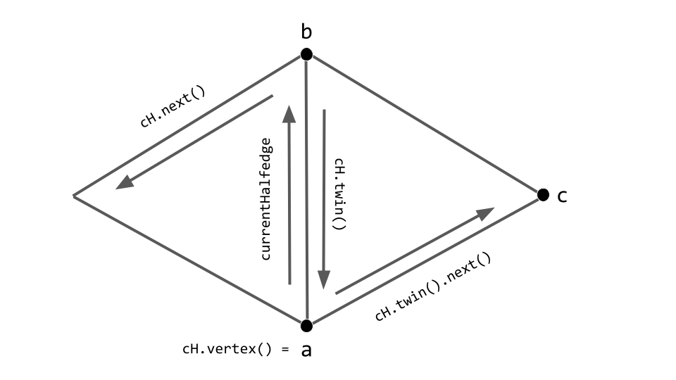
currentHalfedge and vertices a, b, and c. Note that cH abbreviates currentHalfedge.Segfaults, debugging, and ghost faces
This all looks great right? Now we need to determine the specifics of calculating the flat vertices? Well, not exactly. When we were running a version of this code in which we attempted to visualize the resulting breadth-first traversal we encountered several random segfaults. When Sahra ran a debugger (shout out to GDB and LLDB 🥰) we learned that the culprit was the isVisited[adjFace] function call on the line
if (!isVisited[adjFace])
We were very confused as to why we would be getting a segfault while trying to retrieve the value corresponding to the key adjFace contained in the map FaceData<bool> isVisited. Sahra inspected the contents of the adjFace object and observed that it had index 248 whereas the mesh we were testing the breadth-first search on only had 247 faces. Because C++ zero indexes its elements, this means we somehow retrieved a face with index out of range by 2! How could this have happened? How did we retrieve that face in the first place? Looking at the lines
// Get the current adjacent face
Face adjFace = currentHalfedge.twin().face();
we realized that we made an unsafe assumption about currentHalfedge. In particular, we assumed that it was not a boundary edge. What does the twin of a boundary halfedge that has no real twin look like? If the issue we were running to was that the currentHalfedge was a boundary halfedge, why didn’t we get a segfault on simply currentHalfedge.twin()? Doing some research, we found that the geometry central internals documentation explains that
“We can implicitly encode the
Geometry central internals documentationtwin()relationship by storing twinned halfedges adjacent to one another– that is, the twin of an even-numbered halfedge numberedheishe+1, and the twin of and odd-numbered halfedge ishe-1.”
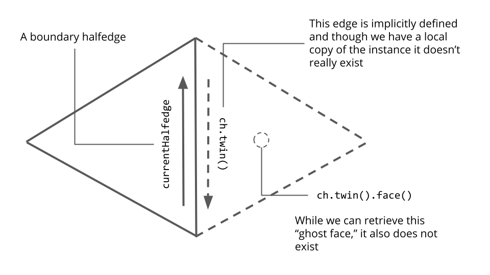
Aha! This explains exactly why currentHalfedge.twin() still works on a boundary halfedge; behind the scenes, it is just adding or subtracting one to the halfedge’s index. Where did the face index come from? We’re still unsure, but we realized that the face currentHalfedge.twin().face() only makes sense (and hence can only be used as a key for the visited map) when currentHalfedge is not a boundary halfedge. Here is a diagram of the “ghost face” that we think the line Face adjFace = currentHalfedge.twin().face() was producing.
Changing the map access line in the if statement to
if (!currentHalfedge.edge().isBoundary() && !isVisited[adjFace])
resolved the segfaults and produced a working breadth-first traversal.
Conformal parameterization
Here is a picture illustrating applying the flattening algorithm to a model of a cat head.
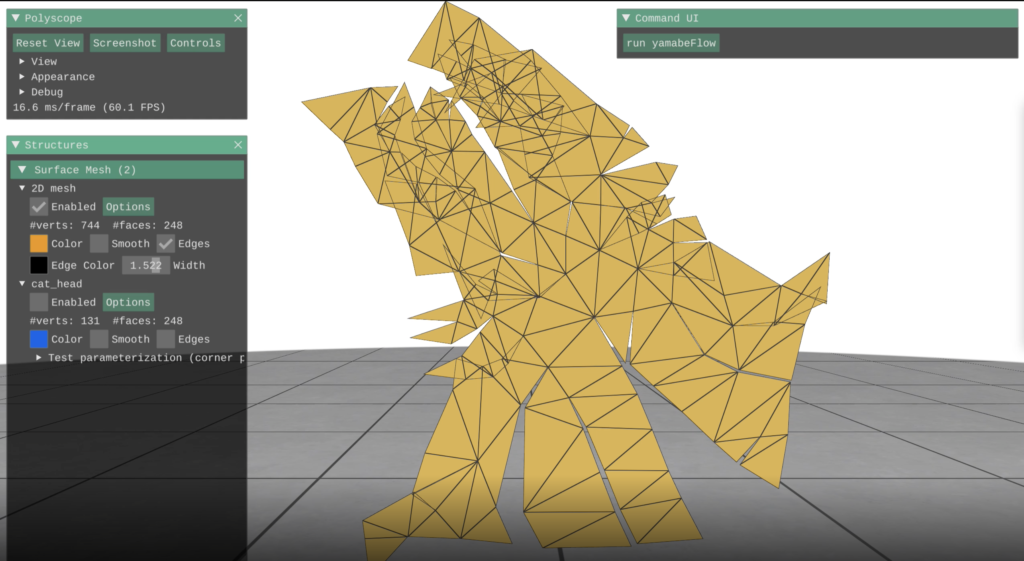
You can see that there are many cracks and this is because the model of the cat head is not flat—in particular, it has vertices with nonzero angle defect. A vertex angle defect for a given vertex is equal to the difference between \(2 \pi\) and the sum of the corner angles containing that vertex. This is a good measure of how flat a vertex is because for a perfectly flat vertex, all angles surrounding it will sum to \(2 \pi\).
After laying out the edges on the plane \(z=0\), we began the necessary steps to compute a conformal flattening (an angle-preserving parameterization). In order to complete this step, we needed to find a set of new edge lengths which would both be related to the original ones by a scale factor and minimize the angle defects,
\(l_{ij} := \sqrt{ \phi_i \phi_j} l_{ij}^0, \quad \forall ij \in E\),
where where \(l_{ij}\) is the new intrinsic edge length, \(\phi_i, \phi_j\) are the scale factors at vertices \(i, j\), and \(l_{ij}^0\) is the initial edge length.
Discrete Yamabe flow
At this stage, we have a clear goal: to optimize the scale factors in order to scale the edge lengths and minimize the angle defects across the mesh (i.e. fully flatten the mesh). From here, we use the discrete Yamabe flow to meet both of these requirements. Before implementing this algorithm, we began by substituting the scale factors with their logarithms
\(l_{ij} = e^{(u_i + u_j)/2} l_{ij}^0\),
where \(l_{ij}\) is the new intrinsic edge length, \(u_i, u_j\) are the scale factors at vertices \(i, j\), and \(l_{ij}^0\) is the initial edge length. This ensures the new intrinsic edge lengths are always positive and that the optimization is convex.
To implement the algorithm, we followed this procedure:
1. Calculate the initial edge lengths
2. While all angle defects are below a certain threshold epsilon:
- Compute the scaled edge lengths
- Compute the current angle defects based on the new interior angles based on the scaled edge lengths
- Update the scale factors using the step and the angle defects:
\(u_i \leftarrow u_i – h \Omega _i\),
where \(u_i\) is the scale factor of the \(i\)th vertex, \(h\) is the gradient descent step size, and \(\Omega_i\) is the intrinsic angle defect at the \(i\)th vertex.
After running this algorithm and displaying the result, we found that we were able to obtain a perfect conformal flattening of the input mesh (there were no cracks!). There was one issue, however: we needed to manually choose a step size that would work well for the chosen epsilon value. Our next step was to extend our current algorithm by implementing a backtracking line search which would change the step size based on the energy.
Results
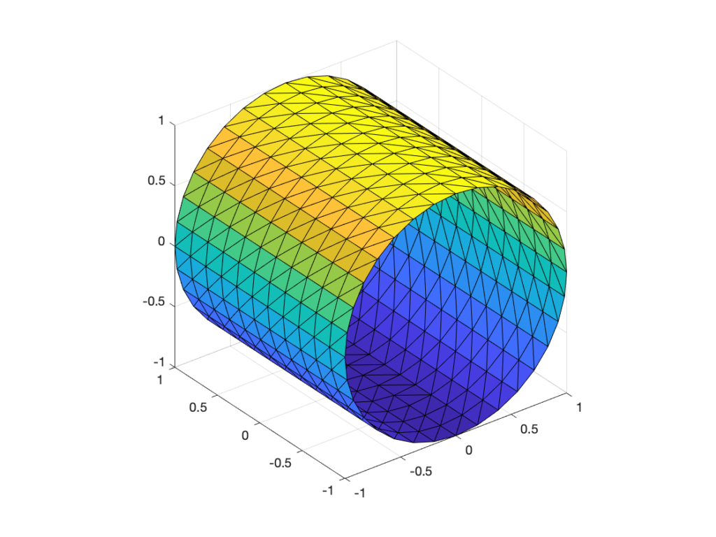
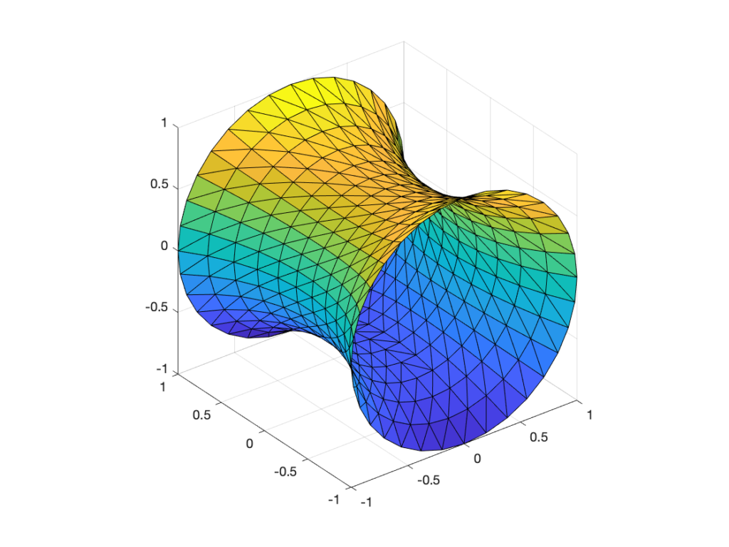
Here are two videos demonstrating the Yamabe flow algorithm. The first video illustrates how each iteration of the flow improves the flattened mesh and the second video illustrates how that translates into UV coordinates for texture mapping. We are really happy with how these turned out!
Line search
To implement this, we added a sub-loop to our existing Yamabe flow procedure which repeatedly test smaller step sizes until one is found which will decrease the energy, e.g., backtracking line search. A good resource on this topic is Stephen Boyd, Stephen P Boyd, and Lieven Vandenberghe. Convex optimization. Cambridge university press, 2004. After resolving a bug in which our step size would stall at very small values with no progress, we were successful in implementing this line search. Now, a large step size could be given without missing the minima.
Newton’s method
Next, we worked on using Newton’s method to improve the descent direction by changing the gradient to more easily reach the minimum. To complete this, we needed to calculate the Hessian — in this case, the Hessian of the discrete conformal energy was the cotan-Laplace matrix \(L\). This matrix had square dimensions (the number of rows and the number of columns was equal to the number of interior vertices) and has off-diagonal entries:
\(L_{ij} = -\frac{1}{2} (\cot \theta_k ^{ij} + \cot \theta _k ^{ji})\)
for each edge \(ij\), as well as diagonal entries
\(L_{ii} = – \sum _{ij} L_{ij}\)
for each edge \(ij\) incident to the \(i\)th vertex.
The newton’s descent algorithm is as follows:
- First, build the cotan-Laplace matrix L based on the above definitions
- Determine the descent direction \(\dot{u} \in \mathbb{R}^{|V_{\text{int}}|}\), by solving the system \(L \dot{u} = – \Omega\) with \(\Omega \in \mathbb{R}^{|V_{\text{int}}|}\).as the vector containing all of the angle defects at interior vertices.
- Run line search again, but with \(\dot{u}\) replacing \(– \Omega\) as the search direction.
This method yielded a completely flat mesh with no cracks. Newton’s method was also significantly faster: on one of our machines, Newton’s method took 3 ms to compute a crack-free parameterization for the cat head model while the original Yamabe flow implementation took 58 ms.