Categories
Demo SGI research projects

Self-similarity loss for shape descriptor learning in correspondence problems

By Faria Huq, Kinjal Parikh,  Lucas Valença

During the 4th week of SGI, we worked closely with Dr. Tal Shnitzer to develop an improved loss function for learning functional maps with robustness to symmetric ambiguity. Our project goal was to modify recent weakly-supervised works that generated deep functional maps to make them handle symmetric correspondences better.

Introduction:

  • Shape correspondence is a task that has various applications in geometry processing, computer graphics, and computer vision – quad mesh transfer, shape interpolation, and object recognition, to name a few. It entails computing a mapping between two objects in a geometric dataset. Several techniques for computing shape correspondence exist – functional maps is one of them. 
  • A functional map is a representation that can map between functions on two shapes’ using their eigenbases or features (or both). Formally, it is the solution to \(\mathrm{arg}\min_{C_{12}}\left\Vert C_{12}F_1-F_2\right\Vert^2\), where \(C_{12}\) is the functional map from shape \(1\) to shape \(2\) and  \(F_1\), \(F_2\) are corresponding functions projected onto the eigenbases of the two shapes, respectively.

Therefore, there is no direct mapping between vertices in a functional map. This concise representation facilitates manipulation and enables efficient inference.

Figure 1: The approach proposed by Sharma and Ovsjanikov may fail on symmetric regions. Notice the hands, which have not been matched correctly due to their symmetric structure.
  • Recently, unsupervised deep learning methods have been developed for learning functional maps. One of the main challenges in such shape correspondence tasks is learning a map that differentiates between shape regions that are similar (due to symmetry). We worked on tackling this challenge.

Background

  • We build upon the state-of-the-art work “Weakly Supervised Deep Functional Map for Shape Matching” by Sharma and Ovsjanikov, which learns shape descriptors from raw 3D data using a PointNet++ architecture. The network’s loss function is based on regularization terms that enforce bijectivity, orthogonality, and Laplacian commutativity.
  • This method is weakly supervised because the input shapes must be equally aligned, i.e., share the same 6DOF pose. This weak supervision is required because PointNet-like feature extractors cannot distinguish between left and right unless the shapes share the same pose.
  • To mitigate the same-pose requirement, we explored adding another component to the loss function Contextual Loss by Mechrez et al. Contextual Loss is high when the network learns a large number of similar features. Otherwise, it is low. This characteristic promotes the learning of global features and can, therefore, work on non-aligned data.

Work

  1. Model architecture overview: As stated above, our basic model architecture is similar to “Weakly Supervised Deep Functional Map for Shape Matching” by Sharma and Ovsjanikov. We use the basic PointNet++ architecture and pass its output through a \(4\)-layer ResNet model. We use the output from ResNet as shape features to compute the functional map. We randomly select \(4000\) vertices and pass them as input to our PointNet++ architecture.
  2. Data augmentation: We randomly rotated the shapes of the input dataset around the “up” axis (in our case, the \(y\) coordinate). Our motivation for introducing data augmentation is to make the learning more robust and less dependent on the data orientation.
  3. Contextual loss: We explored two ways of adding contextual loss as a component:
    1. Self-similarity: Consider a pair of input shapes (\(S_1\), \(S_2\)) of features \(P_1\) with \(P_2\) respectively. We compute our loss function as follows:
      \(L_{CX}(S_1, S_2) = -log(CX(P_1, P_1)) – log(CX(P_2, P_2))\),
      where \(CX(x, y)\) is the contextual similarity between every element of \(x\) and every element of \(y\), considering the context of all features in \(y\).
      More intuitively, the contextual loss is applied on each shape feature with itself (\(P_1\) with \(P_1\) and \(P_2\) with \(P_2\)), thus giving us a measure of ‘self-similarity’ in a weakly-supervised way. This measure will help the network learn unique and better descriptors for each shape, thus alleviating errors from symmetric ambiguities.
    2. Projected features: We also explored another method for employing the contextual loss. First, we project the basis \(B_1\) of \(S_1\) onto \(S_2\), so that \(B_{12} = B_ 1 \cdot C_{12}\). Similarly, \(B_{21} = B_2 \cdot C_{21}\). Note that the initial bases \(B_1\) and \(B_2\) are computed directly from the input shapes. Next, we want the projection \(B_{12}\) to get closer to \(B_2\) (the same applies for \(B_{21}\) and \(B_1\)). Hence, our loss function becomes:
      \(L_{CX}(S_1, S_2) = -log(CX(B_{21}, B_1)) – log(CX(B_{12}, B_2))\).
      Our motivation for applying this loss function is to reduce symmetry error by encouraging our model to map the eigenbases using \(C_{12}\) and \(C_{21}\) more accurately.
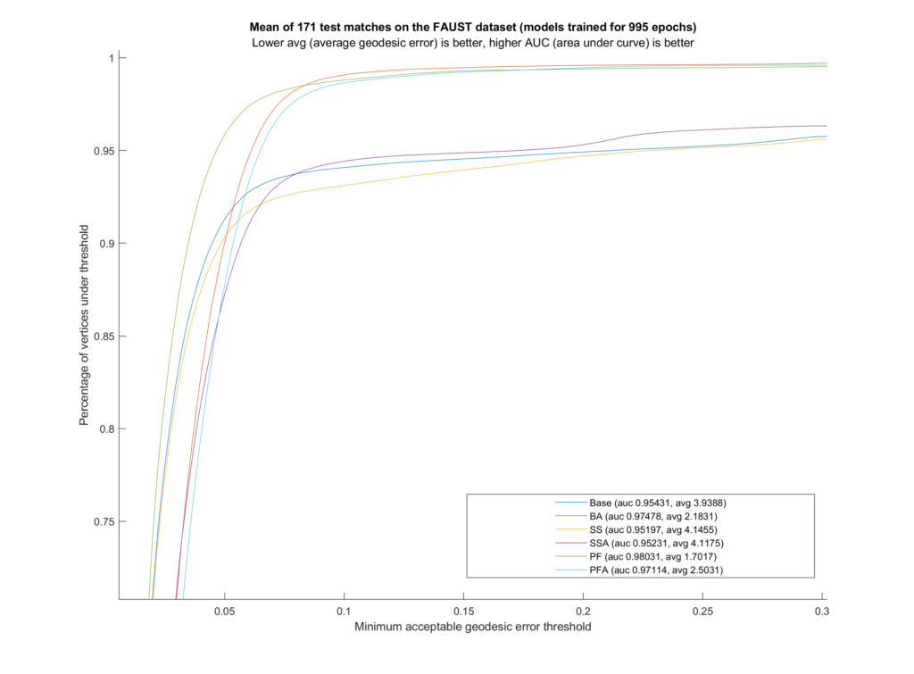
  4. Geodesic error: For evaluating our work, we use the metric of average geodesic error between the vertex-pair mappings predicted by our models and the ground truth vertex-pair indices provided with the dataset.

Result

We trained six different models on the FAUST dataset (which contains \(10\) human shapes at the same \(10\) poses each). Our training set includes \(81\) samples, leaving out one full shape (all of its \(10\) poses) and one full pose (so the network never sees any shape doing that pose). These remaining \(19\) inputs are the test set. Additionally, during testing we used ZoomOut by Melzi et al.

ModelData AugmentationContextual Loss
BaseFalseNone
BATrueNone
SSFalseSelf Similarity
SSATrueSelf Similarity
PFFalseProjected Features
PFATrueProjected Features
Table 1: We trained 7 models using the settings described in this table
Figure 2: The AUC (area under curve) curves and values with the average geodesic error for each model.

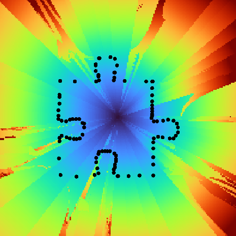
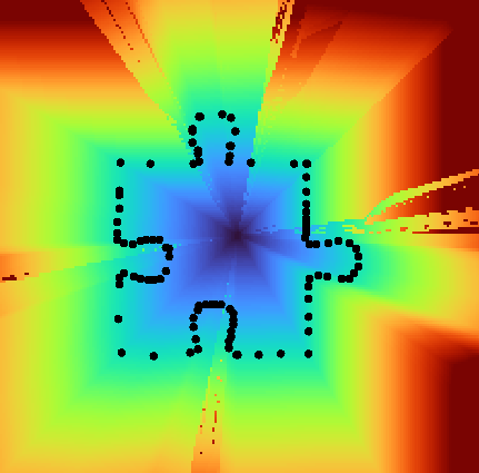
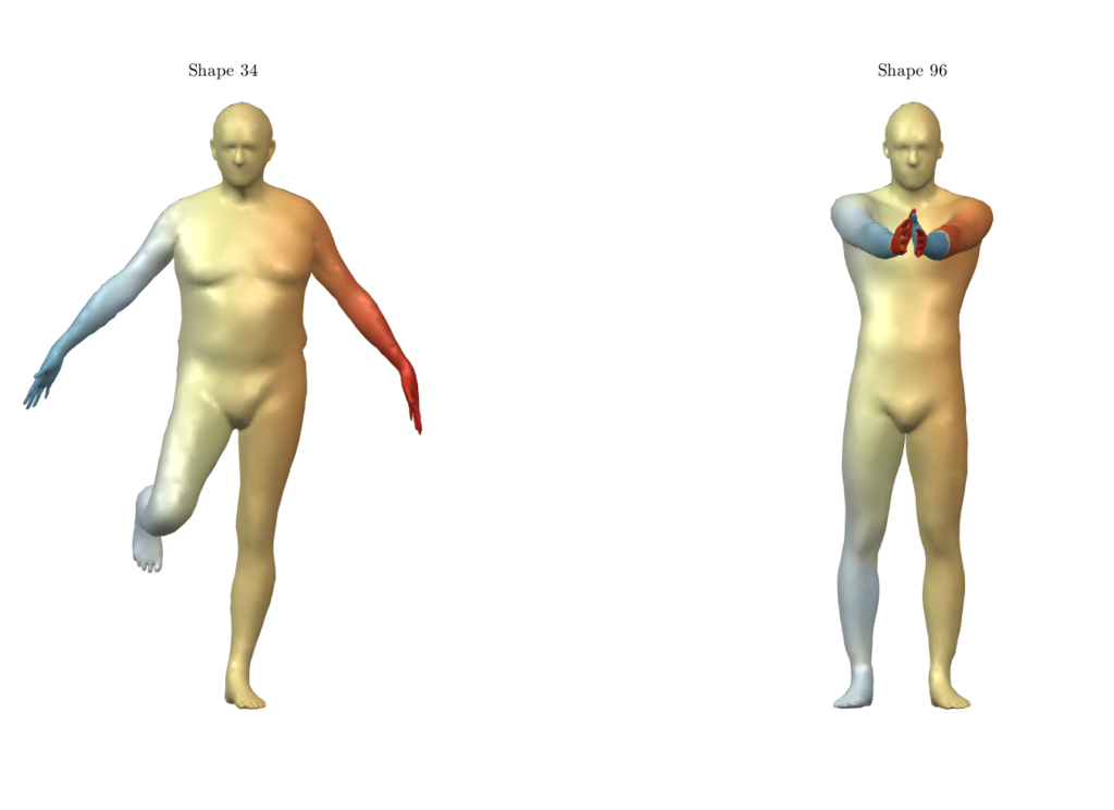
For qualitative comparison purposes, the following GIF displays a mapping result. Overall, the main noticeable visual differences between our work and the one we based ourselves on appeared when dealing with symmetric body parts (e.g., hands and feet).

Figure 3: Comparison between shape correspondence produced by the models described in Table 1.

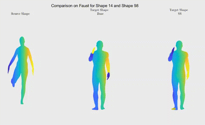
Still, as it can be seen, the symmetric body parts remain the less accurate mappings in our work too, meaning there’s still much to improve.

Conclusion

We thoroughly enjoyed working on this project during SGI and are looking forward to investigating this problem further, to which end we will continue to work on this project after the program. We want to extend our deepest gratitude to our mentor, Dr. Tal Shnitzer, for her continuous guidance and patience. None of this would be possible without her.

Thank you for taking the time to read this post. If there are any questions or suggestions, we’re eager to hear them!

Categories
Demo SGI research projects

Minimal Surfaces, But With Saddle Points

By Natasha Diederen, Alice Mehalek, Zhecheng Wang, and Olga Guțan

This week we worked on extending the results described here. We learned an array of new techniques and enhanced existing skills that we had developed the week(s) before. Here is some of the work we have accomplished since the last blog post. 

Tiling

One of the improvements we made was to create a tiling function which created an \( n^3 \) grid of our triply periodic surfaces, so that we were better able to visualise them as a structure. We started off with a surface inside a \( [-1, 1]^3 \) cube, and then imagined an \(n^3\) grid (pictured below). To make a duplicate of the surface in one of these grid cubes, we considered how much the surface would need to be translated in the \(x\), \(y\) and \(z\) directions. For example to duplicate the original surface in the black cube into the green square, we would need to shift all the \(x\)-coordinates in the mesh by two (since the cube is length two in all directions) and leave the \(y\)- and \(z\)-coordinates unchanged. Similarly, to duplicate the original surface into the purple square, we would need to shift the all \(x\)-coordinates in the mesh by two, all the \(y\)-coordinates by two, and all the \(z\)-coordinates by \(2n\).

Figure 1. A visualization of the the surface tiling.

To copy the surface \(n^3\) times into the right grid cubes, we need find all the unique permutations of groups of three vectors chosen from \((0,2,4, \dots, 2n)\) and add them to the vertices matrix of the of the mesh. To update the face data, we add multiples of the number of vertices each time we duplicate into a new cube. 

With this function in place, we can now see our triply periodic surfaces morphing as a larger structure.

Figure 2. A 3x3x3 Tiling of the Surface.

Blender

A skill we continued developing and something we have grown to enjoy, is what we affectionately call “blendering.” To speak in technical terms, we use the open-source software Blender to generate triangle meshes that we, then, use as tests for our code. 

For context: Blender is a free and open-source 3D computer graphics software tool set used for a plethora of purposes, such as creating animated films, 3D printed models, motion graphics, virtual reality, and computer games. It includes many features and it, truly, has endless possibilities. We used one small compartment of it: mesh creation and mesh editing, but we look forward to perhaps experiencing more of its possibilities in the future.

We seek to create shapes that are non-manifold; mathematically, this means that there exist local regions in our surface that are not homeomorphic to a subset of the Euclidean space. In other words, non-manifold shapes contain junctions where more than two faces meet at an edge, or more than two faces meet at a vertex without sharing an edge.

Figure 3. Manifold versus nonmanifold edges and vertices. Source.

This is intellectually intriguing to consider, because most standard geometry processing methods and techniques do not consider this class of shapes. As such, most algorithms and ideas need to be redesigned for non-manifold surfaces. 

Our Blender work consisted of a lot of trial-and-error. None of us had used Blender before, so the learning curve was steep. Yet, despite the occasional frustration, we persevered. With each hour worked, we increased our understanding and expertise, and in the end we were able to generate surfaces we were quite proud of. Most importantly, these triangle meshes have been valuable input for our algorithm and have helped us explore in more detail the differences between manifold and non-manifold surfaces. 

Figure 4. Manifold and Nonmanifold Periodic Surfaces.

Houdini

The new fellows joining this week came from a previous project on minimal surface led by Stephanie Wang, which used Houdini as a basis for generating minimal surfaces. Thus, we decided we could use Houdini to carry out some physical deformations, to see how non-manifold surfaces performed compared to similar manifold surfaces. 

We used a standard Houdini vellum solver with some modifications to simulate a section of our surface falling under gravity. Below are some of the simulations we created.

Figure 5. A Nonmanifold and a Manifold Surface Experiencing Gravity.

Newton’s Method

When we were running Pinkhall and Polthier’s algorithm on our surfaces, we noticed that that algorithm would not stop at a local saddle point such as the Schwarz P surface, but would instead run until there was only a thin strip of area left, which is indeed a minimum, but not a very useful one.

Therefore, we switched to Newton’s Method to solve our optimization problem.

We define the triangle surface area as an energy: let the three vertices of a triangle be \(\mathbf{q}_1\), \(\mathbf{q}_2\), \(\mathbf{q}_3\). Then \(E = \frac{1}{2} \|\mathbf{n}\| \), where \(\mathbf{n} = (\mathbf{q}_2-\mathbf{q}_1) \times (\mathbf{q}_3-\mathbf{q}_1)\) is the surface area normal. Then we derive its Jacobian and Hessian, and construct the Jacobian and Hessian for all faces in the mesh.

However, this optimization scheme still did not converge to the desired minimum, perhaps because our initialization is far from the solution. Additionally, one of our project mentors implemented the approach in C++ and, similarly, no results ensued. Later, we tried to add line search to Newton’s Method, but also no luck.

Although our algorithm still does not converge to some minimal surfaces which we know to exist, it has generated the following fun bugs.

Figure 6.
Figure 7.
Figure 8.

Future Work

In the previous blog post, we discussed studying the physical properties of nonmanifold TPMS. Over the past week, we used the Vellum Solver in Houdini and explored some of the differences in physical properties between manifold and nonmanifold surfaces. However, this is just the beginning — we can continue to expand our work in that direction.

Additional goals may include writing a script to generate many possible initial conditions, then converting the initial conditions into minimal surfaces, either by using the Pinkall and Polthier algorithm, or by implementing another minimal-surface-generating algorithm. 

More work can be done on enumerating all of the possible nonmanifold structures that the Pinkall and Polthier algorithm generates. The researchers can, then, categorize the structures based on their geometric or physical properties. As mentioned last week, this is still an open problem

Acknowledgments

We would like to thank our mentors Etienne Vouga, Nicholas Sharp, and Josh Vekhter for their patient guidance and the numerous hours they spent helping us debug our Matlab code, even when the answers were not immediately obvious to any of us. A special thanks goes to Stephanie Wang, who shared her Houdini expertise with us and, thus, made a lot of our visualizations possible. We would also like to thank our Teaching Assistant Erik Amezquita

Categories
Demo Math SGI research projects

Incompressible Flows on Meshes

An exploration of computational fluid dynamics

By: Natasha Diederen, Joana Portmann, Lucas Valença

These past two weeks, we have been working with Paul Kry to extend Jos Stam’s work on stable, incompressible fluid flow simulation. Stam’s paper Flows on Surfaces of Arbitrary Topology implements his stable fluid algorithm over patches of Catmull-Clark subdivision surfaces. These surfaces are ideal since they are smooth, can have arbitrary topologies, and have a quad patch parameterisation. However, Catmull-Clark subdivision surfaces are a quite specific class of surface, so we wanted to explore whether a similar algorithm could be implemented on triangle meshes to avoid the subdivision requirement.

Understanding basics of fluid simulation algorithms

We spent the first week of our project coming to terms with the different components of fluid flow simulation, which is based on solving the incompressible Navier-Stokes equation for velocities (1) and a similar advection-diffusion equation for densities (2) \[ \frac{\partial \mathbf{u}}{\partial t} = \mathbf{P} { -(\mathbf{u} \cdot \nabla)\mathbf{u} + \nu \nabla^2 \mathbf{u} + \mathbf{f} }, \quad (1)\] \[\frac{\partial \rho}{\partial t} = -(\mathbf{u} \cdot \nabla)\rho + \kappa \nabla^2 \rho + S, \quad (2)\] where \( \mathbf{u}\) is the velocity vector, \(t\) is time, \(\mathbf{P}\) is the projection operator, \( \nu\) is the viscosity coefficient, \(\mathbf{f}\) are external sources, \( \rho\) is the density scalar, \( \kappa\) is the diffusion coefficient, and \( S \) are the external sources. In the above equations, the Laplacian (often denoted \( \Delta\)) is written as \( \nabla^2\), as is usually done in works from the fluids community.

In his paper, Stam uses a splitting technique to deal with each term on its own. The algorithm carries out the following steps twice: first for the velocities and then for the densities (with no “project” step required for the latter). \[ \mathbf{u_0} {\underset{\overbrace{\text{add force}}^\text{ }}{\Rightarrow}} \mathbf{u_1} {\underset{\overbrace{\text{diffuse}}^\text{ }}{\Rightarrow}} \mathbf{u_2} {\underset{\overbrace{\text{advect}}^\text{ }}{\Rightarrow}} \mathbf{u_3} {\underset{\overbrace{\text{project}}^\text{ }}{\Rightarrow}} \mathbf{u_4} \]

Source: Flows on Surfaces of Arbitrary Topology

We start by adding any forces or sources we require. In the vector case, we can add acceleration forces such as gravity (which changes the velocities) or directly add velocity sources with a fixed location, direction, and intensity. In the scalar case, we add density sources that directly affect other quantities. 

Single density source pouring down with gravity over an initially zero velocity field

Densities and velocities are moved from a high to low concentration in the diffusion step, then moved along the vector field in the advection step. The final projection step ensures incompressible flow (i.e., that mass is conserved), using a Helmholtz-Hodge decomposition to force a divergence-free vector field. We will not go into much more detail on Stam’s original Stable Fluids solver. Dan Piponi’s Papers We Love presentation gives a very comprehensive introduction for those interested in learning more.

To better understand the square grid fluids solver, we implemented a MATLAB version of the C algorithm described in Stam’s paper Real-Time Fluid Dynamics for Games. In terms of implementation, since we were coding in MATLAB, we did not use the Gauss-Seidel algorithm (like Stam did) to solve the minimisation problems. Instead, we solved our own quadratic formulations directly. Although some of our methods differed from the original, the overall structure of the code remained the same.

Full simulation results over a square grid can be seen below. 

Generalising to triangle meshes

After a week, we understood the stable fluid algorithm well enough to extend it to triangle meshes. Stam’s paper for triangle meshes adapted the algorithm above from square grids to patches of a Catmull-Clark subdivided mesh, with the simulation boundary conditions at the edges of the parametric surfaces. We, on the other hand, wanted a method that would work over any triangular mesh, as long as such mesh, as a whole, is manifold without boundary. Moreover, we wished to do so by working directly with the triangles in the mesh without relying on subdivision surfaces for parameterisation. The main difference between our method and Stam’s was the need to deal with the varying angles between adjacent faces and their effect on advection, diffusion, and overall interpolation. In addition, since we’re working with manifolds without boundaries, we did not need to deal with boundary conditions (like in our 2D implementation). Furthermore, we had to choose between storing both vector and scalar quantities at the barycentre of each face or at each vertex. For simplicity, we chose the former.

What follows is a detailed explanation of how we implemented the three main steps of the fluid system: diffusion, advection and projection.

Diffusion

To diffuse quantities, we solved the equation\[ \dot{\mathbf{u}} = \nu \nabla^2 \mathbf{u},\] which can be discretised using the backwards Euler method for stability as follows \[ (\mathbf{I}-\Delta t \nu \nabla^2)\mathbf{u_2} = \mathbf{u_1}.\] Here, \( \mathbf{I} \) is the identity matrix and \( \mathbf{u_1}, \ \mathbf{u_2} \) are the respective original and final quantities for that iteration step, and can be either densities or vectors.

Surprisingly, this was far easier to solve for a triangle mesh than a grid due to the lack of boundary constraints. However, we needed to create our own Laplacian operators. They were used to deal with the transfer of density and velocity information from the barycentre of the current triangle to its three adjacent triangles. The first Laplacian we created was a linear operator that worked on vectors. For each face, before combining that face’s and its neighbours’ vectors with Laplacian weighting, it locally rotated the vectors lying on each of the face’s neighbouring faces. This way, the adjacent faces lay on the same plane as the central one. The rotated vectors were further weighted according to edge length (instead of area weighting) since we thought this would best represent flux across the boundary. The other Laplacian was a similar operator, but it worked on scalars instead of vectors. Thus, it involved weighting but not rotating the values at the barycentres (since they were scalars).

Diffusion of scalars over a flattened icosahedron
Advection

Advection was the most involved part of our code. To ensure the system’s stability, we implemented a linear backtrace method akin to the one in Stam’s Stable Fluids paper. Our approach considered densities and velocities as quantities currently stored at barycentres. It first looked at the current velocity at a chosen face then walked along the geodesic in the opposite direction (i.e., back in time). This allowed us to work out which location on the mesh we started at so that we would arrive at the current face one time-step later. This is analogous to Stam’s 2D walking over a square grid, interpolating quantities at the grid centres, but with a caveat. To walk the geodesics, we first had to use barycentric coordinates to work out the intersections with edges. Each time we crossed an edge, we rotated the walk direction vector from the current face to the next, making it as if we were walking along a plane. At the end of the geodesic, we obtain the previous position for the quantity on our current position. We then carried out a linear interpolation using barycentric coordinates and pre-interpolated vertex data. The result determined the previous value for the quantity in question. This quantity was then transported back to the current position. Vector quantities were also projected back onto the face plane at the end to account for any numerical inaccuracies that may have occurred.

Advection of a density blob over an icosahedron following gravity

Our advection code initially involved walking a geodesic for each mesh face, which is not computationally efficient in MATLAB. Thus, it accounted for the majority of the runtime of our code. The function was then mexed to C++, and the application now runs in real-time for moderately-sized meshes. 

Projection

So far, we have not guaranteed that diffusion and advection will result in incompressible flow. That is, the amount of fluid flowing into a point is the same as the amount of fluid flowing out. Hence, we need some way of creating such a field. According to the Helmholtz-Hodge decomposition, any vector field can be decomposed into curl-free and divergence-free fields, \[ \mathbf{w} = \mathbf{u} + \nabla q, \] where \( \mathbf{w}\) is the velocity field, \( \mathbf{u} \) is the divergence-free component, and \( \nabla q\) is the curl-free component.

A solution (for \(q\)) is implicitly found by solving a Poisson equation of the form \[ \nabla \cdot \mathbf{w} = \nabla^2 q\] where we used the cotangent Laplacian in gptoolbox for \(\nabla^2 q\). Subtracting the solution from the original vector field gives us the projection operator \( \mathbf{P}\) to find the divergence free component \( \mathbf{u} \) \[\mathbf{u} = \mathbf{Pw}=\mathbf{w}-\nabla q. \]

A uniform vector field before (left) and after (right) projection

This method works really nicely for our choice of having vector quantities stored at the faces. The pressures we get will be at the vertices. The gradients of those pressures are naturally computed at faces to alter the velocities to give an incompressible field. The only challenge is that the Laplacian is not full rank, so we need to regularise it by a small amount.

Future work

We would like to implement an alternative advection method, possibly more complicated. This method would involve interpolating vertex data and walking along mesh edges, rather than storing all our data in faces and walking geodesics crossing edges. This could possibly avoid extra blurring, which might be introduced by our current implementation. This occurs because we must first interpolate the data at the neighbouring barycenters to the vertices. This data is then used to do a second interpolation back to the barycentric coordinate the geodesic ends at.

For diffusion, although our method worked, there were a few things that could be improved upon. Mainly, diffusion did not look isotropic in cases with very thin triangles, which could be improved by an alternative to our current weighting of the Laplacian operator. Alternatively, we could use a more standard Laplacian operator if we stored quantities at the vertices instead of barycenters. This would result in more uniform diffusion at the expense of a more complicated advection algorithm.

Example of non-isotropic diffusion over a flattened torus

Conclusion

Final results

We would like to give a thousand thanks to Paul Kry for his mentorship. As a first foray into fluid simulations, this started as a very daunting project for us. Still, Paul smoothly led us through it by having dozens of very patient hours of Zoom calls, where we learned a lot about maths and coding (and biking in the rain). His enthusiasm for this project was infectious and is what enabled us to get everything working in such a short period. Still, even though we managed to get a good start on extending Stam’s methods to more general triangle meshes, there is a lot more work to do. Further extensions would focus on the robustness and speed of our algorithms, separation of face and vertex data, and incorporation of more components such as heat data or rotation forces. If anyone would like to view our work and play around with the simulations, here is the link to our GitHub repository. If anybody has any interesting suggestions about other possibilities to move forward, please feel free to reach out to us! 😉

Categories
Demo SGI research projects

Puzzle-ed

The SGI research program has been structured in a novel way in which each project lasts for one or two weeks only. This gives Fellows the opportunity to work with multiple mentors and in different areas of Geometry Processing. A lot of SGI fellows, including me, had wondered how we would be able to finish the projects in such a short period of time. After two weeks, as I pause my first research project at SGI, I am reminded of Professor Solomon’s remark that a surprising amount of work can be done within 1/2 weeks when guided by an expert mentor.

In this post, I have shared the work I have done under the mentorship of Prof. David Levin over the last two weeks.

Optimal Interlocking Parts via Implicit Shape Optimizations

In this project, we explored how to automatically design jigsaw puzzles such that all puzzle pieces are as close to a given input shape \(I\) as possible, while still satisfying the requirement of interlocking.

Lloyd relaxation with Shape Matching metric

As the first step, we needed a rough division of the domain into regions corresponding to puzzle pieces. For this initial division we used Lloyd’s relaxation as it ensured that the pieces would interlock. To create regions similar to the input shape, we employed a new distance metric. This metric is based on shape matching.

Shape Matching metric:

The input shape \(I\) is represented as a collection of points \(V\) on its boundary and is assumed to be of unit size and centered at the origin. Consider a pixel \(p\) and a site \(x\). First the input shape is translated to \(x\) ( \(V \rightarrow V’\)). The value of scaling factor \(s\) that minimizes the distance between \(p\) and the closest point \(V’_i\) on the boundary of the input shape gives us the shape matching metric. \[s^* = \text{arg min} \frac {1} {2}(dist(p, sV’))\]

Pre computing maps

The straightforward implementation for Lloyd’s relaxation that I had been using was iterative and therefore very slow. In fact, testing the algorithm for larger domains or complicated shapes that needed dense sampling of boundary points was infeasible. Therefore, optimizing the algorithm was an immediate requirement. I realized that relative to the site \(x\), the distances would vary around it in exactly the same way. So, computing the distance between each pixel and each site separately during each iteration of Lloyd’s relaxation was redundant and could be avoided by pre-computing a distance map for the given object before starting Lloyd’s relaxation.

Enhancing the shape matching metric

In addition to speeding up the algorithm, the distance maps also helped in determining the next step. As can be seen from the figures above, the maps weren’t smooth. These jumps in distance fields occurred because the shape matching metric worked on a set of discrete points. Optimizing the scaling factor for minimizing distance to the closest edge instead of closest point resolved this.

200×200 Map with enhanced Shape Matching metric input shape of a puzzle piece.

Shaping the puzzle pieces (In progress)

The initial regions are obtained from Lloyd’s algorithm with the shape matching metric need to be refined so that the final puzzle pieces are highly similar to the input shape \(I\).

I am currently exploring the use of point set registration methods to find the best transformations on the input shape so that it fits the initial regions. These transformations could then be used to inform the next iteration of Lloyd’s algorithm to refine the regions. This process can be repeated until the region stops changing, giving us our final puzzle pieces.

I have thoroughly enjoyed working on this project, and I am looking forward to the next project I would be working on!

Categories
Demo News

Before the Beginning

While the official start date, 19th of July, is still a couple of days from now, the SGI experience began the very day I received the acceptance letter back in March. In this post I briefly share my thoughts on the journey so far – SGI’s social event, attending the Symposium on Geometry Processing 2021, and my implementation of a paper presented in the conference.

Slack and Virtual Coffees

The SGI slack channel was created at the end of March and has been buzzing with activity ever since. Initially, as everyone introduced themselves, I was proud to see that I am a part of a team that is truly diverse in every aspect – geographically, racially, religiously and even by educational backgrounds!

Shortly after, we started biweekly ‘virtual coffees’ in which two people were randomly paired up to meet. These sessions have been instrumental in refining my future goals. As someone who entered research just as the world closed down and started working from home, I haven’t had the opportunity to visit labs and chat with graduate students during the lunch break or by that water cooler. Speaking with professors, teaching assistants and SGI Fellows has debunked many of my misconceptions regarding graduate school.  Additionally, I also learned a lot about possible career paths in geometry processing and adjacent fields like computer graphics, and about the culture in this community.

Symposium on Geometry Processing

SGP was a comprehensive four-day event including tutorials, paper presentations and talks on the latest research in the field. While all the sessions were amazing, I was especially awed by the keynote ‘Computing Morphing Matter’ by Professor Lining Yao from Carnegie Mellon University. She talked about various techniques that combine geometry, physics, and material science to create objects that can change shape in a pre-determined manner. This ability to morph can be leveraged in various ways and across many industries. To list a few of its usages, it can be used to create a compact product that can morph into the final shape later thus saving packaging material and shipping costs, to develop self-locking mechanisms, and to produce aesthetically appealing shapes. Due to such varied use cases, morphing matter has applications in furniture designing to food production to engineering problems.

Implementing ‘Normal-Driven Spherical Shape Analogies’

In one section of the tutorial ‘An Introduction to Geometry Processing Programming in MATLAB with gptoolbox’ at SGP, the ease with which complex problems can be solved using MATLAB and gptoolbox was demonstrated by implementing research papers. I had never before seen a language/library tutorial that included paper implementations and was delighted at the prospect of turning the tedious process of learning a new tool into an exciting process of implementing a research paper. Eager to test out this new way, I implemented one of the research papers presented at the SGP – ‘Normal-Driven Spherical Shape Analogies’ by Hsueh-Ti Derek Liu and Alec Jacobson.

The paper details how an input shape can be stylized to look like a target shape by using normal driven shape analogies. The process boils down to three steps:

  1. Compute the mapping between a sphere and the target shape.
  2. Using the sphere-target shape mapping as an analogy, find the target normals for the input object.
  3. Generate the stylized output by deforming the input object to approximate the target normals.

When I arrived at code that gave outputs that looked right, I faced an unanticipated problem: Without any error metric, how can you know that it’s working well? After working on this project I definitely have a renewed appreciation for work in stylization.