During the 4th week of SGI, we worked closely with Dr. Tal Shnitzer to develop an improved loss function for learning functional maps with robustness to symmetric ambiguity. Our project goal was to modify recent weakly-supervised works that generated deep functional maps to make them handle symmetric correspondences better.
Introduction:
Shape correspondence is a task that has various applications in geometry processing, computer graphics, and computer vision – quad mesh transfer, shape interpolation, and object recognition, to name a few. It entails computing a mapping between two objects in a geometric dataset. Several techniques for computing shape correspondence exist – functional maps is one of them.
A functional map is a representation that can map between functions on two shapes’ using their eigenbases or features (or both). Formally, it is the solution to \(\mathrm{arg}\min_{C_{12}}\left\Vert C_{12}F_1-F_2\right\Vert^2\), where \(C_{12}\) is the functional map from shape \(1\) to shape \(2\) and \(F_1\), \(F_2\) are corresponding functions projected onto the eigenbases of the two shapes, respectively.
Therefore, there is no direct mapping between vertices in a functional map. This concise representation facilitates manipulation and enables efficient inference.
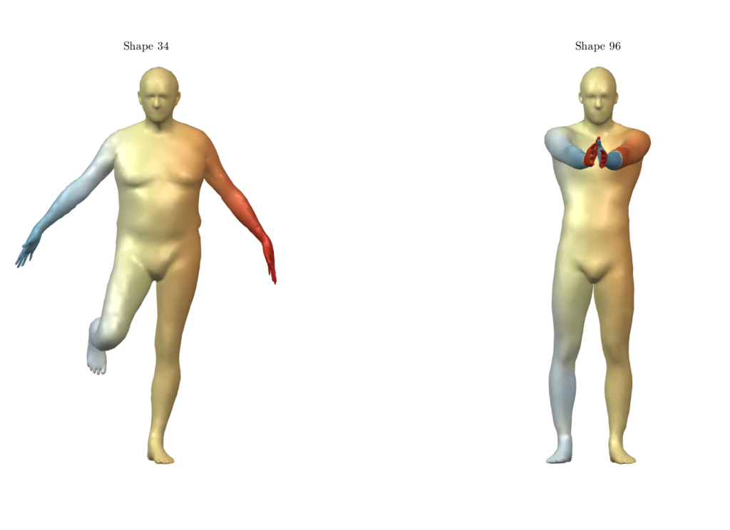
Figure 1: The approach proposed by Sharma and Ovsjanikov may fail on symmetric regions. Notice the hands, which have not been matched correctly due to their symmetric structure.
Recently, unsupervised deep learning methods have been developed for learning functional maps. One of the main challenges in such shape correspondence tasks is learning a map that differentiates between shape regions that are similar (due to symmetry). We worked on tackling this challenge.
Background
We build upon the state-of-the-art work “Weakly Supervised Deep Functional Map for Shape Matching” by Sharma and Ovsjanikov, which learns shape descriptors from raw 3D data using a PointNet++ architecture. The network’s loss function is based on regularization terms that enforce bijectivity, orthogonality, and Laplacian commutativity.
This method is weakly supervised because the input shapes must be equally aligned, i.e., share the same 6DOF pose. This weak supervision is required because PointNet-like feature extractors cannot distinguish between left and right unless the shapes share the same pose.
To mitigate the same-pose requirement, we explored adding another component to the loss function Contextual Loss by Mechrez et al. Contextual Loss is high when the network learns a large number of similar features. Otherwise, it is low. This characteristic promotes the learning of global features and can, therefore, work on non-aligned data.
Work
Model architecture overview: As stated above, our basic model architecture is similar to “Weakly Supervised Deep Functional Map for Shape Matching” by Sharma and Ovsjanikov. We use the basic PointNet++ architecture and pass its output through a \(4\)-layer ResNet model. We use the output from ResNet as shape features to compute the functional map. We randomly select \(4000\) vertices and pass them as input to our PointNet++ architecture.
Data augmentation: We randomly rotated the shapes of the input dataset around the “up” axis (in our case, the \(y\) coordinate). Our motivation for introducing data augmentation is to make the learning more robust and less dependent on the data orientation.
Contextual loss: We explored two ways of adding contextual loss as a component:
Self-similarity: Consider a pair of input shapes (\(S_1\), \(S_2\)) of features \(P_1\) with \(P_2\) respectively. We compute our loss function as follows: \(L_{CX}(S_1, S_2) = -log(CX(P_1, P_1)) – log(CX(P_2, P_2))\), where \(CX(x, y)\) is the contextual similarity between every element of \(x\) and every element of \(y\), considering the context of all features in \(y\). More intuitively, the contextual loss is applied on each shape feature with itself (\(P_1\) with \(P_1\) and \(P_2\) with \(P_2\)), thus giving us a measure of ‘self-similarity’ in a weakly-supervised way. This measure will help the network learn unique and better descriptors for each shape, thus alleviating errors from symmetric ambiguities.
Projected features: We also explored another method for employing the contextual loss. First, we project the basis \(B_1\) of \(S_1\) onto \(S_2\), so that \(B_{12} = B_ 1 \cdot C_{12}\). Similarly, \(B_{21} = B_2 \cdot C_{21}\). Note that the initial bases \(B_1\) and \(B_2\) are computed directly from the input shapes. Next, we want the projection \(B_{12}\) to get closer to \(B_2\) (the same applies for \(B_{21}\) and \(B_1\)). Hence, our loss function becomes: \(L_{CX}(S_1, S_2) = -log(CX(B_{21}, B_1)) – log(CX(B_{12}, B_2))\). Our motivation for applying this loss function is to reduce symmetry error by encouraging our model to map the eigenbases using \(C_{12}\) and \(C_{21}\) more accurately.
Geodesic error: For evaluating our work, we use the metric of average geodesic error between the vertex-pair mappings predicted by our models and the ground truth vertex-pair indices provided with the dataset.
Result
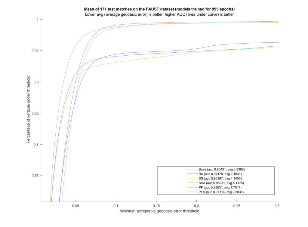
We trained six different models on the FAUST dataset (which contains \(10\) human shapes at the same \(10\) poses each). Our training set includes \(81\) samples, leaving out one full shape (all of its \(10\) poses) and one full pose (so the network never sees any shape doing that pose). These remaining \(19\) inputs are the test set. Additionally, during testing we used ZoomOut by Melzi et al.
Model
Data Augmentation
Contextual Loss
Base
False
None
BA
True
None
SS
False
Self Similarity
SSA
True
Self Similarity
PF
False
Projected Features
PFA
True
Projected Features
Table 1: We trained 7 models using the settings described in this table
Figure 2: The AUC (area under curve) curves and values with the average geodesic error for each model.
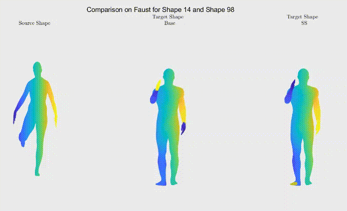
For qualitative comparison purposes, the following GIF displays a mapping result. Overall, the main noticeable visual differences between our work and the one we based ourselves on appeared when dealing with symmetric body parts (e.g., hands and feet).
Figure 3: Comparison between shape correspondence produced by the models described in Table 1.
Still, as it can be seen, the symmetric body parts remain the less accurate mappings in our work too, meaning there’s still much to improve.
Conclusion
We thoroughly enjoyed working on this project during SGI and are looking forward to investigating this problem further, to which end we will continue to work on this project after the program. We want to extend our deepest gratitude to our mentor, Dr. Tal Shnitzer, for her continuous guidance and patience. None of this would be possible without her.
Thank you for taking the time to read this post. If there are any questions or suggestions, we’re eager to hear them!
Over the first 2 weeks of SGI (July 26 – August 6, 2021), we have been working on the “Probabilistic Correspondence Synchronization using Functional Maps” project under the supervision of Nina Miolane and Tolga Birdal with TA Dena Bazazian. In this blog, we motivate and formulate our research questions and present our first results.
Finding a meaningful correspondence between two or more shapes is one of the most fundamental shape analysis tasks. Van Kaick et al (2010) stated the problem as follows: given input shapes \(S_1, S_2,…, S_N\), find a meaningful relation (or mapping) between their elements. Shape correspondence is a crucial building block of many computer vision and biomedical imaging algorithms, ranging from texture transfer in computer graphics to segmentation of anatomical structures in computational medicine. In the literature, shape correspondence has been also referred to as shape matching, shape registration, and shape alignment.
In this project, we consider a dataset of 3D shapes and represent the correspondence between any two shapes using the concept of “functional maps” [see section 1]. We then show how the technique of “synchronization” [see section 2] allows us to improve our computations of shape correspondences, i.e., allows us to refine some initial estimates of functional maps. During this project, we implement a method of synchronization using tools from geometric statistics and optimization on a Riemannian manifold describing functional maps, the Stiefel manifold, using the packages geomstats and pymanopt.
1. Representing Shape Correspondences with Functional Maps
Shape correspondence is a well-studied problem that applies to both rigid and non-rigid matching. In the rigid scenario, the transformation between two given 3D shapes can be described by a 3D rotation and a 3D translation. If there is a non-rigid transformation between the two 3D shapes, we can use point-to-point correspondences to model the shape matching. However, as mentioned in Ovsjanikov et al (2012), many practical situations make it either impossible or unnecessary to establish point-to-point correspondences between a pair of shapes, because of inherent shape ambiguities or because the user may only be interested in approximate alignment. To tackle that problem, functional maps are introduced in Ovsjanikov et al (2012) and can be considered a generalization of point-to-point correspondences.
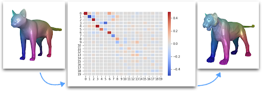
By definition, a functional map between two shapes is a map between functions defined on these shapes. A function defined on a shape assigns a value to each point of the shape and can be represented as a heatmap on the shape; see Figure 2 for functions defined on a cat and a tiger respectively. Then, the functional map of Figure 2 maps the function defined on the first shape — the cat — to a function on the second shape — the tiger. All in all, instead of computing correspondences between points on the shapes, functional maps compute mappings between functions defined on the shapes.
In practice, the functional map is represented by a \(p \times q\) matrix, called C. Specifically, we consider p basis functions defined on the source shape (e.g. the cat) and q basis functions defined on the target shape (e.g. the tiger). Typically, we can consider the eigenfunctions of the Laplace-Beltrami operator. The functional map C then represents how each of the p basis functions of the source shape is mapped onto the set of q basis functions of the target shape.
Figure 2: Functional map mapping a function defined on a cat (“source shape”) to a function defined on a tiger (“target shape”). The functional map is represented by a matrix that describes how each of the 20 basis functions chosen on the source shape is mapped onto the set of 20 basis functions chosen on the target shape. (generated using PyFM)
2. Problem Formulation: Synchronization Improves Shape Correspondences
In this section, we describe the technique of “synchronization” that allows us to improve the computations of functional maps between shapes, and we introduce the related notations. We use subsets of the TOSCA dataset (http://tosca.cs.technion.ac.il/book/resources_data.html), which contains a dataset of 3D shapes of cats, to illustrate the concepts.
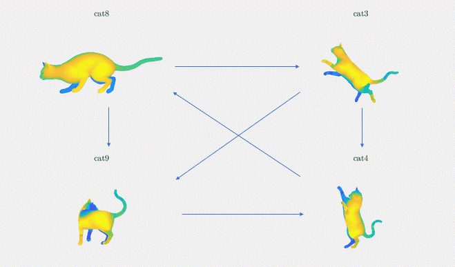
Intuitively, the method of synchronization builds a graph that links pairs of 3D shapes within the input dataset by edges representing their functional maps; see Figure 3 for an example of such a graph with 4 shapes and 6 edges. The method of synchronization then leverages the property of cycle consistency within the graph. Cycle consistency is a concept that enforces a global agreement among the shape matchings in the graph, by distributing and minimizing the errors to the entire graph — so that not only pairwise relationships are modeled but also global ones. This is why, intuitively, synchronization allows us to refine the functional maps between pairs of shapes by extracting global information over the entire shape dataset.
Let’s now introduce notations to give the mathematical formulation of the synchronization method. We begin with a set of pairwise functional maps, \(C_{ij} \in \{\mathcal{F}(M_i,M_j)\}_{i,j}\) for \((i,j) \in \varepsilon\). M denotes the set of \(n\) input 3D shapes and \(\varepsilon\) denotes the set of the edges of the directed graph of \(n\) nodes representing the shapes: \(\varepsilon \subset \{1,\dots, n\} \times \{1,\dots, n\}\). We are then interested in finding the underlying “absolute functional maps” \(C_i\) for \(i\in\{1,\dots,n\}\) with respect to a common origin (e.g. \(C_0=I\), the identity matrix) that would respect the consistency of the underlying graph structure. We illustrate these notations in Figure 3. Given a graph of four cat shapes (cat8, cat3, cat9, cat4) and their relative functional maps (C83, C94, C34, C89, C48, C39), we want to find the absolute functional maps (C8, C3, C4, C9).
Figure 3: Synchronization between four shapes from the TOSCA dataset. We are given the functional maps Cij between pairs of shapes (i, j) in the graph. We wish to find the absolute functional map of these shapes: the Ci for each shape i in the graph.
3. Riemannian Optimization Algorithm
In this section, we explain how we frame the synchronization problem as an optimization problem on a Riemannian manifold.
Constraints: As shown by Ovsjanikov et al (2012), functional maps are orthogonal matrices for near-isometry: the columns forming functional map matrix C are orthonormal vectors. Hence, functional maps naturally reside on the Stiefel manifold which is the manifold of matrices with orthonormal columns. The Stiefel manifold can be equipped with a Riemannian geometric structure that is implemented in the packages geomstats and pymanopt. We design a Riemannian optimization algorithm that iterates over the Stiefel manifold (or power manifold of Stiefels) using elementary operations of Riemannian geometry, and converges to our estimates of absolute functional maps. Later, we compare this method to the corresponding non-Riemannian optimization algorithm that does not constrain the iterates to belong to the Stiefel manifold.
Cost function: We describe here the cost function associated with the Riemannian optimization. We want our absolute functional maps to be consistent with the relative maps as much as possible. That is, in the ideal case, \(C_i \cdot C_{ij} = C_j \). To abide by this, we consider the following cost function in our algorithm:
In this equation, we measure this norm in terms of the Frobenius norm, which is equal to the square root of the sum of the squares of the matrix values. This cost is implemented in Python, as follows:
# Cis are the maps we compute, input_Cijs are the input functional maps
def cost_function(Cis, input_Cijs):
    cost = 0.
    for edge, Cij in zip(EDGES, input_Cijs):
        i, j = edge
        Ci_Cij = np.matmul(Cis[i], Cij)
        cost += np.linalg.norm(Ci_Cij - Cis[j], "fro") ** 2
return cost
Optimizer: Our goal is to minimize this cost with respect to the Cis, while constraining the Cis to remain on the Stiefel manifold. For solving our optimization problem, we use the TrustRegion algorithm from the Pymanopt library.
4. Experiments and Results
We present some preliminary results on the TOSCA dataset.
Dataset: For our baseline experiments, we use the 11 cat shapes from the TOSCA dataset. The cats have a wide variety of poses and deformations which make them particularly suitable for our baseline testing.
Initial Functional Map Generation: For each pair of cats within the TOSCA dataset, we compute initial functional maps using state-of-the-art methods, by adapting the source code from here. Our functional maps are of size 20 * 20, i.e they are written in terms of 20 basis functions on the source shape and 20 basis functions on the target shape.
Graph Generation: We implement a random graph generator using networkX that can generate cycle-consistent graphs. We use this graph generator to generate a graph, with nodes corresponding to shapes from a subset of the TOSCA dataset, and with edges depicting the correspondence relationship between the selected shapes. In our future experiments, this graph generator will allow us to compare the performance of our method depending on the number of shapes (or nodes) and the number of known initial correspondences (or initial functional maps) between the shapes (or sparsity of the graph).
Perturbation: We showcase the efficiency of our algorithm by inducing a synthetic perturbation on the initial functional maps and showing how synchronization allows us to correct it. Specifically, we add a Gaussian perturbation to the initial functional maps, with standard deviation s = 0.1, and project the resulting corrupted matrices on the Stiefel manifold to get “corrupted functional maps”. The corrupted functional maps are the inputs of our optimization algorithm.
Results: We demonstrate the result of our optimization algorithm for a subset of the TOSCA dataset and initial (corrupted) functional maps generated with the methods described above: we consider the graph with 4 shapes and 6 edges that was presented in Figure 3. The optimization algorithm converged in less than 20 iterations and less than 1 second. Figure 4 shows the output of our optimization algorithm on this graph. Specifically, we consider a function defined on one of the cats, and map it to the other cats using our functional maps. We can see how efficiently different body parts are being meaningfully mapped in each of these cat shapes.
Figure 4. The absolute functional map output is visualized as point-to-point mapping, The regions marked with the same colors on the four shapes are being mapped to each other (noise standard deviation = 0.1)
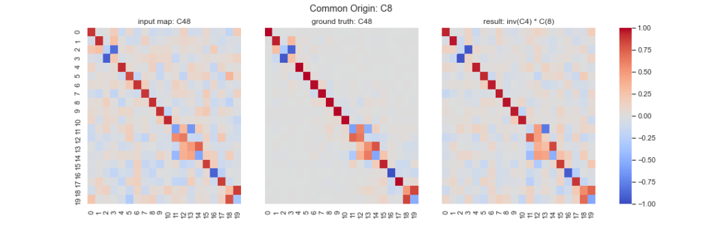
Comparison with initially corrupted functional maps: We show how synchronization allows us to improve over our initially corrupted functional maps. Figure 5 shows a comparison between the corrupted functional maps, the ground-truth (un-corrupted) functional maps, and the output functional maps computed via the output absolute maps given by our algorithm, for the correspondence between cat 4 and cat 8. While the algorithm does not allow to fully recover the ground-truth, our analysis shows that it has refined the initially corrupted functional maps. For example, we observe that the noise has been reduced for the off-diagonal elements. This visual inspection is confirmed quantitatively: the distance between the initially corrupted functional maps and the ground-truth is 2.033 while the distance between the output functional maps and the ground-truth is 1.853, as observed in Table 1.
However, the results on the other functional maps C83, C39, C94, C89, C34 are less convincing; see errors reported in Table 1. This can be explained by the fact that we have chosen a relatively small graph, with only 4 nodes i.e. 4 shapes. As a consequence, the synchronization method leveraging cycle consistency can be less efficient. Future results will investigate the performances of our approach for different graphs with different numbers of nodes and different numbers of edges (sparsity of the graph).
Func. Maps.
Error C83
Error C39
Error C48
Error C94
Error C89
Error C34
Before sync.
1.762
1.658
2.033
1.877
1.819
1.854
After sync.
1.659
2.519
1.741
2.323
2.118
2.492
After sync. (Riem.)
2.576
2.621
1.853
1.984
2.181
2.519
Table 1. Frobenius norms of the difference between different functional maps and the ground-truth functional maps
Discussion: We compare this method with the method that does not restrict the functional maps to be on the Riemannian Stiefel manifold. We observe similar performances, with a preference for the non-Riemannian optimization method. Future work will investigate which data regimes require optimization with Riemannian constraints and which regimes do not necessarily require it.
Figure 5. Result for the functional map relating cat 4 to cat 8. Left: Corrupted functional maps that are the inputs of our algorithm. Middle: ground-truth functional maps, i.e. functional maps before corruption with synthetic noise. Right: Functional maps given by the output of our algorithm.
Conclusion
In this blog, we explained the first steps of our work on shape correspondences. Currently, we are working on a Markov Chain Monte Carlo (MCMC) implementation to get better results with associated uncertainty quantification. We are also working on a custom gradient function to get better performance. In the coming weeks, we look forward to experimenting with other benchmark datasets and comparing our results with baselines.
Acknowledgment: We thank our mentors, Dr. Nina Miolane and Dr. Tolga Birdal for their consistent guidance and mentorship. They have relentlessly supported us from the beginning, debugged our errors. We especially thank Nina for guiding us to write this blog post. We are very grateful for her keen enthusiasm 😇. We also thank our TA, Dr. Dena Bazazian for her important feedback.