Categories
Demo SGI research projects

Minimal Surfaces, But With Saddle Points

By Natasha Diederen, Alice Mehalek, Zhecheng Wang, and Olga Guțan

This week we worked on extending the results described here. We learned an array of new techniques and enhanced existing skills that we had developed the week(s) before. Here is some of the work we have accomplished since the last blog post. 

Tiling

One of the improvements we made was to create a tiling function which created an \( n^3 \) grid of our triply periodic surfaces, so that we were better able to visualise them as a structure. We started off with a surface inside a \( [-1, 1]^3 \) cube, and then imagined an \(n^3\) grid (pictured below). To make a duplicate of the surface in one of these grid cubes, we considered how much the surface would need to be translated in the \(x\), \(y\) and \(z\) directions. For example to duplicate the original surface in the black cube into the green square, we would need to shift all the \(x\)-coordinates in the mesh by two (since the cube is length two in all directions) and leave the \(y\)- and \(z\)-coordinates unchanged. Similarly, to duplicate the original surface into the purple square, we would need to shift the all \(x\)-coordinates in the mesh by two, all the \(y\)-coordinates by two, and all the \(z\)-coordinates by \(2n\).
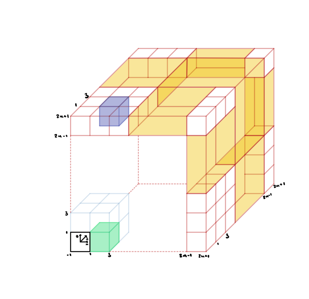
Figure 1. A visualization of the the surface tiling.

To copy the surface \(n^3\) times into the right grid cubes, we need find all the unique permutations of groups of three vectors chosen from \((0,2,4, \dots, 2n)\) and add them to the vertices matrix of the of the mesh. To update the face data, we add multiples of the number of vertices each time we duplicate into a new cube. 

With this function in place, we can now see our triply periodic surfaces morphing as a larger structure.

Figure 2. A 3x3x3 Tiling of the Surface.

Blender

A skill we continued developing and something we have grown to enjoy, is what we affectionately call “blendering.” To speak in technical terms, we use the open-source software Blender to generate triangle meshes that we, then, use as tests for our code. 

For context: Blender is a free and open-source 3D computer graphics software tool set used for a plethora of purposes, such as creating animated films, 3D printed models, motion graphics, virtual reality, and computer games. It includes many features and it, truly, has endless possibilities. We used one small compartment of it: mesh creation and mesh editing, but we look forward to perhaps experiencing more of its possibilities in the future.

We seek to create shapes that are non-manifold; mathematically, this means that there exist local regions in our surface that are not homeomorphic to a subset of the Euclidean space. In other words, non-manifold shapes contain junctions where more than two faces meet at an edge, or more than two faces meet at a vertex without sharing an edge.
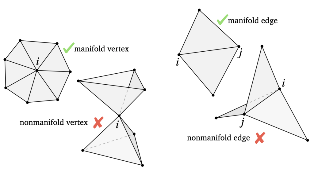
Figure 3. Manifold versus nonmanifold edges and vertices. Source.

This is intellectually intriguing to consider, because most standard geometry processing methods and techniques do not consider this class of shapes. As such, most algorithms and ideas need to be redesigned for non-manifold surfaces. 

Our Blender work consisted of a lot of trial-and-error. None of us had used Blender before, so the learning curve was steep. Yet, despite the occasional frustration, we persevered. With each hour worked, we increased our understanding and expertise, and in the end we were able to generate surfaces we were quite proud of. Most importantly, these triangle meshes have been valuable input for our algorithm and have helped us explore in more detail the differences between manifold and non-manifold surfaces. 

Figure 4. Manifold and Nonmanifold Periodic Surfaces.

Houdini

The new fellows joining this week came from a previous project on minimal surface led by Stephanie Wang, which used Houdini as a basis for generating minimal surfaces. Thus, we decided we could use Houdini to carry out some physical deformations, to see how non-manifold surfaces performed compared to similar manifold surfaces. 

We used a standard Houdini vellum solver with some modifications to simulate a section of our surface falling under gravity. Below are some of the simulations we created.

Figure 5. A Nonmanifold and a Manifold Surface Experiencing Gravity.

Newton’s Method

When we were running Pinkhall and Polthier’s algorithm on our surfaces, we noticed that that algorithm would not stop at a local saddle point such as the Schwarz P surface, but would instead run until there was only a thin strip of area left, which is indeed a minimum, but not a very useful one.

Therefore, we switched to Newton’s Method to solve our optimization problem.

We define the triangle surface area as an energy: let the three vertices of a triangle be \(\mathbf{q}_1\), \(\mathbf{q}_2\), \(\mathbf{q}_3\). Then \(E = \frac{1}{2} \|\mathbf{n}\| \), where \(\mathbf{n} = (\mathbf{q}_2-\mathbf{q}_1) \times (\mathbf{q}_3-\mathbf{q}_1)\) is the surface area normal. Then we derive its Jacobian and Hessian, and construct the Jacobian and Hessian for all faces in the mesh.

However, this optimization scheme still did not converge to the desired minimum, perhaps because our initialization is far from the solution. Additionally, one of our project mentors implemented the approach in C++ and, similarly, no results ensued. Later, we tried to add line search to Newton’s Method, but also no luck.

Although our algorithm still does not converge to some minimal surfaces which we know to exist, it has generated the following fun bugs.

Figure 6.
Figure 7.
Figure 8.

Future Work

In the previous blog post, we discussed studying the physical properties of nonmanifold TPMS. Over the past week, we used the Vellum Solver in Houdini and explored some of the differences in physical properties between manifold and nonmanifold surfaces. However, this is just the beginning — we can continue to expand our work in that direction.

Additional goals may include writing a script to generate many possible initial conditions, then converting the initial conditions into minimal surfaces, either by using the Pinkall and Polthier algorithm, or by implementing another minimal-surface-generating algorithm. 

More work can be done on enumerating all of the possible nonmanifold structures that the Pinkall and Polthier algorithm generates. The researchers can, then, categorize the structures based on their geometric or physical properties. As mentioned last week, this is still an open problem

Acknowledgments

We would like to thank our mentors Etienne Vouga, Nicholas Sharp, and Josh Vekhter for their patient guidance and the numerous hours they spent helping us debug our Matlab code, even when the answers were not immediately obvious to any of us. A special thanks goes to Stephanie Wang, who shared her Houdini expertise with us and, thus, made a lot of our visualizations possible. We would also like to thank our Teaching Assistant Erik Amezquita

Categories
Geometry processing Math

When Algorithms Go Wrong

By Natasha Diederen, Sahra Yusuf, and Olga Guțan

I. Introduction

An algorithm is a finite sequence of well-defined, computer-implementable instructions, typically designed to solve a class of specific problems or to perform a computation. Similarly to how we use our brains to (sometimes wrongly) categorize things in order to make sense of the world, a computer needs an algorithm to make sense of what the user is asking it to do. Since an algorithm is a way of communication between two vastly different entities — a human and a machine — some information gets lost along the way. The process is intellectually intriguing to witness, however, problems can arise when we use algorithms to make decisions that influence the lives of humans and other self-aware living beings. 

Algorithms are indispensable for efficiently processing data; therefore they will continue to be part of our programming ecosystem. However, we can (and must) keep some space in our minds for the additional nuances that reality contains. While a programmer may not be able to fully convey these nuances to a computer, we must be aware that no algorithm’s output is final, all-encompassing, and universally true. Furthermore, we must be mindful of the conclusions we draw from the output of algorithms. 

II. Algorithms Gone Wrong

Broadly speaking, potential pitfalls for algorithms are manifold. The issues stem from the nature of the algorithms — a communication tool between a human entity and a nonhuman entity (a computer).  These problems morph into different real-life issues based on what types of algorithms we use and what we use them for. 

Even when playing with algorithms intended to solve toy problems that we already have the answers to, we can notice errors. However, in real life, data is (even) more messy and consequences are far larger. In 2018, Elaine Herzberg was hit and killed by a self-driving taxi. She was jaywalking in the dark with a bicycle by her side and the car alternated between classifying her as a person and a bicycle, thus miscalculating her trajectory and not classifying Elaine as an obstruction. In this case, the safety driver was distracted by a television program, and thus not entirely blameless. However, this serves as an example of how our blind trust in the reliability of algorithms can often result in complacency, with far reaching consequences. 

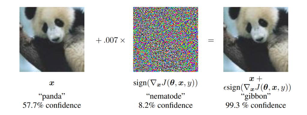
A further example of error in algorithms is adversarial attacks on neural networks. This is when researchers (or hackers) feed a neural network a modified image, where changes made to the image are imperceptible to the human eye. Nevertheless, this can result in incorrect classification by neural networks, with high confidence to boot. 

Figure 1. A demonstration of fast adversarial example generation applied to GoogLeNet (Szegedy et al., 2014a) on ImageNet. Source.

In Figure 1 we see how by adding an imperceptibly small vector whose elements are equal to the sign of the elements of the gradient of the cost function with respect to the input, we can change GoogLeNet’s classification of the image. Here the \(\epsilon\) of 0.007 corresponds to the magnitude of the smallest bit of an 8 bit image encoding after GoogLeNet’s conversion to real numbers.

Although researchers are working on making neural networks more robust to these sorts of attacks, susceptibility to adversarial attacks seems to be an inherent weakness of deep neural networks. This has serious security implications as computer vision increasingly relies on these models for facial recognition, autonomous vehicles, speech recognition and much more. 

III. Geometry Processing with Imperfect Data

In geometry processing, there is often a need for refinement of geometric data, especially when the data is taken from “real” contexts. Examples of imperfections in 3D models include gaps, self-intersections, and non-manifold geometry, or geometry which cannot exist in reality (e.g. edges included in more than two faces and disconnected vertices).

One common source of imperfect, “real-life” data is 3D object scanning. The resulting models typically include gaps and large self-intersections as a result of incomplete scanning or other error arising from the scanning method. Despite these significant problems, scanned data is still invaluable for rapidly generating assets for use in game development and other applications. During our time at the Summer Geometry Institute, Dr. Matthias Nießner spoke about 3D scene reconstruction with scanned data. His work demonstrated a method of improving the overall quality of reconstructed scenes using bundle adjustment and other techniques. He also worked on solving the problem of incomplete scanned objects using machine learning. Previously, we have written about possible mistakes arising from the weaknesses of machine learning, but Dr. Nießner’s work demonstrates that machine learning is a valuable tool for refining data and eliminating mistakes as well.

Although error in geometry processing is not as frequently discussed, the implications are just as important as those of mistakes arising from the use of machine learning. This is primarily due to the fact that machine learning and geometry processing are not isolated fields or tools, but are often used together, especially in the sorts of situations we described earlier. By researching and developing new methods of data refinement, we can improve the usability of natural data and increase, for example, the safety of systems which rely on visual data.

IV. Human Error and Bias

The errors we have discussed so far exclude human error and bias, which can aggravate existing inequalities in society. For example, a Fellow one of us worked with during SGI mentioned how he worked on a project which used face tracking to animate digital characters. However, the state-of-the-art trackers only worked on him (a white male) and could not track eye or mouth movement for those in his team of black descent. Additionally, as we heard from Theodore Kim in another brilliant SGI talk, animation is focused on designing white skin and non-type 4 hair, further highlighting the systemic racism present in society.

Moreover, the fact that 94.8% of Automatic Gender Recognition (AGR) papers recognize gender as binary has huge implications for the misgendering of trans people. This could lead to issues with AGR based access control for things like public bathrooms, where transgender people may be excluded from both male and female facilities. The combination of machine and human error is especially dangerous, and it is important to recognize this, so that we can mitigate against the worst harm.

V. Conclusion

Algorithms have become a fundamental part of human existence, however our blind faith that algorithms are always (1) correct and (2) unbiased is deeply flawed. The world is a complicated place, with far too much data for computers to handle, placing a strong reliance on simplification algorithms. 

As we have seen from the examples above, these algorithms are far from perfect and can sometimes erase or distort important data. This does not mean we should stop using algorithms entirely. What this does, however, mean is that we must employ a hearty dose of critical thinking and skepticism when analyzing results outputted by an algorithm. We must be especially careful if we use these results for making decisions that would influence the lives of other humans. 

Categories
Math SGI research projects

Minimal Surfaces, But Periodic

By Zhecheng Wang, Zeltzyn Guadalupe Montes Rosales, and Olga Guțan

Note: This post describes work that has occurred between August 9 and August 20. The project will continue for a third week; more details to come.

I. Introduction

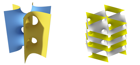
For the past two weeks we had the pleasure of working with Nicholas Sharp, Etienne Vouga, Josh Vekhter, and Erik Amezquita. We learned about a special type of minimal surfaces: triply-periodic minimal surfaces. Their name stems from their repeating pattern. Broadly speaking, a minimal surface minimizes its surface area. This is equivalent to having zero mean curvature. A triply-periodic minimal surface (TPMS) is a surface in \(\mathbb{R}^{3}\) that is invariant under a rank-3 lattice of translations.

Figure 1. (Left) A Minimal Surface [source] and (right) a TPMS [source].

Let’s talk about nonmanifold surfaces. “Manifold” is a geometry term that means: every local region of the surface looks like the plane (more formally — it is homeomorphic to a subset of Euclidean space). Non-manifold then allows for parts of the surface that do not look like the plane, such as T-junctions. Within the context of triangle meshes, a nonmanifold surface is a surface where more than 3 faces share an edge.

II. What We Did

First, we read and studied the 1993 paper by Pinkhall and Polthier that describes the algorithm for generating minimal surfaces. Our next goal was to generate minimal surfaces. Initially, we used pinned (Dirichlet) boundary conditions and regular manifold shapes. After ensuring that our code worked on manifold surfaces, we tested it on non-manifold input. 

Additionally, our team members learned how to use Blender. It has been a very enjoyable process, and the work was deeply satisfying, because of the embedded mathematical ideas intertwined with the artistic components. 

III. Reading the Pinkall Paper

“Computing Discrete Minimal Surfaces and Their Conjugates,” by Ulrich Pinkall and Konrad Polthier, is the classic paper on this subject; it introduces the iterative scheme we used to find minimal surfaces. Reading this paper was our first step in this project. The algorithm that finds a discrete locally area-minimizing surface is as follows:

  • Take the initial surface \(M_0\) with boundary \(∂M_0\) as first approximation of M. Set i to 0.
  • Compute the next surface \(M_i\) by solving the linear Dirichlet problem $$ \min_{M} \frac{1}{2}\int_{M_{i}}|\nabla (f:M_{i} \to M)|^{2}$$
  • Set i to i+1 and continue with step 2. 

The stopping condition is \(|\text{area}(M_i)-\text{area}(M_{i+1})|<\epsilon\). In our case, we used a maximum number of iterations, set by the user, as a stopping condition.

There are additional subtleties that must be considered (such as “what to do with degenerate triangles?”), but since we did not implement them — their discussion is beyond the scope of this post.

IV. Adding Periodic Boundary Conditions

This is, at its core, an optimization problem. To ensure that the optimization works, the boundary conditions have to be periodic instead of fixed in space. This is because we are enforcing a set of boundary conditions on periodic shapes — that is, tiling in a 3D space. 

IV(a). Matching Vertices

First, we need to check every two pairs of vertices in the mesh. We are looking  to see if they have identical coordinates in two dimensions, but are separated by exactly two units in the third dimension. When we find such pairs of vertices, we classify them to \(G_x\), \(G_y\), or \(G_z\). Note that we only store unique pairs.

IV(b). Laplacian Smoothness at the Boundary Vertices

Instead of using the discrete Laplacian, now we introduce a sparse matrix K to adjust our smoothness term based on the new boundary:

$$\min_{x}x^T(L^TK^TKL)x \text{ s.t. } x[b] = x_0[b].$$

Next, we construct the matrix K, which is a sparse square matrix of dimension #vertices by #vertices. To do so, we set \(K(i,i) = 1\), \(K(i,j) = 1\), and set the \(j\)th row entries to 0 for every pair of unique matched boundary vertices. For every interior vertex \(i\), we set \(K(i,i) = 1\).

IV(c). Aligning Boundary Vertices

Now we no longer want to pin boundary vertices to their original location in space. Instead, we want to allow our vertices to move, while the opposite sides of the boundary still match. To do that, we need to adjust the existing constraint term and to include additional linear constraints \(Ax=b\).

Therefore, we add two sets of linear constraints to our linear system:

  • For any pair of boundary vertices distanced by 2 units in one direction, the new coordinates should differ by 2 units.
  • For any pair of boundary vertices matched in the two other directions, the new coordinates should differ by 0.

We construct a selection matrix \(A\), which is a #pairs of boundary vertices in \(G\) by #vertices sparse matrix, to get the distance between any pair of boundary vertices. For every \(r\)th row, \(A(r,i)=1, A(r,j)=-1.\)$

Then we need to construct 3 \(b\) vectors, each of which is a sparse square matrix of the size [# of vector pairs of boundary vertices in G for a 3D coordinate (x,y,z)]. Based on whether at one given moment we are working with \(G_x\), \(G_y\), or \(G_z\), we enter \(2\) for those selected pairs, and \(0\) for the rest.

V. Correct Outcomes

Below, we can see the algorithm being correctly implemented. Each video represents a different mesh.

VI. Aesthetically Pleasing Bugs

Nothing is perfect, and coding in Matlab is no exception. We went through many iterations of our code before we got a functional version. Below are some examples of cool-looking bugs we encountered along the way, while testing the code on (what has become) one of our favorite shapes. Each video represents a different bug applied onto the same mesh.

VII. Conclusion and Future Work

Further work may include studying the physical properties of nonmanifold TPMS. It may also include additional basic structural simulations for physical properties, and establishing a comparison between the results for nonmanifold surfaces and the existing results for manifold surfaces.

Additional goals may be of computational or algebraic nature. For example, one can write scripts to generate many possible initial conditions, then use code to convert the surfaces with each of these conditions into minimal surfaces. An algebraic goal may be to enumerate all possible possibly-nonmanifold structures and perhaps categorize them based on their properties. This is, in fact, an open problem.

The possibilities are truly endless, and potential directions depend on the interests of the group of researchers undertaking this project further.

Categories
Geometry processing

Processing the Philosophy of Geometry

By Bryce Van Ross and Olga Guțan

Brief Existential Background 

Most branches of geometry are viewed as either (1) subsets of pure mathematics or (2) disciplines derived from problems in engineering, architecture, and computational mathematics. But what is geometry itself

Our work in the Summer Geometry Institute has been in the modern field of geometry processing. In this post, we will consider the philosophical aspects of geometry, and what they tell us about geometry processing specifically. The discussion has an inherent Eurocentric bias, and is, unfortunately, limited to Caucasian male philosophers.

The Roots of Geometry

In the eighteenth century, mathematics was primarily used to understand the natural sciences. For example, it was perceived as a language to better articulate physics, rather than as having intrinsic value. At that time, geometry was perceived as a form of applied mathematics. But where does the philosophy of geometry have its roots?

First we have Kant (1724-1804), who believed that our grasp of euclidean geometry must be instinctive. Opinions about this vary, based on each individual’s definitions of a priori knowledge and empiricism. Helmholtz, for example, agreed with Kant.

However, geometry processing incorporates not only euclidean geometry, but also calculus, linear algebra, differential equations, and topology. In addition, geometry processing includes a framework of algorithmic and optimization techniques. The knowledge of these topics varies from person to person, and therefore geometry processing can not be known a priori

Back to the 18th century: as logical empiricism became popular, the progress of philosophy of geometry stalled. Geometry was reduced to a system of definitions and conventions; logic and mathematics were given priority. As a result, the last big wave of interest in the philosophy of geometry was in the 1920s — 100 years ago, and 116 years after Kant!

Space as a Mathematical Concept

Mathematical conclusions depend on the structure we confer to a space. The structure determines the permissible elements, as well as the operations that can be applied to the elements. Without imposing structure, it is difficult to impose “rules,” and the potency of math is, thus, diluted. Most spaces in euclidean geometry exist; in fact, they are embedded in the reality we live in. With other kinds of geometry, we must define the properties of the space first. Then, we can ask: what are the conditions for creating a space? What kinds of spaces, and therefore geometries, can we have? (Our personal favorite is the geometry of chance.) 

Helmholtz (1821-1894) said the only allowable spaces are those that maintain constant curvature. This was eventually challenged by Einstein’s (1879-1955) Theory of Relativity. Weyl (1885-1955) came up with intuitive spaces, where it is possible to compare lengths only if two edges share the same spatio-temporal point. Similarly to the earlier-mentioned Kant (1724-1804), Carnap (1891-1970) claimed that intuition of spaces requires an n-dimensional topological space. As the philosophy of geometry evolved, so did our understanding of space.

“Waiting for Godot” in a Hyperbolic Space?

(The authors would like to gratefully acknowledge the primary source for the following sections.)

So what is geometry? Many people study it or use it… but what exactly are we interacting with?

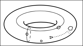
As an exercise of imagination, consider being a two-dimensional (2D) entity in a 2D universe. In fact, you don’t even have to imagine, somebody already wrote about this. The book is, unfortunately, at times misogynistic, but the geometry is intriguing to consider. Back to the exercise of imagination: since everything in the 2D universe is finite, is the universe itself finite? A 2D mathematician might suggest that the universe looks like a rectangle. Does, then, the universe have a point beyond which travel is impossible? If so, it likely is different from all other points of the universe, by its construction, since it has a boundary. Imagine you are playing Asteroids. As you move your rocket ship towards the right — once it reaches the boundary, it will reappear on the left side. In mathematical language we say that “the left edge of the rectangle has been identified, point by point, with the right edge.” 

Figure 1. A finite 2D world with no boundary. Source.

How to Build a Torus When You Are Two-Dimensional

In three dimensions, we can glue these boundaries. First, we bend the rectangle to produce a cylinder, while being careful to glue only the left and right edges together. Since we are operating in a ‘perfect’ thought-based mathematical world, the cylinder is malleable. Now we bend it to achieve this second gluing, which looks like a donut. We call this a torus.  

Figure 2. A torus. Source.

Recall that our reader currently lives in a 2D universe. A 2D person would not be able to see this torus in multiple dimensions. However, one would understand the space perfectly well, since the space can be identified back to the initial rectangle with edges. In this case, the universe is clearly finite, and with no edges.

Another surface with similar properties would be a two-dimensional sphere. A ladybug traveling on the sphere will notice that, locally, their world looks like a flat plane, and that the surface has no edges. On a small scale, if the mathematician ladybug splits the plane into triangles, the sum of the angles in each triangle will be 180 degrees. This is, in fact, known as a defining feature of euclidean geometry. However, on a larger scale, things start breaking.

A very large triangle drawn on the surface of the sphere has an angle sum far exceeding 180 degrees. Consider the triangle formed by the North Pole and two points on the equator of the sphere. The angle at each point on the equator is 90 degrees, so the total sum exceeds 180 degrees. Therefore, we conclude that — on a global scale — we can not apply euclidean geometry to a sphere. We call this hyperbolic geometry.

Figure 3. Angles add up to more than 180 degrees. Source.

Shape and Connection

To conclude this exercise of imagination, we must say that there is a wonderful connection between the shape (topology) of a surface and the type of geometry it inherits. This relationship is given, mathematically, by the Gauss-Bonnet equation:

\(\kappa A = 2 \pi \xi\)

Where \(\kappa \) is the Gaussian curvature of a surface, A is the element of area of the surface, \(\pi \) is our good old friend 3.1415…, and \(\xi\) is the Euler characteristic of the surface. In other words, the “geometry” is on the left side of the equation and the “topology” is on the right side of the equation; and the equal sign shows how deeply connected they are.

Studying various shapes and how they connect is not only interesting, but also important. Particularly, if a two-dimensional entity can deduce what sort of global geometry reigns their immediate world, they may be able to deduce the possible shapes for the things in their larger universe. 

To Really Conclude…

Although geometry processing has been around for a few decades, its philosophy is not yet well-studied. So far, this area shares themes with the broader philosophy of geometry, in certain topics:

  • a priori vs empiricist knowledge, 
  • the evaluation of space and its elements, 
  • geometric human intuition, 
  • construction of geometries, and 
  • the study of shape and connection. 

Given the computational aspect of geometry processing, there are additional important philosophical questions that arise, however they go beyond the scope of this post. It is difficult to determine whether such questions are best understood from the perspective of philosophy of geometry or philosophy of computer science, or both. 

As geometry processing continues to impact our technological world, the philosophy of geometry processing will grow too. In the meantime, we should continue critically questioning our programming, our modeling, and — most importantly — the ethical implications of our work. We must also ensure that we have a functional understanding of the parts that constitute geometry processing. At the same time, it must be said that the discipline is more than just the sum of its parts.

Categories
News

Reporting from the SGP Graduate School

SGI Fellows were registered for and invited to attend the Symposium on Geometry Processing (SGP), the premier venue for disseminating new research ideas and cutting-edge results in geometry processing.

I am writing this from the comfort of the EST time zone and from a boring but quiet dorm room. The Symposium on Geometry Processing (SGP) has successfully reminded me of the existence of a world outside my current location – a remarkable feat, especially given the forced geographic sedentarism of the past year and a half. Plenty of SGP attendees were active, participating, asking questions, and being engaged, despite it being late at night or very early in their time zones. Many other people will watch the SGP recordings on Youtube in the upcoming days. The concluding remark of “have a great day, or afternoon, or evening, depending on where you are right now” gave insight into precisely how geographically widespread the geometry processing community is.

Before delving further, some context is warranted: SGP is a yearly conference where people disseminate new results and ideas placed at the enticing intersection of theory and applications of mathematics, computer science, engineering, and other subjects. This year’s event is divided into the Graduate School (July 10-11) and the Conference (July 12-14). As I am writing this, it is July 11, so I have only attended the Graduate School events so far. 

Out of the talks I have attended, I want to focus on the Introduction to Geometry Processing Programing in MATLAB with gptoolbox. It is a fantastic tutorial prepared and presented by Hsueh-Ti Derek Liu, Silvia Sellán, and Oded Stein, and advised by Alec Jacobson. The tutorial is comprehensive and explains how things fit together in a bigger context. Furthermore, it provides the possibility for hands-on Matlab experience, which comes with solutions in case you get stuck.

For context, gptoolbox is a set of Matlab functions for geometry processing, aimed to make things easier and to prevent researchers from reinventing the wheel. I will tell you three new things I took away from the tutorial. This is, of course, not to say that there were only three things one could take away! In fact, I encourage you to watch the video and try to find more.

First, it was great to see how “from-the-ground-up” the teaching approach was. I prefer to prevent, rather than fix, technical crises, and the introductory bits of Matlab knowledge (such as: if you want to suppress the output of a statement, terminate the statement with a semicolon) were very welcome. I spent more evenings than I would like to admit trying to compile non-working code, only to realize – by trial-and-error – that my mistake was fixable in 3 seconds. As such, explicitly stating things, with no assumption of prior knowledge, was great.

My favorite part from Oded’s section was learning how to give objects shadows, as well as playing with the way light is reflected from the surface of the object. The tutorial covered techniques based on the Phong reflection model, so I look forward to learning additional approaches and more nuanced techniques.

Second, I was especially intrigued by the part on spectral conformal mapping in Derek’s section. Not only do we get to see the theoretical description of a geometric process, the knowledge of how important the subroutine is, and the paper it is first described in, but we also get a visual representation on how the algorithm works. We get a “before” and “after” picture of a shape that is familiar to us, alongside theoretical descriptions of mathematical objects. It turns out, you CAN have the best of both (mathematical) worlds!

Third, I was especially fascinated by the ability to triangulate a 2D shape in just two lines of code with the help of the get_pencil_curve function. The idea is that you can “call” the function and draw any shape you would like, using your mouse click as the line input. First, Silvia illustrated the need for such a tool before introducing it. But also, after triangulating the figure, she outlined – for comparison – the work one might need to do to get the same result had we not had gptoolbox. The alternative included at least two other programs and the word “export” multiple times, which not only sounds like a lot of work, but also like a logistical nightmare.

As a newcomer to geometry processing, it was good to see the dedication to knowledge exchange and the great efforts made to be inclusive towards the largest possible number of people. I spent part of this summer watching geometry processing courses to bring myself up to speed with the discipline, and my brain was ecstatic when it recognized concepts I had studied earlier, or when it was able to make connections on its own. The existence of the Graduate School made me only more excited for what is in store for the rest of the conference and for the rest of the summer. So, I am keeping my brain open for all the knowledge acquisition that will undoubtedly occur during SGP and, afterwards, during Summer Geometry Institute (SGI).

Lastly – the Graduate School at SGP gave me an idea of the level of growth I will experience in the coming weeks, first at the SGP talks, and – next – at SGI. Not only will I learn a lot, but it will also be fun and incredibly rewarding! I think it will be especially interesting to put this post side by side with one I will write closer to the end of the SGI program, and to compare the difference marked by a few weeks of intensive learning.