Deep Learning – SGI 2021

By Faria Huq, Kinjal Parikh, Lucas Valença

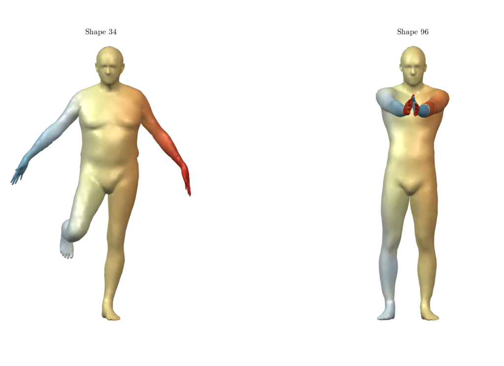
During the 4^th week of SGI, we worked closely with Dr. Tal Shnitzer to develop an improved loss function for learning functional maps with robustness to symmetric ambiguity. Our project goal was to modify recent weakly-supervised works that generated deep functional maps to make them handle symmetric correspondences better.

Introduction:

Shape correspondence is a task that has various applications in geometry processing, computer graphics, and computer vision – quad mesh transfer, shape interpolation, and object recognition, to name a few. It entails computing a mapping between two objects in a geometric dataset. Several techniques for computing shape correspondence exist – functional maps is one of them.

A functional map is a representation that can map between functions on two shapes’ using their eigenbases or features (or both). Formally, it is the solution to \(\mathrm{arg}\min_{C_{12}}\left\Vert C_{12}F_1-F_2\right\Vert^2\), where \(C_{12}\) is the functional map from shape \(1\) to shape \(2\) and \(F_1\), \(F_2\) are corresponding functions projected onto the eigenbases of the two shapes, respectively.

Therefore, there is no direct mapping between vertices in a functional map. This concise representation facilitates manipulation and enables efficient inference.

Figure 1: The approach proposed by Sharma and Ovsjanikov may fail on symmetric regions. Notice the hands, which have not been matched correctly due to their symmetric structure.

Recently, unsupervised deep learning methods have been developed for learning functional maps. One of the main challenges in such shape correspondence tasks is learning a map that differentiates between shape regions that are similar (due to symmetry). We worked on tackling this challenge.

Background

We build upon the state-of-the-art work “Weakly Supervised Deep Functional Map for Shape Matching” by Sharma and Ovsjanikov, which learns shape descriptors from raw 3D data using a PointNet++ architecture. The network’s loss function is based on regularization terms that enforce bijectivity, orthogonality, and Laplacian commutativity.

This method is weakly supervised because the input shapes must be equally aligned, i.e., share the same 6DOF pose. This weak supervision is required because PointNet-like feature extractors cannot distinguish between left and right unless the shapes share the same pose.

To mitigate the same-pose requirement, we explored adding another component to the loss function Contextual Loss by Mechrez et al. Contextual Loss is high when the network learns a large number of similar features. Otherwise, it is low. This characteristic promotes the learning of global features and can, therefore, work on non-aligned data.

Work

Model architecture overview: As stated above, our basic model architecture is similar to “Weakly Supervised Deep Functional Map for Shape Matching” by Sharma and Ovsjanikov. We use the basic PointNet++ architecture and pass its output through a \(4\)-layer ResNet model. We use the output from ResNet as shape features to compute the functional map. We randomly select \(4000\) vertices and pass them as input to our PointNet++ architecture.
Data augmentation: We randomly rotated the shapes of the input dataset around the “up” axis (in our case, the \(y\) coordinate). Our motivation for introducing data augmentation is to make the learning more robust and less dependent on the data orientation.
Contextual loss: We explored two ways of adding contextual loss as a component:
1. Self-similarity: Consider a pair of input shapes (\(S_1\), \(S_2\)) of features \(P_1\) with \(P_2\) respectively. We compute our loss function as follows:
  \(L_{CX}(S_1, S_2) = -log(CX(P_1, P_1)) – log(CX(P_2, P_2))\),
  where \(CX(x, y)\) is the contextual similarity between every element of \(x\) and every element of \(y\), considering the context of all features in \(y\).
  More intuitively, the contextual loss is applied on each shape feature with itself (\(P_1\) with \(P_1\) and \(P_2\) with \(P_2\)), thus giving us a measure of ‘self-similarity’ in a weakly-supervised way. This measure will help the network learn unique and better descriptors for each shape, thus alleviating errors from symmetric ambiguities.
2. Projected features: We also explored another method for employing the contextual loss. First, we project the basis \(B_1\) of \(S_1\) onto \(S_2\), so that \(B_{12} = B_ 1 \cdot C_{12}\). Similarly, \(B_{21} = B_2 \cdot C_{21}\). Note that the initial bases \(B_1\) and \(B_2\) are computed directly from the input shapes. Next, we want the projection \(B_{12}\) to get closer to \(B_2\) (the same applies for \(B_{21}\) and \(B_1\)). Hence, our loss function becomes:
  \(L_{CX}(S_1, S_2) = -log(CX(B_{21}, B_1)) – log(CX(B_{12}, B_2))\).
  Our motivation for applying this loss function is to reduce symmetry error by encouraging our model to map the eigenbases using \(C_{12}\) and \(C_{21}\) more accurately.
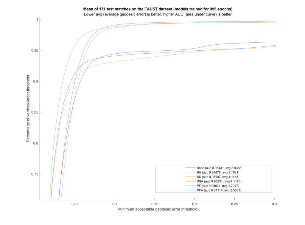
Geodesic error: For evaluating our work, we use the metric of average geodesic error between the vertex-pair mappings predicted by our models and the ground truth vertex-pair indices provided with the dataset.

Result

We trained six different models on the FAUST dataset (which contains \(10\) human shapes at the same \(10\) poses each). Our training set includes \(81\) samples, leaving out one full shape (all of its \(10\) poses) and one full pose (so the network never sees any shape doing that pose). These remaining \(19\) inputs are the test set. Additionally, during testing we used ZoomOut by Melzi et al.

Model	Data Augmentation	Contextual Loss
Base	False	None
BA	True	None
SS	False	Self Similarity
SSA	True	Self Similarity
PF	False	Projected Features
PFA	True	Projected Features

Table 1: We trained 7 models using the settings described in this table

Figure 2: The AUC (area under curve) curves and values with the average geodesic error for each model.

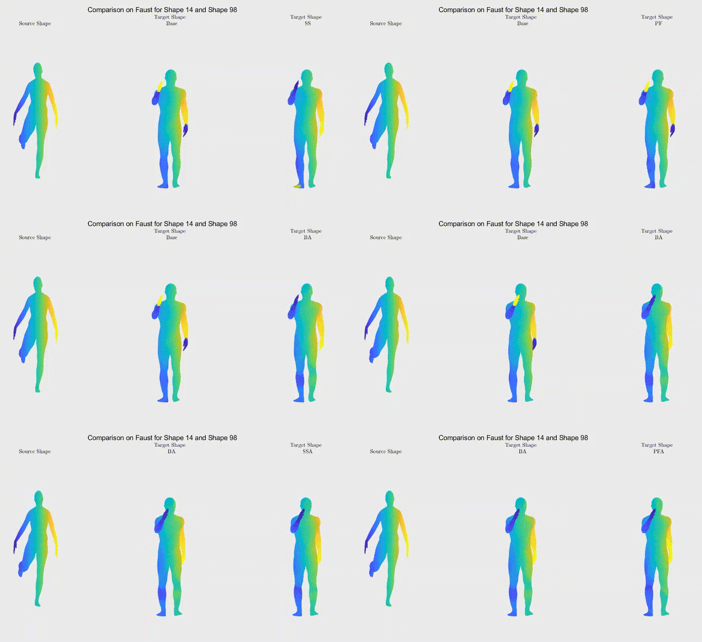
For qualitative comparison purposes, the following GIF displays a mapping result. Overall, the main noticeable visual differences between our work and the one we based ourselves on appeared when dealing with symmetric body parts (e.g., hands and feet).

Figure 3: Comparison between shape correspondence produced by the models described in Table 1.

Still, as it can be seen, the symmetric body parts remain the less accurate mappings in our work too, meaning there’s still much to improve.

Conclusion

We thoroughly enjoyed working on this project during SGI and are looking forward to investigating this problem further, to which end we will continue to work on this project after the program. We want to extend our deepest gratitude to our mentor, Dr. Tal Shnitzer, for her continuous guidance and patience. None of this would be possible without her.

Thank you for taking the time to read this post. If there are any questions or suggestions, we’re eager to hear them!