Categories
research

Surface Reconstruction with Topological Data Analysis

This blog post was inspired by the talk given by Prof. Yusu Wang during SGI. We use Topological Data Analysis to showcase its feature characterization principles and how it can be used for point cloud surface reconstruction. The code used to generate the different results below are stored on SGI’s GitHub, so give it a try. Let’s go!

Brief Introduction into Persistent Homology

Persistent homology is formed of two words: persistent and homology. Homology comes from homology groups, an intersection between group theory and topology. On a high-level, two objects are homotopic if they can be continuously deformed into one another. As such, they belong to the same group or class because they share the same properties. These homotopy properties can be commonly referred to in examples as the number of holes that an object possesses.

Homology is then used to describe more complex objects such as Simplicial Complexes and Functions.

If we take functions, we can map every set level to a property that describes this function. This can best be seen as features induced by local extrema. Local minima tell us that a new feature was born (similar to the hole concept) and the local maxima tell us that some features have been merged and as a result no longer exist. The function below showcases two minima, which means two features are alive at some point simultaneously and disjointly (two separate holes filled water), but will disappear and be merged once the level-set reaches the local maximum.
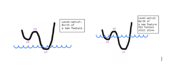
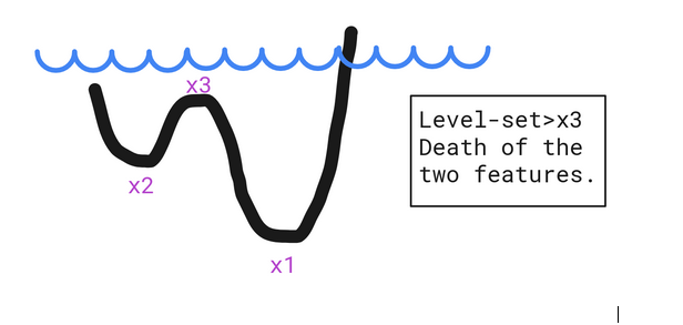
Features can be seen as local minima that are covered with a level-set.
The death of the features happens when they get merged at a local maximum.

For a set of points, the characterization happens by first constructing a Simplicial Complex (Vietoris-Rips Complex, Čech Complex,…). This follows a logic which connects the points whose circles with radius r centered around them intersect. This is how k-simplices (such as points, edges,triangles, etc. where k is the number of mutually intersecting circles) are built. What happens afterwards is that, in order to find the characteristics of a set of points, the radius r is increased and as we go, the features are detected from the resulting Simplicial Complex.
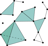
Simplicial Complex.
Source: https://en.wikipedia.org/wiki/Simplicial_complex

Now that we have our features, we need to measure their importance and this is what persistence is meant to do. Persistence, is then the act of quantifying the difference between the death and birth of these features, i.e how long a specific feature existed. which helps in assessing the importance of a feature.

For this reason, Persistent Homology can serve as a de-noising tool or can simply act as an object descriptor.

GUDHI: Library for Topological Data Analysis (TDA)

Now, let’s see all of the concepts we have explained in practice. For that, we will use the GUDHI library for Topological Data Analysis.

We present the following examples to showcase the persistence diagrams obtained for different set of points.

Persistence diagrams have these properties: 1) The red points are the 0-simplices, which are dots, points or disks. 2) The blue points are the 1-simplices characterized by a hole. 3) The points that are far off the diagonal live longer, which means that they are more prominent/important.

For the first example, we can see for instance that one blue dot is very far from the diagonal, which means that this is one of the most important features of our set. The other blue dots which stem from the gap between our points but disappear quickly.
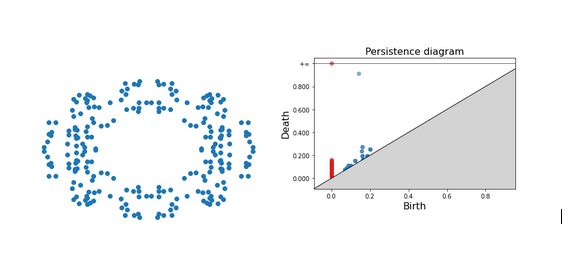
Persistence Diagram of a set of points forming a ring.

For the second example, we present two persistence diagrams based on two maximum radius thresholds. For a small threshold, we only have one blue dot; the smaller ring is detected because a small threshold matches its small radius. As this threshold gets bigger, we are then able to detect the second bigger ring. Increasing the threshold even further merges these two circles into one component as the different vertices get connected in an indiscernible way.
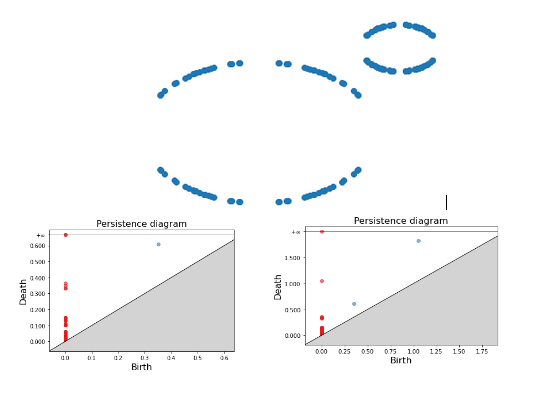
1) (Left) Persistence Diagram of a set of points forming two rings with a small maximum threshold.
2) (Right) Persistence Diagram of a set of points forming two rings with a big maximum threshold.

Surface Reconstruction with TDA

Now that we have used the different elements from the Topological Data Analysis, we will adopt the Simplicial Complex concept and use it to create the surface of a known mesh: spot.
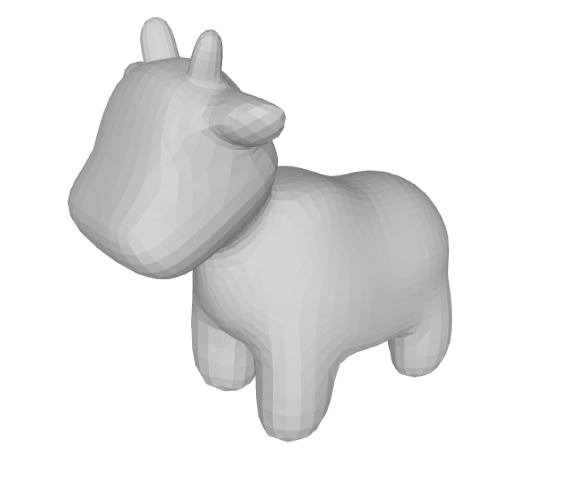
The original mesh.

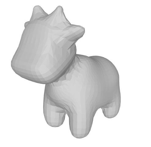
We only consider the point cloud from the mesh and try to estimate the surface by creating the connections between three vertices at once. Once these connections are made, we save a new mesh with these faces connections. Depending on the threshold set to connect the vertices we obtain different levels of precision:
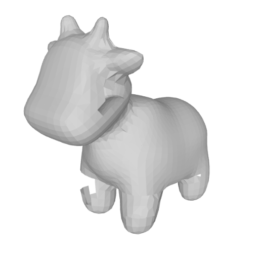
Reconstruction based on the faces from Vietoris-Rips Complex with a low maximum threshold.
Reconstruction based on the faces from Vietoris-Rips Complex with a big maximum threshold.

Conclusion

We have shown in this blog post how Topological Data Analysis and in particular Persistent Homology can be used to find structure in a set of points. This can lead to characterizing the set’s properties in addition to allowing the execution of known tasks in Geometry Processing such as Surface Reconstruction.

References

[1] Persistent Homology—a Survey, Herbert Edelsbrunner and John Harer.

[2] https://en.wikipedia.org/wiki/Homology_(mathematics)

[3] GUDHI, https://gudhi.inria.fr/
Categories
tutorial week

Redesigning the Playing Cards

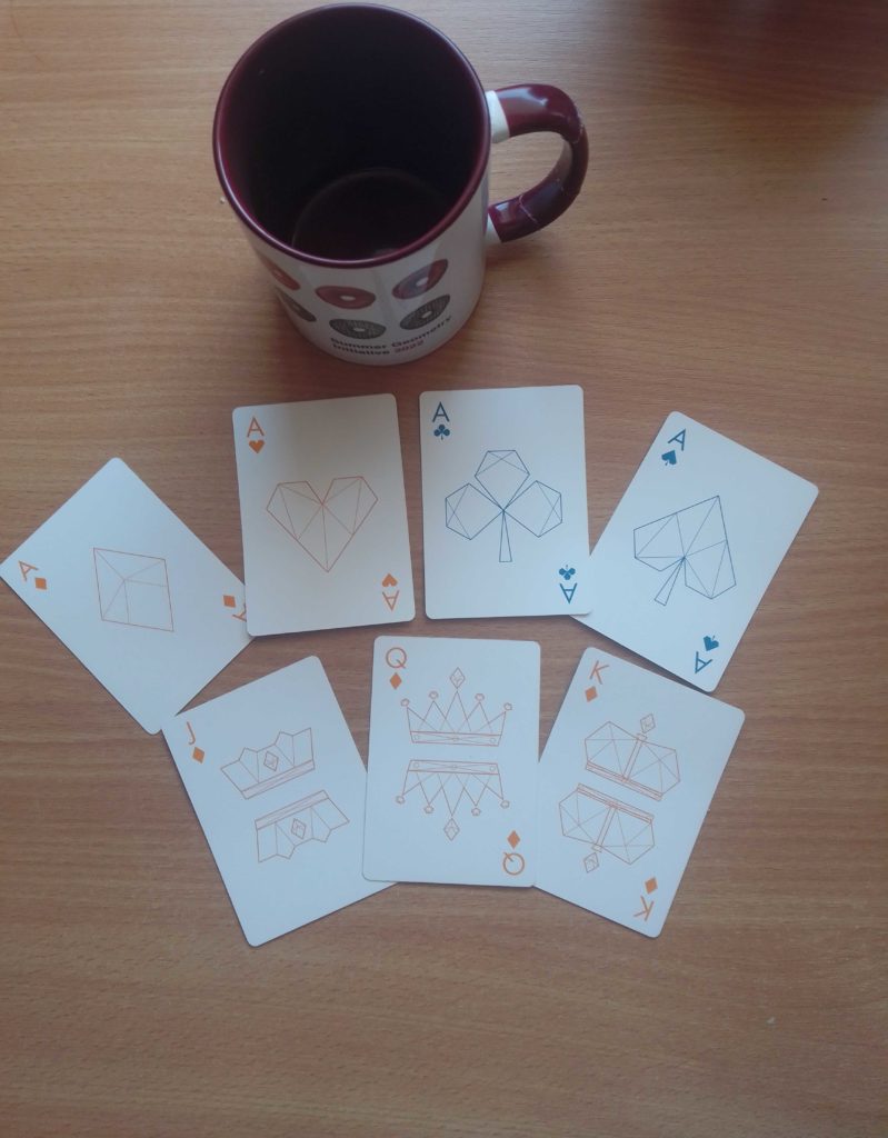
Selection of Cards from MathWorks’ Playing Cards…. and the SGI 2022 Mug.

For my first SGI blog, I have decided to combine what we have learned during the second day of the tutorial week given by the amazing Silvia Sellán to get an alternative version of the playing cards that we, fellows, have received in the swag package. The code can be found on SGI’s GitHub.

The cards are nicely designed already, so the goal is not to get a superior design but to put the knowledge we have collected into practice.

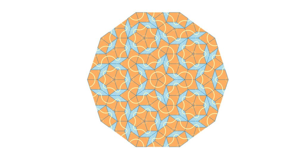
If you are curious about how the design was made by Mathworks, you can consult this website where they provide an explanation of the code that went into building the patterns. To briefly summarize the concept, the patterns were made using a Penrose Tiling, an aperiodic tiling that covers a surface with shapes such as triangles, polygons, etc. The Penrose Tiling is more distinct in larger surfaces where the tile’s repetition creates a distinct pattern.

Penrose tiling as obtained after running the steps in the Playing Cards blog.

The tiling in the deck of playing cards is much simpler than what the Penrose Tiling usually ends up looking like because the number of tiles used to divide the shapes is very small. The aim is to recreate a simple pattern using triangulation principles that we have covered during the tutorial week.

The steps making our approach, which we are going to detail in this post, can be summarized in the pipeline below:

Pipeline

The idea used to recreate the cards is based on two commands, one of them being the drawing tool from the gpltoolbox and the triangulation tool:

[V,E,cid] = get_pencil_curves(1e-6); (1)

[U,G] = triangle(V,E,[],'Flags','-q30'); (2)

To recreate the style of the playing cards, we will need to transfer the drawing obtained in (1) to a polyline-based design. The drawing from get_pencil_curve is never straight, so we have to detect the existing segments and estimate their positions.

To achieve this polyline-based design, the position of the segment bounds and their connections are estimated which means that to recreate the polylines, we need to estimate the points that have corner properties and build the connections between these points.

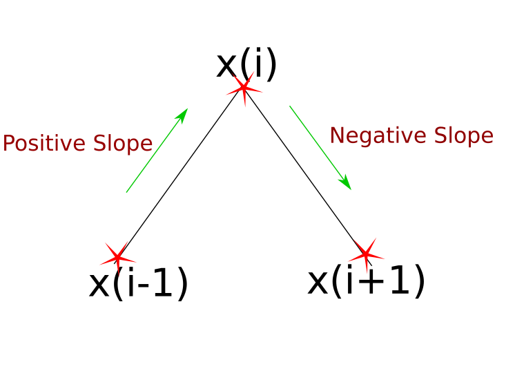
To execute the step that consists of detecting these corner points, we can use the script find_corners.m. The principle is simple: a corner point is a point \(x_{i}\) where the sign of the derivative changes when measured between \(x_{i}\)’s predecessor \(x_{i-1}\) and successor \(x_{i+1}\). The edge cases where vertical lines exist in the drawing and that yield to +/-Inf derivatives and the case of horizontal lines that have a zero derivative along the segment are also accounted for.

\(x_{i}\) is a corner with a change in the slope’s sign.

Points that satisfy this change in the slope’s sign will be considered corner candidates. At the end of the corner detection process, a pruning occurs to discard points that are very close to each other. Once we have these corner points, the polylines can be immediately seen as the connection between two consecutive corners.

Curvatures also naturally trigger this change in the slope’s sign. We do however need to distinguish between an intentional curvature and a non-intentional one caused by drawings which inherently have lines with varying degrees of curvature attributed to hand made drawings with the get_pencil_curve tool. This is solved by fixing a derivative threshold that discards very small variations.

When the polyline-based design is ready, we can run the triangulation tool as in (2) to obtain our resulting shapes.

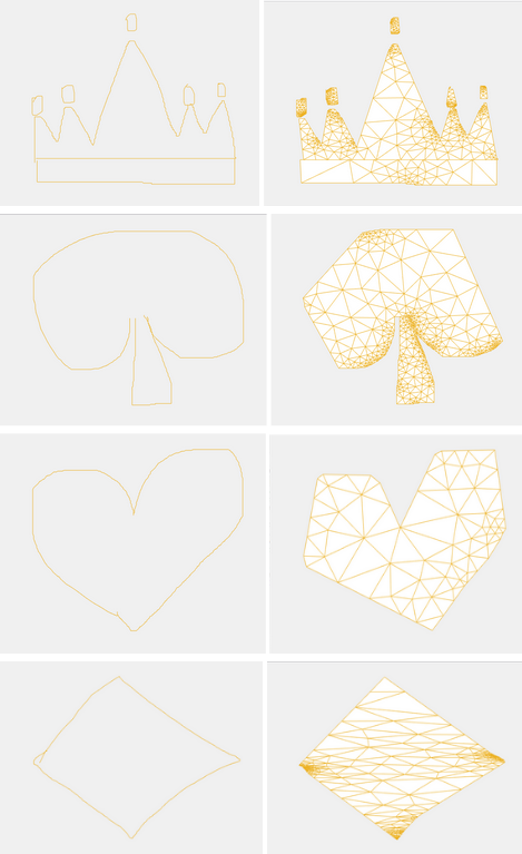
In the pictures below, we have collected the results from our algorithm which generated triangulated polyline versions of shapes created by users. The results are not perfect due to many irregularities in the original drawing. These irregularities stem from the low quality of the drawings when using a mouse instead of an actual pen.

A queen, a spade, a heart and a diamond before and after triangulation.

Some interesting observations can be made from the results of the heart and spade shapes: the algorithm converts their curved lines into two straight lines which meet at a point that showcases corner properties which validates that strong curvatures are properly considered and the inevitable ones are discarded.

And with that, we can finally say that we have our own “artsy” playing cards design or maybe this could already be Mathworks’ design in a parallel universe!