By Caroline Huber, Alan Goldfarb, and Denisse Garnica
In the first project of SGI, for us, Julia Sets – where we (in simple terms) attempt to approximate 2D and 3D shapes with a Julia Set – much interesting work was done. The official problem statement is: Can we train a neural network to predict the corresponding filled Julia set approximation for any given input shape? With daily collaborative meetings and independent coding work we first attempted to understand how to construct these sets with code. We worked our way through several established papers on the subject both independently as well as in several collaborative zooms (see pdfs below).


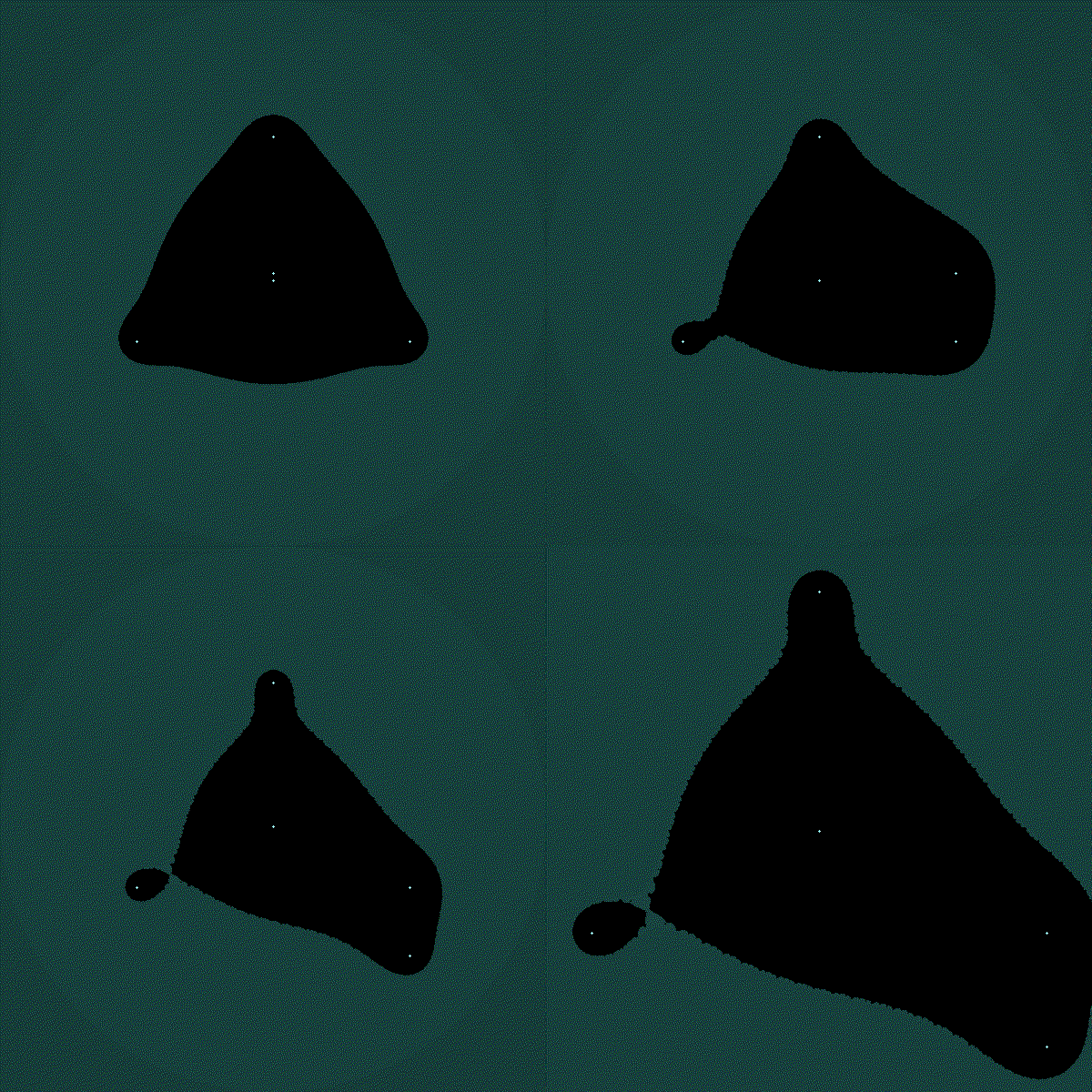
Then, we worked on experimenting with some base code that one of our mentors, Richard Liu, provided. By experimenting, we mean that we altered various attributes of the presented function and observed the effects on the fractal output. We changed the values of the roots, their multiplicities, the number of roots, and we added scalar multiples and so on. For reference, Figure 1 is the original fractal. Multiplying by a scalar less than one resulted in less separation between the affected roots (closer together). This is shown in the following figures: multiplying the whole function by a scalar of 0.5 resulted in figure 2 and multiplying just the second and fourth roots by a scalar multiple of 0.5 resulted in figure 3.


Conversely, multiplying by a scalar larger than 1 resulted in increased separation between the affected roots (farther apart). The result of multiplying by a scalar of 1.3 resulted in figure 4.


Further experimentation included scalar multiple and changing all roots to be double (multiplicity 2), as seen in figure 5, and scalar multiple with only changing the multiplicity of a single root (to be double), as seen in figure 6.
We created a function to add color to the non-Julia Set points. Defining the color with the “escape velocity”. The Julia set -explained in a very ambiguous way- is a set of points that stays in some certain region after many iterations of a function. The “escape velocity” is how long it takes to a point to go outside the region. According to that number we change the color of the point. And we obtain images like this one.

Here all the black points represent the Julia set. The dark-green points are the ones that have a minor escape velocity and the brightest are the ones that took longer to go outside.
We decided that it would be helpful to be able to zoom into these fractals and see what they look like up close (especially with the alterations). So, we added code that zoomed in on a point slightly off-center. Then, we combined several of those images into a gif that runs through them all. (see attachment 1)

We collaborated to create another gif that runs through frames where the root location is altered, and the picture zooms in on this change. We provided the code to identify and alter the roots and then combined the frames. (see attachment 2 for altered root multiplicities and attachment 3 for a zoom of altered roots).


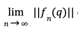
Now that Julia sets have been seen in an intuitive way, let’s see a little more formality. Julia sets of rational maps are determined as follows: Given a rational map (a function of the form f(q)) a complex number q is in the corresponding Julia set if the below limit does not diverge. Here, fn denotes the nth recursion of f. The constants r1,r2, . . ., rt and s1, s2 , . . .,sb are respectively called the top and bottom roots of f.


In order to generate plots of these sets we approximated the set by iterating the function a fixed number of times and comparing the output against a threshold value. Only inputs which produced a value below the threshold were included in the Julia set. We then plotted the filled Julia set by plotting the interior of the Julia set.
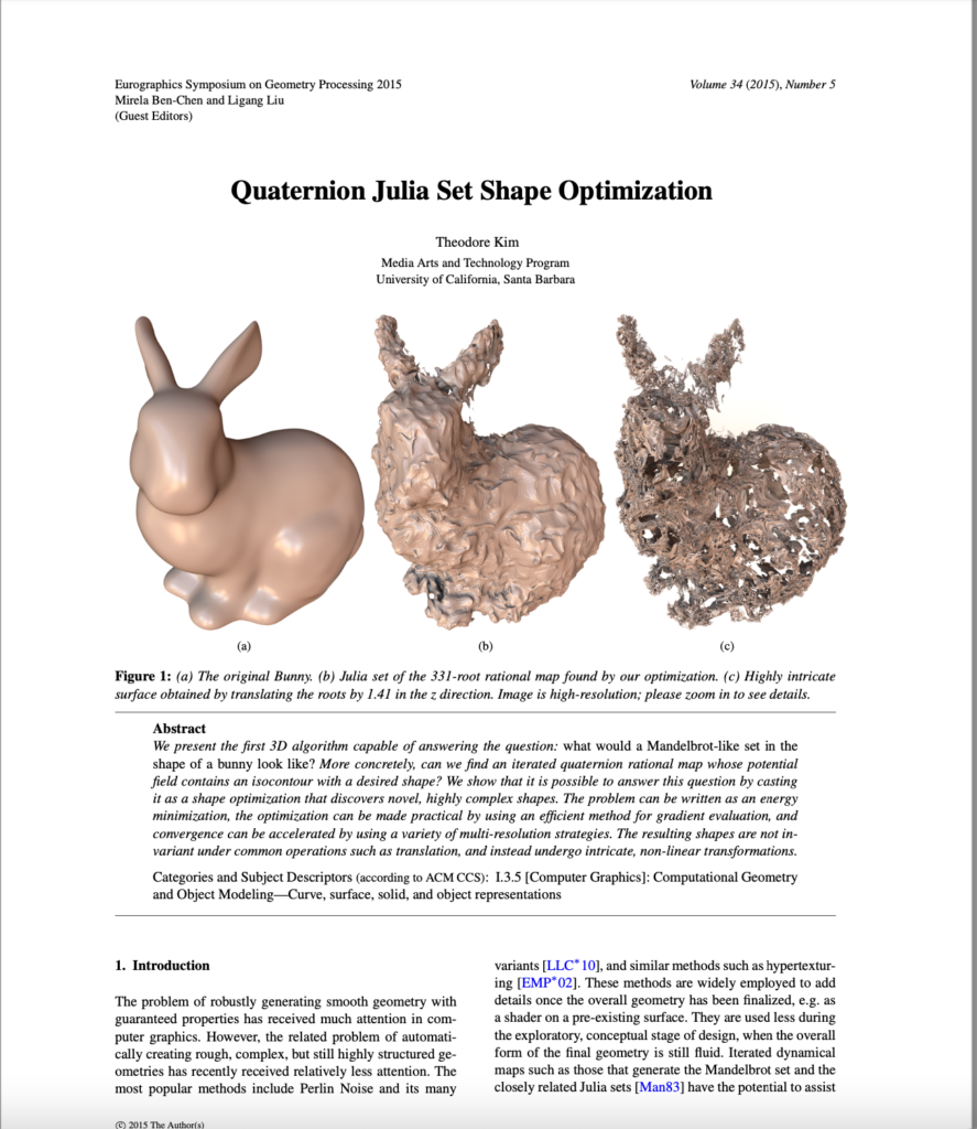
Some of the filled Julia sets we generated behaved in ways which differed from our initial expectations. According to a paper by Dr. Theodore Kim, points close enough to top roots would be included in the filled Julia set and points close enough to bottom roots would not. Dr. Kim stated that to approximate a given curve with a Julia set one should use a rational function with roots along that curve. However, we realized that symmetric placement of the roots can generate asymmetric Julia sets and that placing roots along the boundary of a shape did not always produce a filled Julia set corresponding to that shape.
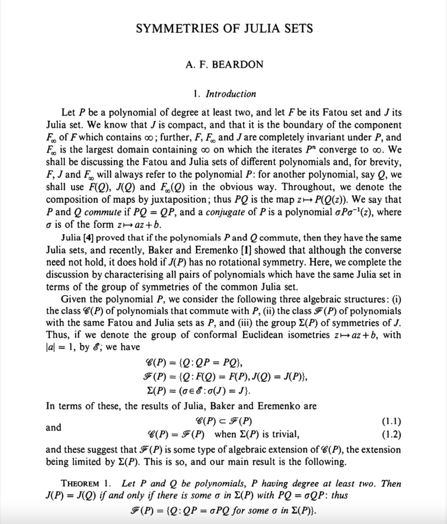
In order to get a better understanding of why this might be occurring, we read a few papers describing the mathematical structure of Julia sets of rational functions. We delved deeper into these papers and explained some strange properties about Julia sets. For instance, a Julia set of a polynomial cannot have any mirror symmetries which are not also rotational symmetries. This is the case even if the placement of the roots is symmetric. This led us to the realization that adding roots to a function can have global consequences on the shape of the function’s Julia set which makes the problem of approximating even simple shapes with Julia sets seem more difficult than initially anticipated.
This project has been very interesting for the three of us and we are looking forward to see what we can achieve in the future. We will continue exploring Julia sets, and hopefully we will be able to approximate interesting figures!