Categories
Math

The Area of a Circle

Author: Ehsan Shams (Alexandria University, Egypt)

“Since people have tried to prove obvious propositions,
they have discovered that many of them are false.”
Bertrand Russell

Archimedes proposed an elegant argument indicating that the area of a circle (disk) of radius \(r\) is \( \pi r^2 \). This argument has gained attention recently and is often presented as a “proof” of the formula. But is it truly a proof?

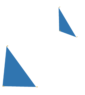
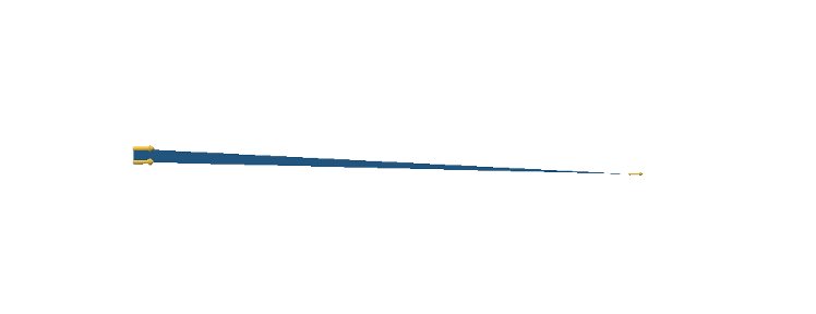
The argument is as follows: Divide the circle into \(2^n\) congruent wedges, and re-arrange them into a strip, for any \( n\) the total sum of the wedges (the area of the strip) is equal to the area of the circle. The top and bottom have arc length \( \pi r \). In the limit the strip becomes a rectangle, meaning as \( n \to \infty \), the wavy strip becomes a rectangle. This rectangle has area \( \pi r^2 \), so the area of the circle is also \( \pi r^2 \).

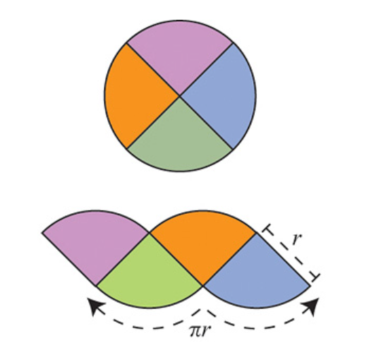
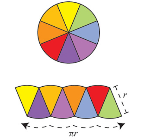
These images are taken from [1].

To consider this argument a proof, several things need to be shown:

  1. The circle can be evenly divided into such wedges.
  2. The number \( \pi \) is well-defined.
  3. The notion of “area” of this specific subset of \( \mathbb{R}^2 \) -the circle – is well-defined, and it has this “subdivision” property used in the argument. This is not trivial at all; a whole field of mathematics called “Measure Theory” was founded in the early twentieth century to provide a formal framework for defining and understanding the concept of areas/volumes, their conditions for existence, their properties, and their generalizations in abstract spaces.
  4. The limiting operations must be made precise.
  5. The notion of area and arc length is preserved under the limiting operations of 4.

Archimedes’ elegant argument can be rigorised but, it will take some of work and a very long sheet of paper to do so.

Just to provide some insight into the difficulty of making satisfactory precise sense of seemingly obvious and simple-to-grasp geometric notions and intuitive operations which are sometimes taken for granted, let us briefly inspect each element from the above.

Defining \( \pi \):

In school, we were taught that the definition of \( \pi \) is the ratio of the circumference of a circle to its diameter. For this definition to be valid, it must be shown that the ratio is always the same for all circles, which is
not immediately obvious; in fact, this does not hold in Non-Euclidean geometry.

A tighter definition goes like this: the number \( \pi \) is the circumference of a circle of diameter 1. Yet, this still leaves some ambiguity because terms like “circumference,” “diameter,” and “circle” need clear definitions, so here is a more precise version: the number \( \pi \) is half the circumference of the circle \( \{ (x,y) | x^2 + y^2 =1 \} \subseteq \mathbb{R}^2 \). This definition is clearer, but it still assumes we understand what “circumference” means.

From calculus, we know that the circumference of a circle can be defined as a special case of arc length. Arc length itself is defined as the supremum of a set of sums, and in nice cases, it can be exactly computed using definite integrals. Despite this, it is not immediately clear that a circle has a finite circumference.

Another limiting ancient argument that is used to estimate and define the circumference of a circle and hence calculating terms of \( \pi \) to some desired accuracy since Archimedes was by using inscribed and circumscribed regular polygons. But still, making a precise sense of the circumference of a circle, and hence the number \( \pi \), is a quite subtle matter.

The Limiting Operation:

In Archimedes’ argument, the limiting operation can be formalized by regarding the bottom of the wavy strip (curve) as the graph of a function \(f_n \), and the limiting curve as the graph of a constant function \(f\). Then \( f_n \to f \) uniformly.

The Notion of Area:

The whole of Euclidean Geometry deals with the notions of “areas” and “volumes” for arbitrary objects in \( \mathbb{R}^2 \) and \( \mathbb{R}^3 \) as if they are inherently defined for such objects and merely need to be calculated. The calculation was done by simply cutting the object into finite simple parts and then rearranging them by performing some rigid motion like rotation or translation and then reassembling those parts to form a simpler body which we already know how to compute. This type of Geometry relies on three hidden assumptions:

  • Every object has a well-defined area or volume.
  • The area or volume of the whole is equal to the sum of the areas or volumes of its parts.
  • The area or volume is preserved under such re-arrangments.

This is not automatically true for arbitrary objects; for example consider the Banach-Tarski Paradox. Therefore, proving the existence of a well-defined notion of area for the specific subset describing the circle, and that it is preserved under the subdivision, rearrangement, and the limiting operation considered, is crucial for validating Archimedes’ argument as a full proof of the area formula. Measure Theory addresses these issues by providing a rigorous framework for defining and understanding areas and volumes. Thus, showing 1,3, 4, and the preservation of the area under the limiting operation requires some effort but is achievable through Measure Theory.

Arc Length under Uniform Limits:

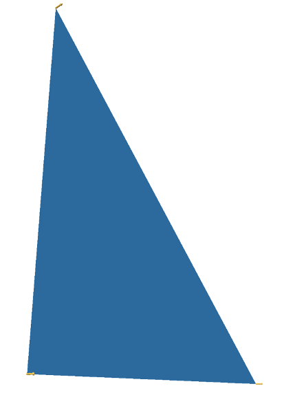
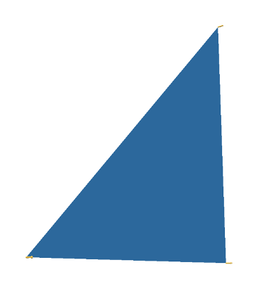
The other part of number 5 is slightly tricky because the arc length is not generally preserved under uniform limits. To illustrate this, consider the staircase curve approximation of the diagonal of a unit square in \( \mathbb{R}^2 \). Even though as the step curves of the staircase get finer and they converge uniformly to the diagonal, their total arc length converges to 2, not to \( \sqrt{2} \). This example demonstrates that arc length, as a function, is not continuous with respect to uniform convergence. However, arc length is preserved under uniform limits if the derivatives of the functions converge uniformly as well. In such cases, uniform convergence of derivatives ensures that the arc length is also preserved in the limit. Is this provable in Archimedes argument? yes with some work.

Moral of the Story:

There is no “obvious” in mathematics. It is important to prove mathematical statements using strict logical arguments from agreed-upon axioms without hidden assumptions, no matter how “intuitively obvious” they seem to us.

“The kind of knowledge which is supported only by
observations and is not yet proved must be carefully
distinguished from the truth; it is gained by induction, as
we usually say. Yet we have seen cases in which mere
induction led to error. Therefore, we should take great
care not to accept as true such properties of the numbers
which we have discovered by observation and which are
supported by induction alone. Indeed, we should use such
a discovery as an opportunity to investigate more exactly
the properties discovered and to prove or disprove them;
in both cases we may learn something useful.”
L. Euler

“Being a mathematician means that you don’t take ‘obvious’
things for granted but try to reason. Very often you will be
surprised that the most obvious answer is actually wrong.”
–Evgeny Evgenievich

Bibliography

  1. Strogatz, S. (1270414824). Take It to the Limit. Opinionator. https://archive.nytimes.com/opinionator.blogs.nytimes.com/2010/04/04/take-it-to-the-limit/
  2. Tao, T. (2011). An introduction to measure theory. Graduate Studies in Mathematics. https://doi.org/10.1090/gsm/126
  3. Pogorelov, A. (1987). Geometry. MIR Publishers.
  4. Blackadar, B. (2020). Real Analysis Notes
Categories
Research

Fitting Surfaces with Noise Regularization

Mentor: Amir Vaxman

Volunteer: Alberto Tono

Fellows: Mutiraj Laksanawisit, Diana Aldana Moreno, Anthony Hong

Our task is to fit closed and watertight surfaces to point clouds that might have a lot of noise and inconsistent outliers. There are many papers like this, where we will explore a modest variation on the problem: we will allow the system to modify the input point clouds in a controlled manner, where the modification will be gradually scaled back until the method fits to the original point clouds. The point of this experiment is to check whether such modification is beneficial for both accuracy and training time.

Regular Point-Cloud Fitting

A point clouds is an unordered set of 3D points: \(\mathscr{P}=\left\{x_i, y_i, z_i\right\}\), where \(0<i\leq N\) for some size \(N\). These points can be assumed to be accompanied by normals \(n_i\) (as unit vectors associated to each points). An \emph{implicit} surface reconstruction tries to fit a function \(f(x,y,z)\) to every point in space, such that its zero set
$$
S = f^{-1}(0)=\left\{(x,y,z) | f(x,y,z)=0\right\}
$$
represents the surface.

We usually train \(f\) to be a signed distance function (SDF) \(\mathbb{R}^3\rightarrow\mathbb{R}\) from the zero set. That is, to minimize the loss:
$$
f = \text{argmin}\left(\lambda_{p}E_p+\lambda_{n}E_n+\lambda_{s}E_s\right)
$$

where
\begin{align}
E_p &= \sum_{i=0}^N{|f(x_i,y_i,z_i)|^2}\\
E_n &= \sum_{i=0}^N{|\nabla f(x_i,y_i,z_i)-n_i|^2}\\
E_s &= \sum_{j=0}^Q{||\nabla f(x_j,y_j,z_j)|-1|^2}
\end{align}
Loss term \(E_p\) is for the zero-set fitting. Loss term \(E_n\) is for the normal fitting, and term \(E_s\) is for regulating \(f\) to be an SDF; it is trained on a randomly sampled set \(\mathscr{Q}=\left(x_j,y_j,z_j\right)\) (of size \(Q=|\mathscr{Q}|\)) in the bounding box of the object, that gets replaced every few iterations. The bounding box should be a bit bigger, say cover %20 more in each axis, to allow for enough empty space around the object.

Reconstruction Results

We extracted meshes from this repository and apply Poisson disc sampling with point-number parameter set at 1000 (but note that the resulted sampled points are not 1000; see the table below) on MeshLab2023.12. We then standardize the grids and normalize the normals (the xyz file with normals does not give normals in this version of MeshLab so we need to an extra step of normalization). Then we ran the learning procedure on these point clouds to fit an sdf with 500 epochs and other parameters shown below.

net = train_sdf_net(standardized_points, normals, epochs=500, batch_size=N,
learning_rate=0.01, lambda_p=1.0, lambda_n=1.5, lambda_s=0, neuron_factor=4)

We then plots the results (the neural netwok, the poitclouds and normals) and registered isosurfaces as meshes on polyscope and used slice planes to see how good are the fits. Check the table below.

NefertitiHomerKitten
Original meshes
Vertices of sample142214411449
Reconstructions
slice 1
slice 2
slice 3
slice 4
slice 5
slice 6
Reconstruction results of Nefertiti.obj, Homer.obj, and Kitten.obj.

Ablation Test

There are several parameters and methods we can play around. Basically, we did not aim to prove for some “optimal” set of parameters. Our approach is very experimental: we tried different set of parameters (learning rate, batch size, epoch number, and weights of each energy term) and see how good is the fit for each time we changed the set. If the results look good then the set is good, and the set we chose is included in the last subsection. We used the ReLU activation function and the results are generally good. We also tried tanh, which gives smoother reconstructed surfaces.

Adversarial Point Cloud Fitting

First try to randomly add noise to the point cloud of several levels, and try to fit again. You will see that the system probably performs quite poorly. Do so by adding a \(\epsilon_i\) to each point \((x_i,y_i,z_i)\) of a small Gaussian distribution. Test the result, and visualize it to several variances of noise.

We’ll next reach the point of the project, which is to learn an adversarial noise. We will add another module \(\phi\) that connects between the input and the network, where:
$$
\phi(x,y,z) = (\delta, p)
$$
\(\phi\) outputs a neural field \(\delta:\mathbb{R}^3\rightarrow \mathbb{R}^3\), that serves as a perturbation of the point clouds, and another neural field \(p:\mathbb{R}^3\rightarrow [0,1]\) that serves as the confidence measure of each point. Both are fields; that is they are defined ambiently in \(\mathbb{R}^3\), but we’ll use their sampling on the points \(\mathscr{P}_i\). Note that \(f\) is the same way!

The actual input to \(f\) is then \((x,y, z)+\delta\), where we extend the network to also receive \(p\). We then use the following augmented loss:
$$
f = \text{argmin}\left(\lambda_{p}\overline{E}_p+\lambda_{n}\overline{E}_n+\lambda_{s}\overline{E}_s +\lambda_d E_d + \lambda_v E_v + \lambda_p E_p\right),
$$
where
\begin{align}
E_d &= \sum_{i=0}^N{|\delta_i|^2}\\
E_v &= \sum_{i=0}^N{|\nabla \delta_i|^2}\\
E_p &= -\sum_{i=0}^N{log(p_i)}.
\end{align}
\(E_d\) regulates the magnitude of \(\delta\); it is zero if we try to adhere to the original point cloud. \(E_v\) regulates the smoothness of \(\delta\) in space, and \(E_p\) encourages the point cloud to trust the original points more, according to their confidences (it’s perfectly \(0\) when all \(p_i=1\). We use \(\delta_i=\delta(x_i,y_i,z_i)\) and similarly for \(p_i\).

The original losses are also modified according to \(\delta\) and \(p\): consider \(\overline{f} = f((x,y,z)+\delta)\), then:
\begin{align}
\overline{E}_p &= \sum_{i=0}^N{p_i|\overline{f}(x_i,y_i,z_i)|^2}\\
\overline{E}_n &= \sum_{i=0}^N{p_i|\nabla \overline{f}(x_i,y_i,z_i)-n_i|^2}\\
\overline{E}_s &= \sum_{j=0}^Q{||\nabla \overline{f}(x_j,y_j,z_j)|-1|^2}
\end{align}
By controlling the learnable \(\delta\) and \(p\), we aim to achieve a better loss; that essentially means smoothing the points and trusting those that are less noisy. This should result is quicker fitting, but less accuracy. We then, gradually with the iterations, try to increase \(\lambda_{d,v,p}\) more and more so to subdue \(\delta\) and trust the original point cloud more and more.

Reconstruction Results

We use a network with a higher capacity to represent the perturbations \(\delta\) and the confidence probability \(p\). Specifically, we define a \(2\)-hidden layer ReLU MLP with sine for the first activation layer. This allows to represent high frequency details necessary to approximate the noise \(\delta\).

During the experiments, we notice that the parameters \(\lambda_d\), \(\lambda_v\), and \(\lambda_p\) have different behaviors over the resulting loss. The term \(E_d\) converges easily, so the value for \(\lambda_d\) is chosen to be small. On the other hand, the loss \(E_v\) that regulates smoothness is harder to fit so we choose a bigger \(\lambda_v\). Finally, the term \(E_p\) is the most sensitive one since it is defined as a sum of logarithms, meaning that small coordinates of \(p\) may lead to \(\texttt{inf}\) problems. For this term, a not so big, not so small value must be chosen, so as to have a confidence parameter near \(1\) and still converge.

As we can see from the image below, our reconstruction still has a way to go, however, there are still many ideas we still could test: How do the architectures influence the training? Which is the best function to reduce the influence of the adversarial loss terms during training? Are all loss terms really necessary?

Overall this is an interesting project that allow us to explore possible solutions to noisy data in 3D, that it’s still far away from being completely explored.

Categories
Research

Exploring NICER-SLAM: Neural Implicit Scene Encoding for RGB SLAM

In the world of computer vision, Simultaneous Localization and Mapping (SLAM) is a critical technique used to create a map of an environment while simultaneously keeping track of a device’s position within it. Traditional SLAM methods rely heavily on geometric models and point cloud data to represent the environment. However, with the advent of deep learning and neural implicit representations, new approaches are revolutionizing SLAM.

One such approach is NICER-SLAM, which stands for Neural Implicit Scene Encoding for RGB SLAM. NICER-SLAM merges the power of Neural Radiance Fields (NeRFs) and RGB camera inputs to construct accurate 3D maps and deliver more robust tracking performance. This blog will take you through the key concepts, architecture, and applications of NICER-SLAM.

What is NICER-SLAM?

NICER-SLAM is a learning-based approach to RGB SLAM, which bypasses traditional point cloud generation and instead encodes the environment using implicit neural networks. Unlike conventional SLAM systems that rely on a feature-based pipeline, NICER-SLAM optimizes a neural network to represent the scene as a continuous function over space. This implicit representation of the scene significantly enhances the accuracy of mapping and tracking tasks using just RGB data.

Why Neural Implicit Representations?

Neural implicit representations (or NeRFs) have recently gained traction due to their ability to represent 3D scenes in a high-resolution, continuous manner without needing explicit 3D models like meshes or voxels. In the context of SLAM, this capability is highly advantageous because it allows for:

  • Compact scene encoding: Neural networks compress the scene data into a small, continuous model.
  • Smooth interpolation: Scenes can be smoothly reconstructed at any viewpoint, avoiding the discretization issues that arise in traditional 3D SLAM techniques.
  • Less reliance on depth sensors: NICER-SLAM performs SLAM operations with RGB cameras, reducing hardware complexity.

How Does NICER-SLAM Work?

NICER-SLAM consists of a two-stage architecture: scene representation and pose estimation. Below is a breakdown of the key components of its pipeline:

1. Scene Representation via Neural Fields

In NICER-SLAM, the scene is encoded using Neural Radiance Fields (NeRFs), a popular method for implicit scene representation. NeRFs represent scenes as a continuous volumetric field, where every point in space is associated with a radiance value (the color) and density (how much light the point blocks).

  • NeRF-based Scene Model: NICER-SLAM trains a neural network to predict the color and density of points in 3D space, given a viewpoint .
  • Optimization: The network is optimized by minimizing the photometric error between the actual image captured by the camera and the rendered image generated by the model. This allows for reconstructing a high-fidelity 3D model from RGB data .

2. Pose Estimation and Tracking

To achieve localization, NICER-SLAM tracks the camera’s pose by continuously adjusting the position of the camera with respect to the environment. It employs a learning-based pose estimation network, which uses the encoded scene and the camera images to predict accurate camera poses .

  • Pose Optimization: The camera pose is iteratively refined by minimizing the error between the projected 3D model and the observed RGB frames, ensuring precise tracking even in challenging environments .
  • Differentiable Rendering: The system uses differentiable rendering to compute the gradients that guide the optimization of the scene representation and pose estimation together .

Architecture Overview

NICER-SLAM architecture

The architecture of NICER-SLAM can be divided into three primary sections:

  1. Neural Implicit Encoder: The neural network that processes RGB inputs to encode the scene into a continuous neural field.
  2. NeRF Scene Representation: Neural Radiance Fields that store the scene in a compact and implicit form.
  3. Pose Estimator: A learning-based network that estimates the camera pose by leveraging both scene geometry and RGB image information .

Rendering Results

Below is an example of the rendering results obtained using NICER-SLAM. These results showcase the system’s ability to create detailed, high-resolution maps of the environment with smooth surfaces and accurate color reproduction.

Rendering result on the self-captured outdoor dataset

Applications of NICER-SLAM

The innovations brought by NICER-SLAM open up possibilities in several fields:

  • Autonomous Robotics: Robots can perform high-precision navigation and mapping in unknown environments without relying on depth sensors .
  • Augmented Reality (AR): NICER-SLAM can enable smoother and more accurate scene reconstructions for AR applications, improving the visual fidelity and interaction with virtual objects .
  • 3D Reconstruction: NICER-SLAM’s ability to create dense and continuous 3D maps makes it a strong candidate for tasks in 3D scanning and modeling .

References:

  1. Wang, N., et al. (2021). NICER-SLAM: Neural Implicit Scene Encoding for RGB SLAM. Proceedings of the IEEE Conference on Computer Vision and Pattern Recognition (CVPR). arXiv preprint.
  2. Mildenhall, B., et al. (2020). NeRF: Representing Scenes as Neural Radiance Fields for View Synthesis. Proceedings of the European Conference on Computer Vision (ECCV). arXiv preprint.
  3. Zhu, Z., et al. (2021). Learning-Based SLAM: Progress, Applications, and Future Directions. IEEE Robotics and Automation Magazine. arXiv preprint.
  4. Klein, G., & Murray, D. (2007). Parallel Tracking and Mapping for Small AR Workspaces. IEEE/ACM Transactions on Graphics (TOG). arXiv preprint.
Categories
Research

Geometry Processing from a Mathematics Education Standpoint- The Second Three Weeks

Now that SGI has come to a close, it’s time to talk about my experiences from the second half of the program. During the fourth week of the program, we worked heavily with machine learning and training models, specifically NeRFies. Since I have a lack of machine learning experience, it was difficult to understand all of the code. Model building and training are different ways of thinking that I am not used to. 


We were paired up to work on different parts of the code, and again, this was incredibly helpful. Even though my partner did not have extensive coding research, having someone to talk the code through with was incredibly helpful. Everyone on this project was understanding and helpful when we did not understand something. 

For the last two weeks, I have been on the same project. This project was introduced with very direct applications, which piqued my interest. Our focus was on computer graphics, specifically modeling surfaces with discrete equivalence classes. While there have been several papers published on this idea, we were specifically focusing on using as few different polygons as possible. We worked on understanding the code and process by which this could be accomplished. 


If you were to build a surface with polygons, it would be much easier and cheaper with only two unique polygons in comparison to hundreds of unique polygons. While I have previously not had any research or interest in computer graphics, it is now a field I am interested in learning more about. 


Overall, this experience was so out of my comfort zone. I worked with several people, all with various methods of research. This process not only helped me find out more about my preferred research style but also how to adapt to different styles of research. 

Finally, I not only learned more about coding and geometry processing, but I also learned what it is like to be confused and how to be okay with that. Research is all about asking questions that may not have answers and then trying. Our efforts may not always have publishable results, but that does not mean we should stop asking questions.

Thank you all for the wonderful, challenging experience of SGI.

Categories
Research

Modeling K-set Surfaces with Various Patterns

Author: Brittney Fahnestock and Yixin Lok
Project Mentor: Rulin Chen, Singapore University of Technology and Design
Volunteer Teaching Assistant: Kyle Onghai

Introduction


A K-set surface is a surface mesh that has each of its faces categorized into K discrete equivalence classes. Each discrete equivalence class corresponds to a fixed template polygon, and instances of these templates are used in place of the original mesh faces to form the final assembly structure. As we reduce the variety of building components, we improve the ease of fabrication and assembly – which is why we use K-set surfaces.

In this project, we use a hierarchical approach to cluster polygons and the ShapeOp library to optimize the given surfaces to produce K-set surfaces. Compared to previous works that aim to produce K-set surfaces in fixed topology (e.g., triangular surfaces or quadrilateral surfaces), our approach is able to create K-set surfaces with a variety of topologies.

Problem Formulation

Our input is a freeform surface and a chosen topology. Our output is a small set of discrete equivalence classes (i.e., template polygons) where the instances of template polygons can resemble the given surface as close as possible. Other design requirements include: 1) each polygon should be planar for easing fabrication and assembly process; 2) the intra-cluster variance should be converged to zero if possible.

Method

We use a cluster-and-optimize approach to produce K-set surfaces. In general, our approach includes four stages: (i) base mesh initialization; (ii) polygon clustering; (iii) mesh optimization; and (iv) template replacement.

(i) Base mesh initialization

In order to map the 2D pattern to the surface, we will utilize an as-rigid-as-possible algorithm. As-rigid-as-possible algorithm is utilized because of its ability to maintain the pattern while mapping.

Figure 1. Base mesh initialization.

(ii) Polygon clustering

We use a hierarchical approach to cluster polygons, i.e., we first cluster edges and diagonals, then we use the cluster labels of edges and diagonals to cluster polygons. The user may input two Ks to directly control the edges and diagonals, but may not directly control the K for polygons. Note that the premise for using this clustering approach is all the polygons should be planar. For each polygon cluster, we compute a centroid polygon template as the target polygon for the polygons in the cluster at the following optimization stage.

Figure 2. Our proposed hierarchical approach to clustering the base mesh polygons.

(iii) Mesh optimization

At this stage, our goal is to optimize base mesh to minimize the intra-cluster variances, i.e., each polygon should be as similar as its corresponding polygon template computed at the previous clustering stage. Our optimization function is as following:

 \( E = E_{\text{polygon}} + E_{\text{surf}} + E_{\text{smth}} \)

where

\( E_{\text{polygon}} = E_{\text{edge}} + E_{\text{diagonal}} + E_{\text{planar}} \)

Epolygon: This term refers to the requirement that each polygon be optimized to closely match its corresponding centroid polygon template. Specifically, the length of each edge and diagonal should be as close as possible to the corresponding edge and diagonal in the centroid polygon, while maintaining the planar condition.

Esurf: This term refers to the requirement that the optimized surface should be as close as possible to the user-specified given surface.

Esmooth: This term refers to the requirement that the optimized surface should be as smooth as possible.

The geometry solver used is ShapeOp, as this library uses a state of the art physics solver that applies multiple constraints needed for shape optimization. In this project, ShapeOp helps us to convert the our proposed energy terms to the optimization functions represented by vertex positions.

(iv) Template replacement

After mesh optimization, we replace each polygon in the opimized surface with its corresponding template. In each polygon replacement process, we will find a best alignment orientation by calculating the minimal distance between vertices of polygons:

\( s(S_i, \tilde{S}_i) = \displaystyle\min_{k} \displaystyle\sum_{l=1}^{2L} \| \mathbf{v}_l – T_k(\tilde{\mathbf{v}}_l) \|^2 \)

After the polygon replacement, there will be errors since the conflicting optimization goals. Thanks to our proposed mesh optimization method, these errors are well minimized.

Figure 3. Errors after polygon replacement.

Result

We provide a series of K-set surfaces witn various surfaces and topologies. For each result, we provide the surfaces before and after centroid polygon replacement. The greater the similarity between the results before and after replacement, the more it demonstrates the effectiveness of our proposed method for producing K-set surfaces. We observe that there tends to be a trade off between a low K value and a low surface approximation error, as we replace each original mesh face with K templates. 

K-set surface before replacement
K-set surface after replacement
Number of polygonsNumber of unique polygons
20412
42320
25058
28951
16124

References

[1] Fu, Chi-Wing, et al. “K-set tilable surfaces.” ACM transactions on graphics (TOG) 29.4 (2010): 1-6.

[2] Singh, Mayank, and Scott Schaefer. “Triangle surfaces with discrete equivalence classes.” ACM SIGGRAPH 2010 papers. 2010. 1-7.

[3] Chen, Rulin, et al. “Masonry shell structures with discrete equivalence classes.” ACM Transactions on Graphics 42.4 (2023).

[4] Deuss, Mario, et al. “ShapeOp—a robust and extensible geometric modelling paradigm.” Modelling Behaviour: Design Modelling Symposium 2015. Springer International Publishing, 2015.

Categories
Uncategorized

What Are Implicit Neural Representations?

Usually, we use neural networks to model complex and highly non-linear interactions between variables. A prototypical example is distinguishing pictures of cats and dogs.
The dataset consists of many images of cats and dogs, each labelled accordingly, and the goal of the network is to distinguish them in a way that can be generalised to unseen examples.

Two guiding principles when training such systems are underfitting and overfitting.

The first one occurs when our model is not “powerful enough” to capture the interaction we are trying to model so the network might struggle to learn even the examples it was exposed to.

The second one occurs when our model is “too powerful” and learns the dataset too well. This then impedes generalisation capabilities, as the model learns to fit exactly, and only, the training examples.

But what if this is a good thing?

Implicit Neural Representations

Now, suppose that you are given a mesh, which we can treat as a signed distance field (SDF), i.e. a function f : R3 \to R, assigning to each point in space its distance to the mesh (with negative values “inside” the mesh and positive “outside”).

This function is usually given in a discrete way, like a grid of values:

But now that we have a function, the SDF, we can use a neural network to model it to obtain a continuous representation. We can do so by constructing a dataset with input x = (x,y,z) a point in space and label the value of the SDF at that point.

In this setting, overfitting is a good thing! After all, we are not attempting to generalise SDFs to unseen meshes, we really only care about this one single input mesh (for single mesh tasks, of course).

But why do we want that?

We have now built a continuous representation of the mesh, and we can therefore exploit all the machinery of the continuous world: differentials, integration, and so on.

This continuous compression can also be used for other downstream tasks. For example, it can be fed to other neural networks doing different things, such as image generation, superresolution, video compression, and more.

There are many ways to produce these representations: choice of loss function, architecture, mesh representation…
In the next blog posts, we will discuss how we do implicit neural representations in our project.

Categories
Math

Voronoi Tessellations

Last week, we looked into Voronoi tessellations and their potential for high dimensional sampling and integral approximations.

When we have a very complicated high-dimensional function, it can be very challenging to compute its integral in a given domain. A standard way to approximate it is through Monte Carlo integration

Monte Carlo integration

Monte Carlo integration is a technique consisting of querying the integrand function f at N random locations uniformly, taking the average, and then multiplying the region’s volume:

The law of large numbers ensures that, in the limit, this quantity approximates the actual integral better and better.

Okay, but the points are sampled i.i.d. uniformly, which might not be optimal to compute the integral’s value from a very small sample size. Maybe we can find a way to guide the sampling and leverage prior knowledge we might have about the sample space.
Okay, and maybe the points are not extracted i.i.d. What if we have no control over the function – maybe it’s some very big machine in a distant factory, or an event occurring once in a decade. If we can’t ensure that the points are i.i.d. we just can’t use Monte Carlo integration.

Therefore, we will investigate whether we can use Voronoi tessellations to overcome this limitation.

Voronoi Tessellation

A Voronoi tessellation is a partition of the space according to the following rules:

  • We start with some “pivot” points pi in the space (which could be the points at which we evaluate the integrand function)
  • Now, we create as many regions as there are initial pivot points defined as follows: a point x in the space belongs to the region of the point pi if the point pi is the closest pivotal point to x :

Voronoi tessellation is essentially one iteration of k-means clustering where the centroids are the pivotal points pi and the data to cluster are all the points x in the domain

Some immediate ideas here:

  • We can immediately try out “Voronoi integration”, where we multiply the value of the integrand at each starting point f(pi) by the volume of its corresponding region, summing them all up, and see how it behaves compared to Monte Carlo integration (especially in high dimensions)
  • We can exploit Bayesian optimisation to guide the sampling of the points pi as we don’t require them to be i.i.d. unlike Monte Carlo integration
  • We can exploit prior knowledge on the integration domain to weight the areas by a measure


In the next blog posts, we will see some of these ideas in action!

Categories
Math Tutorials

Uniform and Angle-weighted per-vertex normals in gpytoolbox

Introduction

Early in the very first day of SGI, during professor Oded Stein’s great teaching sprint of the SGI introduction in Geometry Processing, we came across normal vectors. As per his slides: “The normal vector is the unit-length perpendicular vector to a triangle and positively oriented”.

Image 1: The formulas and visualisations of normal vectors in professor Oded Stein’s slides.

Immediately afterwards, we discussed that smooth surfaces have normals at every point, but as we deal with meshes, it is often useful to define per-vertex normals, apart from the well defined per-face normals. So, to approximate normals at vertices, we can average the per-face normals of the adjacent faces. This is the trivial approach. Then, the question that arises is: Going a step further, what could we do? We can introduce weights:

Image 2: Introducing weights to per-vertex normal vector calculation instead of just averaging the per-face normals. (image credits: professor Oded Stein’s slides)

How could we calculate them? The three most common approaches are:

1) The trivial approach: uniform weighting wf = 1 (averaging)

2)    area weighting wf = Af

3)    angle weighting wf = θf

Image 3: The three most common approaches to calculating weights to perform weighted average of the per-face normals for the calculation of per-vertex normals. (image credits: professor Oded Stein’s slides)

During the talk, we briefly discussed the practical side of choosing among the various types of weights and that area weighting is good enough for most applications and, thus, this is the one implemented in gpytoolbox, a Geometry Processing python package that professor Oded Stein has significantly contributed to its development. Then, he gave us an open challenge: whoever was up for the challenge could implement the angle-weighted per-vertex normal calculation and contribute it to gpytoolbox! I was intrigued and below I give an overview of my implementation of the per_vertex_normals(V, F, weights=’area’, correct_invalid_normals=True) function.

Implementation Overview

First, I implemented an auxiliary function called compute_angles(V,F). This function calculates the angles of each face using the dot product between vectors formed by the vertices of each triangle. The angles are then calculated using the arccosine of the dot product cosine result. The steps are:

  • For each triangle, the vertices A, B, and C are extracted.
  • Vectors representing the edges of each triangle are calculated:

AB=B−A

AC=C−A

BC=C−B

CA=A−C

BA=A−B

CB=B−C

  • The cosine of each angle is computed using the dot product:

cos(α) = (AB AC)/(|AB| |AC|)

cos(β) = (BC BA)/(|BC| |BA|)

cos(γ) = (CA CB)/(|CA| |CB|)

  • At this point, the numerical issues that can come up in geometry processing applications that we discussed on day 5 with Dr. Nicholas Sharp came to mind. What if the values of arccos(angle) exceed the values 1 or -1? To avoid potential numerical problems I clipped the results to be between -1 and 1:

α=arccos(clip(cos(α),−1,1))

β=arccos(clip(cos(β),−1,1))

γ=arccos(clip(cos(γ),−1,1))

Having compute_angles, now we can explore the per_vertex_normals function. It is modified to get an argument to select weights among the options: “uniform”, “angle”, “area” and applies the selected weight averaging of the per-face normals, to calculate the per-vertex normals:

def per_vertex_normals(V, F, weights=’area’, correct_invalid_normals=True):

  1. Make sure that the V and F data structures are of types float64 and int32 respectively, to make our function compatible with any given input
  2. Calculate the per face normals using gpytoolbox
  3. If the selected weight is “area”, then use the already implemented function.
  4. If the selected weight is “angle”:
    • Compute angles using the compute_angles auxiliary function
    • Weigh the face normals by the angles at each vertex (weighted normals)
  5. Calculate the norms of the weighted normals

(A small parenthesis: The initial implementation of the function implemented the 2 following steps:

  • Include another check for potential numerical issues, replacing very small values of norms that may have been rounded to 0, with a very small number, using NumPy (np.finfo(float).eps)
  • Normalize the vertex normals: N = weighted_normals / norms

Can you guess the problem of this approach?*)

6. Identify indices with problematic norms (NaN, inf, negative, zero)

7. Identify the rest of the indices (of valid norms)

8. Normalize valid normals

9. If correct_invalid_normals == True

  • Build KDTree using only valid vertices
  • For every problematic index:
    • Find the nearest valid normal in the KDTree
    • Assign the nearest valid normal to the current problematic normal
    • Else assign a default normal ([1, 0, 0]) (in the extreme case no valid norms are calculated)

  • Normalise the replaced problematic normals

10. Else ignore the problematic normals and just output the valid normalised weighted normals

*Spoiler alert: The problem of the approach was that -in extreme cases- it can happen that the result of the normalization procedure does not have unit norm.  The final steps that follow ensure that the per-vertex normals that this function outputs always have norm 1.

Testing

A crucial stage of developing any type of software is testing it. In this section, I provide the visualised results of the angle-weighted per-vertex normal calculations for base and edge cases, as well as everyone’s favourite shape: spot the cow:

Image 4: Let’s start with spot the cow, who we all love. On the left, we have the per-face normals calculated via gpytoolbox and on the right, we have the angle-weighted per-vertex normals, calculated as analysed in the previous section.

Image 5: The base case of a simple triangle.

Image 6: The base case of an inverted triangle (vertices ordered in a clockwise direction)

Image 7: The base case of a simple pyramid with a base.

Image 8: The base case of disconnected triangles.

Image 9: The edge case of having a very thin triangle.

Finally, for the cases of a degenerate triangle and repeated vertex coordinates nothing is visualised. The edge cases of having very large or small coordinates have also been tested successfully (coordinates of magnitude 1e8 and 1e-12, respectively).

Having a verified visual inspection is -of course- not enough. The calculations need to be compared to ground truth data in the context of unit tests. To this end, I calculated the ground truth data via the sibling of gpytoolbox: gptoolbox, which is the respective Geometry Processing package but in MATLAB! The shape used to assert the correctness of our per_vertex_normals function, was the famous armadillo. Tests passed for both angle and uniform weights, hurray!

Final Notes

Developing the weighted per-vertex normal function and contributing slightly to such a powerful python library as gpytoolbox, was a cool and humbling experience. Hope the pull request results into a merge! I want to thank professor Oded Stein for the encouragement to take up on the task, as well as reviewing it along with the soon-to-be professor Silvia Sellán!

Categories
Math Tutorials

Wormhole II

Images: (1) The Wormhole Distance Field (DF) shape. (2) The Wormhole built using DF functions, visualized using a DF/scalar field defined over a discretized space, i.e. a grid. (3) Deploying the marching cubes algorithm (https://dl.acm.org/doi/10.1145/37402.37422) to attempt to reconstruct the surface from the DF shape. (4) Resulting surface using my reconstruction algorithm based on the principles of k-nearest neighbors (kNN), for k=10.  (5) Same, but from a different perspective highlighting unreconstructed areas, due to the DF shape having empty areas in the curved plane (see image 2 closely). If those areas didn’t exist in the DF shape, the reconstruction would have likely been exact with smaller k, and thus the representation would have been cleaner and more suitable for ML and GP tasks. (6) The reconstruction for k=5. (7) The reconstruction for k=5, different perspective.

Note: We could use a directional approach to knn for a cleaner reconstructed mesh, leveraging positional information. Alternatively, we could develop a connection correcting algorithm. Irrespectively to if we attempt the aforementioned optimizations or not, we can make the current implementation more optimized, as a lot less distances would need to be calculated after we organize the points of the DF shape based on their positions in the 3D space.

Intro

Well, SGI day 3 came… And it changed everything. In my mind at least. Silvia Sellán and Towaki Takikawa taught us -in the coolest and most intuitive ways- that there is so much more to shape representations. With Silvia, we discussed how one would expect to jump from one representation to another or even try to reconstruct the original shapes from representations that do not explicitely save connectivity information. With Towaki, we discussed Signed Distance Field (SDF) shapes among other stuff (shout out for building a library called haipera, that will definetely be useful to me) and the crazy community building crazy shapes using them. All the newfound knowledge got me thinking. Again.

Towaki was asked if there are easier/automated ways to calculate the necessary SDF functions because it would be insane to build -for e.g.- SDF cars by hand. His response? These people are actually insane! And I wanted to get a glimpse of that insanity, to figure out how to build the wormhole using Distance Field (DF) functions. Of course, my target final shape is a lot easier and it turned out that the implementation was far easier than calculating vertices and faces manually (see Wormhole I)! Then, Silvia’s words came to mind: each representation is suitable for different tasks, i.e., a task that is trivial for DF representations might be next to impossible for other representasions. So, creating a DF car is insane, but using functions to calculate the coordinates of a mesh grid car would be even more insane! Fun fact from Silvia’s slides: “The first real object ever 3D scanned and rendered was a WV Beetle by the legendary graphics researcher Ivan Sutherland’s lab (and the car belonged to his wife!)” and it was done manually:

Image (8): Calculating the coordinates of vertices and the faces to design the mesh of a Beetle manually! Geometric Processing gurus’ old school hobbies.

Method

Back to the DF Wormhole. The high-level algorithm for the DF Wormhole is attached below (for the implementation, visit this GitHub repo:

Having my DF Wormhole, the problem of surface reconstruction arose. Thankfully, Silvia had already made sure we got, not only an intuitive understanding of multiple shape representations in 2D and 3D, but also how to jump from one to another and how to reconstruct surfaces from discretized representations. It intrigued me what would happen if I used the marching cubes algorithm on my DF shape. The result was somewhat disappointing (see image 3).

Yet, I couldn’t just let it go. I had to figure out something better. I followed the first idea that came to mind: k-Neirest Neighbors (kNN). My hypothesis was that although the DF shape is in 3D, it doesn’t have any volumetric data. The hypothetical final shape is comprised by surfaces so kNN makes sense; the goal is to find the nearest neighbors and create a mechanism to connect them. It worked (see images 4, 5, 6, 7)! A problem became immediately apparent: the surface was not smooth in certain areas, but rather blocky. Thus, I developed an iterative smoothing mechanism that repositions the nodes based on the average of the coordinates of their neighbors. At 5 iterations the result was satisfying (see image 8). Below I attach the algorithm, (for the implementation, visit this GitHub repo: https://github.com/NIcolasp14/MIT_SGI-Wormhole). Case closed.

Q&A

Q: Why did I call my functions Distance Field functions (DFs) and not Signed Distance Field functions (SDFs)?

A: Because the SDF representation requires some points to have a negative value in relation to a shape’s surface (i.e., we have a negative sign for points inside the shape). In the case of the hollow shapes, such as the hollow cube and cylinder, we replace the negative signs of the inner parts of the outer shapes with positive signs, via the statement max(outer_shape, -inner_shape). Thus, our surfaces/hollow shapes only have 0 values on the surface and positive elsewhere. These type of distance fields are called unsigned (UDFs).

Q: What about the semi-cylinder?

A: The final shape of the semi-cylinder was defined to have negative values inside the radius of the semi-cylinder, 0 on the surface and positive elsewhere. But in order to remove the caps, rather than subtracting an inner cylinder, I gave them a positive value (e.g. infinity). This contradicts the definition of SDFs and UDFs, which measure distance in a continuous way. So, the semi-cylinder would be referred to as a discontinuous distance function (or continuous with specific discontinuities by design).

Future considerations

Using the smoothing mechanism and not using it has a trade off. The smooting mechanism seems to remove more faces -that we do want to have in our mesh-, than if we do not use it (see images 9, 10). The quality of the final surface certaintly depends on the initial DF shape (which indeed had empty spaces, see image 2 closely) and the hyperparameter k of kNN. Someone would need to find the right balance between the aforementioned parameters and the smoothing mechanism or even reconsider how to create the initial Wormhole DF shape or/and how to reposition the vertices, in order to smooth the surfaces more effectively. Finally, all the procedures of the algorithm can be optimized to make the code faster and more efficient. Even the kNN algorithm can be optimized: not every pair must be calculated to compare distances, because we have positional information and thus we can avoid most of the kNN calculations.

Images: (9) Mesh grid using only the mechanism that connects the k-nearest neighbors for k=5, (10) Mesh grid after the additional use of the smoothing mechanism.

Wormhole: The end

Categories
Research

What it Takes to Get a SLAM Dunk, Part II

This is the 2nd part of  the two-part post series, prepared by Krishna and I. Krishna presented an overview of SLAM systems in a very intuitive and engaging way. In this part, I explore the future of SLAM systems in endoscopy and how our team plans to shape it.

Collaborators: Krishna Chebolu

Introduction

What about the future of SLAM endoscopy systems? To get an insight on where research is heading, we must first discuss the challenges posed by the task to localise an agent and map such a difficult environment, as well as the weaknesses of current systems.

On one hand, the environment of the inside of the human body, coupled with data/device heterogeneity and image quality issues, significantly hinder the performance of endoscopy SLAM systems [1], [2] due to:

1) Texture scarceness, scale ambiguity

2) Illumination variation

3) Bodies (foreign or not), fluids and their movement (e.g., mucus, mucosal movement)

4)  Deformable tissues and occlusions

5) Scope-related issues (e.g., imagery quality variability)

6) Underlining scene dynamics (e.g., imminent corruption of frames with severe artefacts, large organ motion and surface drifts)

7) Data heterogeneity (e.g., population diversity, rare or inconspicuous disease cases, variability in disease appearances from one organ to the other, endoscope variability)

8) Difference in device manufacturers

9) Input of experts being required for their reliable development

10) The organ preparation process

11) Additional imaging quality issues (e.g. free/non-uniform hand motions and organ movements, different image modalities)

12) Real time performance (speed and accuracy trade-off)

Current research of endoscopic SLAM systems mainly focuses on the first 3 of the aforementioned challenges; the state-of-the-art pipelines focus on understanding depth despite the lack of texture, as well as handling lighting changes and foreign bodies like mucus that can be reflective or move and, thus, skew the mapping reconstruction.

Images 1, 2, 3: The images above showcase the three main problems that skew the tissue structure understanding and hinder the performance of mapping of SLAM systems in endoscopy: (1) foreign bodies that are reflective (2) lighting variations and (3) lack of texture. Image credits: [3], [3], [4].

On the other hand, we must pinpoint where the weaknesses of such systems lie. The three main modules of AI endoscopy systems, that operate on image data, are Simultaneous Localization and Mapping (SLAM), Depth Estimation (DE) and Visual Odometry (VO); with the last two being submodules of the broader SLAM systems. SLAM is a computational method that enables a device to map its environment while simultaneously determining its own position within that map, which is often achieved via VO; a technique that estimates the camera’s position and trajectory by examining changes across a series of images. Depth estimation is the process of determining the distance between a camera and the objects in its view by analyzing visual information from one or more images, which is crucial for SLAM to accurately map the environment in three dimensions and understand its surroundings more effectively. Attempting to use general purpose SLAM systems on endoscopy data clearly shows that DE and map reconstruction are underperforming, while localisation/VO is sufficiently captured. This conclusion was reached based on initial experiments; however, further investigations are warranted.

Though the challenges and system weaknesses that current research aims to address are critical aspects of the models’ usability and performance, there is still a wide gap between the curated settings under which these models perform and real-world clinical settings. Clinical applications are still uncommon, due to the lack of holistic and representative datasets, in conjuction with limited participation of clinical experts. This leads to models that lack generalisability; widely used supervised techniques are data voracious and require many human annotations, which, apart from scarce, are often imperfect or overfitted to predominant samples in cohorts. Novel deep learning methods should be steered towards training on diverse endoscopic datasets, the introduction of explainability of results and the interpretability of models, which are required to accelerate this field. Finally, suitable evaluation metrics (i.e. generalisability assessments and robustness tests) should be defined to determine the strength of developed methods in regards to clinical translation.

For a future of advanced and applicable AI endoscopy systems, the directions are clear, as discussed in [1]:

1) Endoscopy-specific solutions must be developed, rather than just applying pipelines from the computer vision field

2) Robustness and generalisation evaluation metrics of the developed solutions must be defined to set the standard to assess and compare model performance

3) Practicability, compactness and real time effectiveness should also be quantified

4) More challenging problems should be explored (subtle lesions instead of apparent lesions)

5) The developed models should be able to adapt to datasets produced in different clinics, using different endoscopes, in the context of varying manifestations of diseases

6) Multi-modal and multi-scale integration of data should be incorporated in these systems

7) Clinical validation is necessary to steadily integrate these systems in the clinical process

Method

But how do we envision the future of SLAM endoscopy systems?

Our team aims to address directly the issues of texture scarceness, illumination variation and handling of foreign bodies, while indirectly combating some of the rest of the challenges. Building upon state-of-the-art SLAM systems, which already handle localisation/VO sufficiently, we aim to further enhance their mapping process, by integrating a state-of-the-art endoscopy monocular depth estimation pipeline [3] and by developing a module to understand lighting variations in the context of endoscopic image analysis. The aforementioned module will have a corrective nature, automatically adjusting the lighting in the captured images to ensure that the visuals are clear and consistent.  Potentially, it could also enhance the image quality by adjusting brightness, contrast, and other image parameters in real-time, standardizing the images of different frames of the endoscopy video. As the module’s task is to improve the visibility and consistency of the image features, it would consequentially also support the depth estimation process, by providing clearer cues and contrast for accurate depth calculations by the endoscopy monocular depth estimation pipeline. Thus, the module would ensure a more consistent and refined input to the SLAM model, rather than raw endoscopy data, which suffer from inconsistencies and heterogeneities, never seen before by the model. With the aforementioned integrations we aim to develop a specialised SLAM endoscopy system and test it in the context of clinical colonoscopy [5]. Ideally, the plan is to first train and test our pipeline on a curated dataset to test its performance under controlled settings and then it would be of great interest to adjust each part of the pipeline to make it perform on real-world clinical data or across multiple datasets. This will provide us with the opportunity to see where a state-of-the-art SLAM endoscopy system stands in the context of real-world applicability and help quantify and address the issues explored in the previous section.

Image 4: State-of-the-art clinical mesh reconstruction using the endoscopy monocular depth estimation pipeline [5].

Image 5: The endoscopy monocular depth estimation pipeline also extracts state-of-the-art depth estimation in endoscopy videos.

Colonoscopy Data

The type of endoscopy procedure we choose to develop our pipeline for is colonoscopy; a medical procedure that uses a flexible fibre-optic instrument equipped with a camera and light (a colonoscope) to examine the interior of the colon and rectum. More specifically, we select to work with the Colonoscopy 3D Video Dataset (C3VD) [5]. The significance of this dataset study is the fact that it provides high quality ground truth data, obtained using a high-definition clinical colonoscope and high-fidelity colon models, creating a benchmark for computer vision pipelines. The study introduced a novel multimodal 2D-3D registration technique to register optical video sequences with ground truth rendered views of a known 3D model.

Video 1: C3VD dataset: Data from the colonoscopy camera (left) and depth estimation (right) extracted by a Generative Adversarial Network (GAN). Video credits: [5]

Conclusion

SLAM systems are the state-of-the-art for localisation and mapping and endoscopy is the gold standard procedure for many hollow organs. Combining the two, we get a powerful medical tool that can not only improve patient care, but also be life-defining in some cases. Its use cases can be prognostic, diagnostic, monitoring and even therapeutic, ranging from, but not limited to: disease surveillance, inflammation monitoring, early cancer detection, tumour characterisation, resection procedures, minimally invasive treatment interventions and therapeutic response monitoring. With the development of SLAM endoscopy systems, the endoscopy surgeon has acquired a visual overview of various environments inside the human body, that would otherwise be impossible. Endoscopy being highly operator-dependent with grim clinical outcomes in some disease cases, makes reliable and accurate automated system guidance imperative. Thus, in recent years, there has been a significant increase in the publication of endoscopic imaging-based methods within the fields of computer-aided detection (CADe), computer-aided diagnosis (CADx) and computer-assisted surgery (CAS). In the future, most designed methods must be more generalisable to unseen noisy data, patient population variability and variable disease appearances, giving an answer to the multi-faceted challenges that the latest models fail to address, under actual clinical settings.

This post concludes part 11 of What it Takes to Get a SLAM Dunk.

Image 6: Michael Jordan (considered by me and many as the G.O.A.T.) performing his most famous dunk. Image credits: ScienceABC

References

[1] Ali, S. Where do we stand in AI for endoscopic image analysis? Deciphering gaps and future directions. npj Digit. Med. 5, 184 (2022). https://doi.org/10.1038/s41746-022-00733-3

[2] Ali, S., Zhou, F., Braden, B. et al. An objective comparison of detection and segmentation algorithms for artefacts in clinical endoscopy. Sci Rep 10, 2748 (2020). https://doi.org/10.1038/s41598-020-59413-5

[3] Paruchuri, A., Ehrenstein, S., Wang, S., Fried, I., Pizer, S. M., Niethammer, M., & Sengupta, R. Leveraging near-field lighting for monocular depth estimation from endoscopy videos. In Proceedings of the European Conference on Computer Vision (ECCV), (2024). https://doi.org/10.48550/arXiv.2403.17915

[4] https://commons.wikimedia.org/wiki/File:Stomach_endoscopy_1.jpg

[5] Bobrow, T. L., Golhar, M., Vijayan, R., Akshintala, V. S., Garcia, J. R., & Durr, N. J. Colonoscopy 3D video dataset with paired depth from 2D-3D registration. Medical Image Analysis, 102956 (2023). https://doi.org/10.48550/arXiv.2206.08903