In this two-part post series, Nicolas and I dive deeper into SLAM systems– our project’s focus for the past two weeks. In this part, I introduce and cover the evolution of SLAM systems. In the next part, Nicolas harnesses our interest by discussing the future. By the end of both parts, we should be able to give you an overview of What it Takes to Get a SLAM Dunk.
Collaborators: Nicolas Pigadas
Introduction
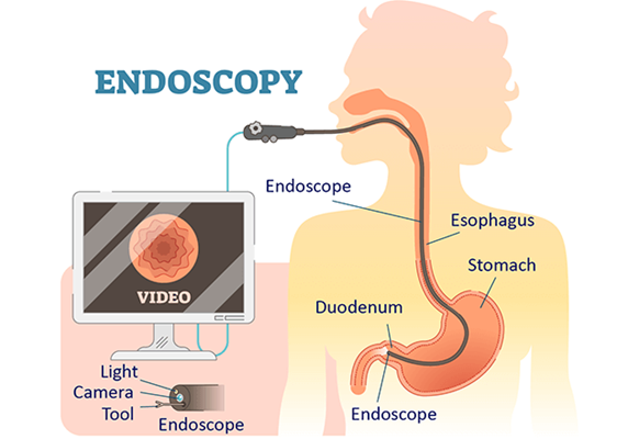
Simultaneous Localization and Mapping (SLAM) systems have become a standard in various technological fields, from autonomous robotics to augmented reality. However, in recent years, this technology has found a particularly unique application in medical imaging– in endoscopic videos. But what is SLAM?
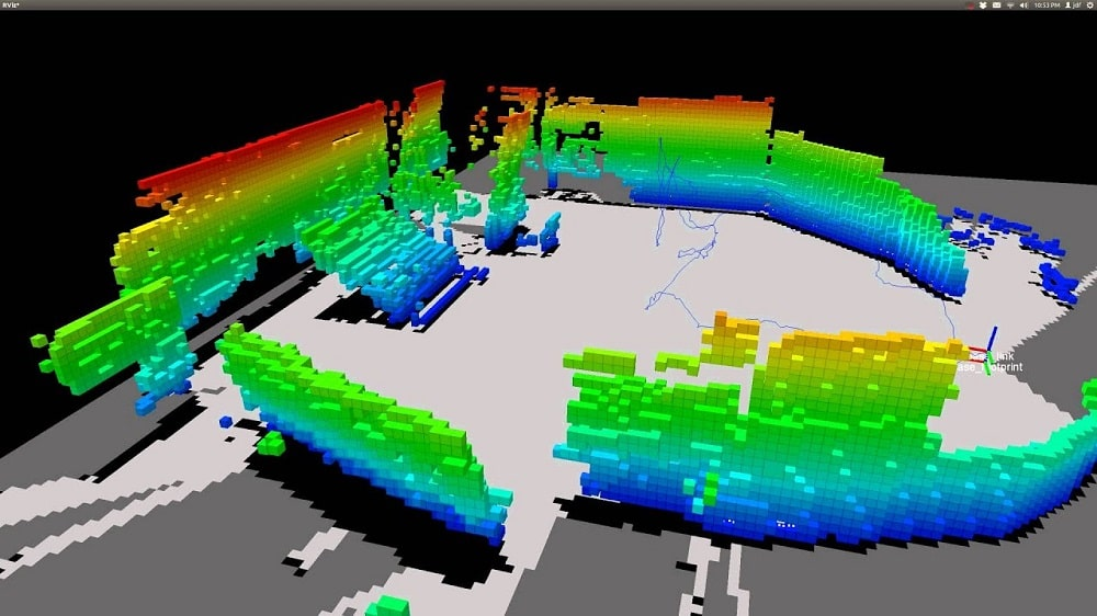
Figure 1: A sample image using SLAM reconstruction from SG News Desk.
SLAM systems were conceptualized in robotics and computer vision for navigation purposes. Before SLAM, the fields employed more elementary methods,
Mapping: the process of creating a representation of an environment, typically in the form of a 2D or 3D map. This was done using grid-based and feature-based methods.
You may be thinking, Krishna, you just described SLAM systems, it sounds like. You are right, but the localizing and mapping were separate processes. So a robot would go through the pains of the Heisenberg principle, i.e., the robot would either localize or map– the or is exclusionary.
It was fairly obvious, but still daunting what the next step in research would be. Before we SLAM dunk our basketball, we must do a few lay-ups and free-throw shoots first.
Precursors to SLAM
Here are some inspirations that contributed to the development of SLAM
Probabilistic robotics: The introduction of probabilistic approaches, such as Bayesian filtering, allowed robots to estimate their position and map the environment with a degree of uncertainty, paving the way for more integrated systems.
Kalman filtering: a mathematical technique for estimating the state of a dynamic system. It allowed for continuous estimation of a robot’s position and could be invariant to noisy sensor data.
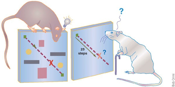
Cognitive Mapping in Animals: Research in cognitive science and animal navigation provided theoretical inspiration, particularly the idea that animals build mental maps of their environment while simultaneously keeping track of their location.
Figure 3: Spatial behavior and cognitive mapping of mice with aging. Image from Nature.
SLAM Dunk – A Culmination (some real Vince Carter stuff)
Finally, many researchers agreed that the separation of localizing and mapping was ineffective, and great efforts went into their integration. SLAM was developed. The goal was to enable systems to explore and understand an unknown environment autonomously, they needed to localize and map the environment simultaneously, with each task informing and improving the other.
With its unique ability to localize and map, researchers found SLAM’s use in any sensory device. Some of SLAM’s earlier use were sensor-based; so data would be inputted from range finders, sonar, and LIDAR; in the late 80s and early 90s. It is good to note that the algorithms were computationally intensive– and still are.
As technology evolved, a vision-based SLAM emerged. This shift was inspired by the human visual system, which navigates the world primarily through sight, enabling more natural and flexible mapping techniques.
Key Milestones
With the latest iterations of SLAM being exponentially better than the origin, it is important to recognize the journey. Here are notable SLAM systems:
EKF-SLAM (Extended Kalman Filter SLAM): One of the earliest and most influential SLAM algorithms, EKF-SLAM, laid the foundation for probabilistic approaches to SLAM, allowing for more accurate mapping and localization.
FastSLAM: Introduced in the early 2000s, FastSLAM utilized particle filters, making it more efficient and scalable. This development was crucial in enabling real-time SLAM applications.
Visual SLAM: The transition to vision-based SLAM in the mid-2000s opened new possibilities for the technology. Visual SLAM systems, such as PTAM (Parallel Tracking and Mapping), enabled more detailed and accurate mapping using standard cameras, a significant step toward broader applications.
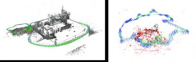
Figure 4: Left LSD-SLAM, right ORB-SLAM. Image found in fzheng.me
From Robotics to Endoscopy (Medical Vision)
As SLAM technology matured, researchers explored its potential beyond traditional robotics. Medical imaging, particularly endoscopy, presented a fantastic opportunity for SLAM. Endoscopy is a medical procedure involving a flexible tube with a camera to visualize the body’s interior, often within complex and dynamic environments like the gastrointestinal tract.
It is fairly trivial why SLAM could be applied to endoscopic and endoscopy-like procedures to gain insights and make more medically informed decisions. Early work focused on using visual SLAM to navigate the gastrointestinal tract, where the narrow and deformable environment presented significant challenges.
One of the first successful implementations involved using SLAM to reconstruct 3D maps of the colon during colonoscopy procedures. This approach improved navigation accuracy and provided valuable information for diagnosing conditions like polyps or tumors.
Researchers also explored the integration of SLAM with other technologies, such as optical coherence tomography (OCT) and ultrasound, to enhance the quality of the maps and provide additional layers of information. These efforts laid the groundwork for more advanced SLAM systems capable of handling the complexities of real-time endoscopic navigation.
Figure 6: Visual of Optical Coherence Tomography from News-Medical.
Endoscopy SLAMs – What Our Group Looked At
As a part of our study, we looked at some presently used and state-of-the-art SLAM systems. Below are the three that various members of our team attempted:
NICER-SLAM (RGB): a dense RGB SLAM system that simultaneously optimizes for camera poses and a hierarchical neural implicit map representation, which also allows for high-quality novel view synthesis.
ORB3-SLAM (RBG): (there is also ORB1 and ORB2) ORB-SLAM3 is the first real-time SLAM library able to perform Visual, Visual-Inertial, and Multi-Map SLAM with monocular, stereo, and RGB-D cameras, using pin-hole and fisheye lens models. In all sensor configurations, ORB-SLAM3 is as robust as the best systems available in the literature and significantly more accurate.
DROID-SLAM (RBG): a new deep learning-based SLAM system. DROID-SLAM consists of recurrent iterative updates of camera pose and pixel-wise depth through a Dense Bundle Adjustment layer.
Some other SLAM systems that our team would have loved to try our hand at are:
Gaussian Splatting SLAM: first application of 3D Gaussian Splatting in monocular SLAM, the most fundamental but the hardest setup for Visual SLAM.
GlORIE-SLAM: Globally Optimized RGB-only Implicit Encoding Point Cloud SLAM. This system uses a deformable point cloud as the scene representation and achieves lower trajectory error and higher rendering accuracy compared to competitive approaches.
This concludes part 1 of What it Takes to Get a SLAM Dunk. This post should have given you a gentle, but robust-enough introduction to SLAM systems. Vince Carter might even approve.
Figure 9: An homage to Vince Carter, arguably the greatest dunk-er ever. Image from Bleacher Report.
Primary mentors: Silvia Sellán, University of Toronto and Oded Stein, University of Southern California
Volunteer assistant: Andrew Rodriguez
Fellows: Johan Azambou, Megan Grosse, Eleanor Wiesler, Anthony Hong, Artur RB Boyago, Sara Samy
After talking about what are some of the ways to reconstruct sdfs (see part one), we now study the question of how to evaluate their performance. Two classes of error function are considered, the first more inherent to our sdf context, and the second more general in all situations. We will first show results by our old friends, Chamfer distance, Hausdorff distance, and area method (see here for example), and then introduce the inherent one.
Hausdorff and Chamfer Distance
The Chamfer distance provides an average-case measure of the dissimilarity between two shapes. It calculates the sum of the distances from each point in one set to the nearest point in the other set. This measure is particularly useful when the goal is to capture the overall discrepancy between two shapes while being less sensitive to outliers. The Chamfer distance is defined as: $$ d_{\mathrm{Chamfer }}(X, Y):=\sum_{x \in X} d(x, Y)=\sum_{x \in X} \inf _{y \in Y} d(x, y) $$
The Bi-Chamfer distance is an extension that considers the average of the Chamfer distance computed in both directions (from \(X\) to \(Y\) and from \(Y\) to \(X\) ). This bidirectional measure provides a more balanced assessment of the dissimilarity between the shapes: $$ d_{\mathrm{B} \mathrm{-Chamfer }}(X, Y):=\frac{1}{2}\left(\sum_{x \in X} \inf {y \in Y} d(x, y)+\sum{y \in Y} \inf _{x \in X} d(x, y)\right) $$
The Hausdorff distance, on the other hand, measures the worst-case scenario between two shapes. It is defined as the maximum distance from a point in one set to the closest point in the other set. This distance is particularly stringent because it reflects the largest deviation between the shapes, making it highly sensitive to outliers.
The formula for Hausdorff distance is: $$ d_{\mathrm{H}}^Z(X, Y):=\max \left(\sup {x \in X} d_Z(x, Y), \sup {y \in Y} d_Z(y, X)\right) $$
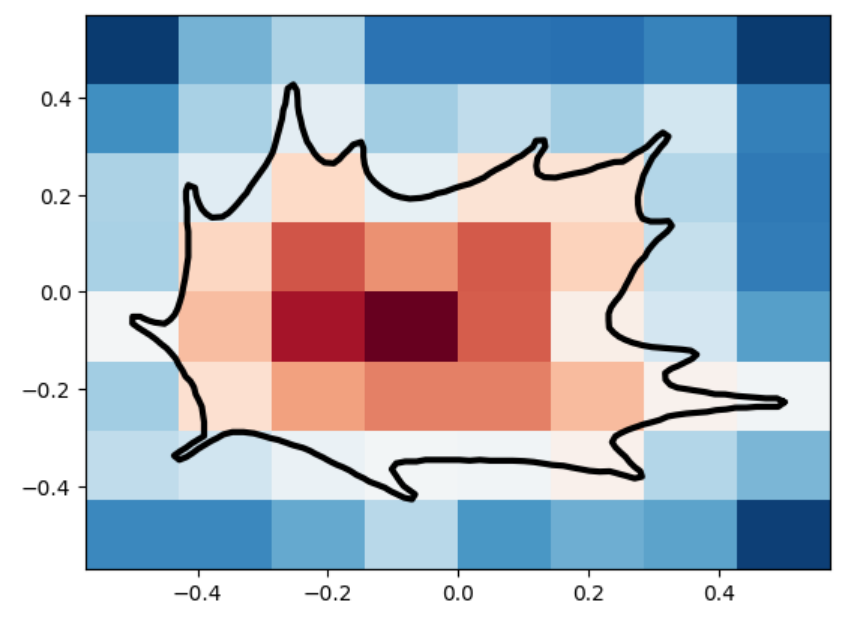
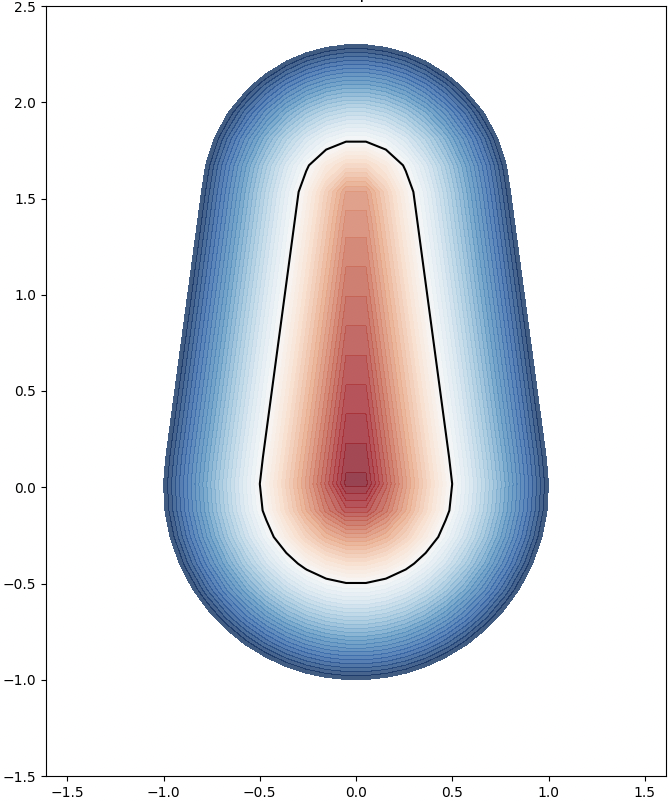
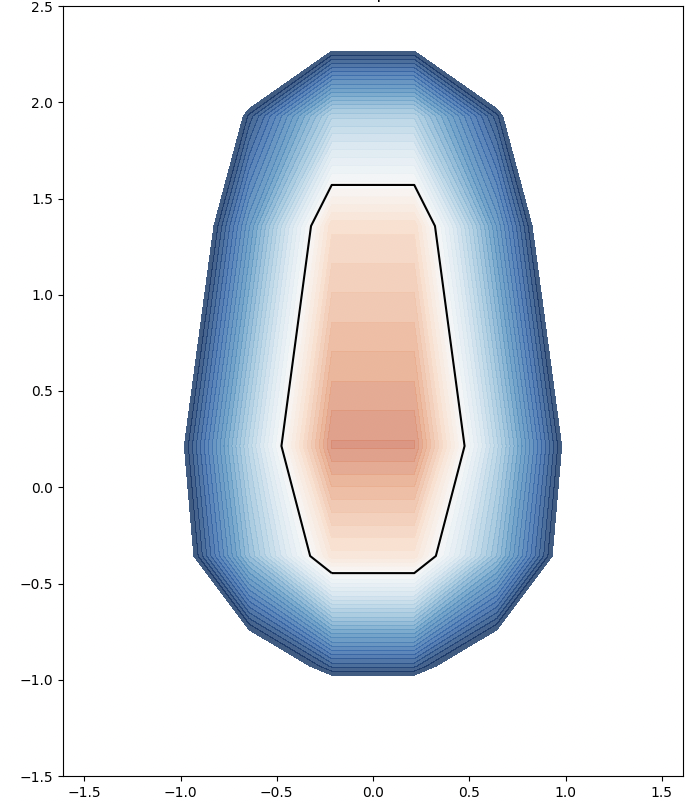
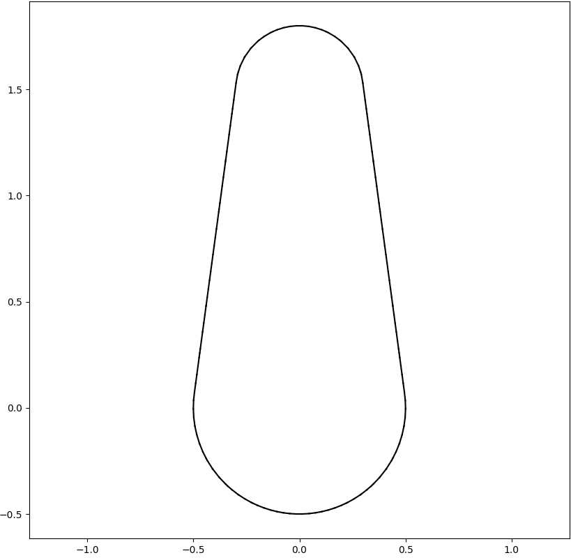
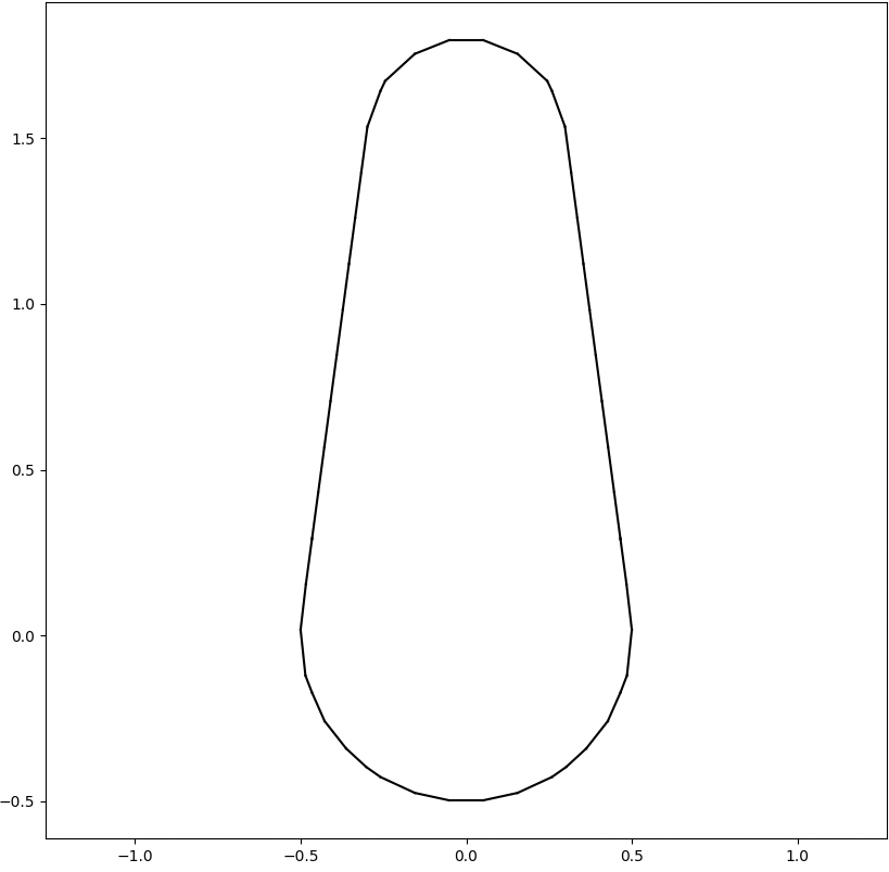
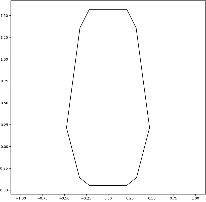
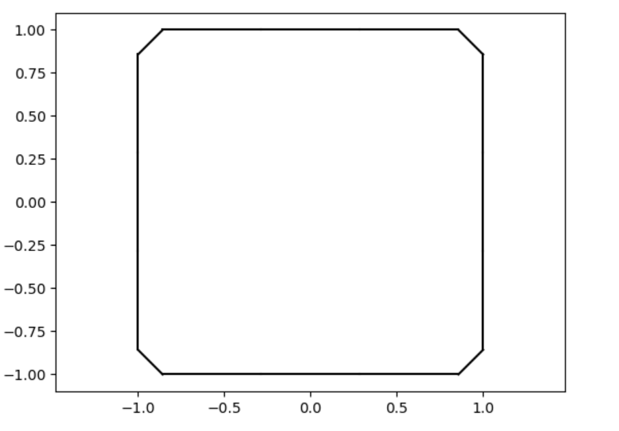
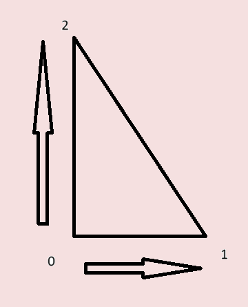
We analyze the Hausdorff distance for the uneven capsule (the shape on the right; exact sdf taken from there) in particular.
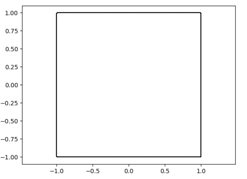
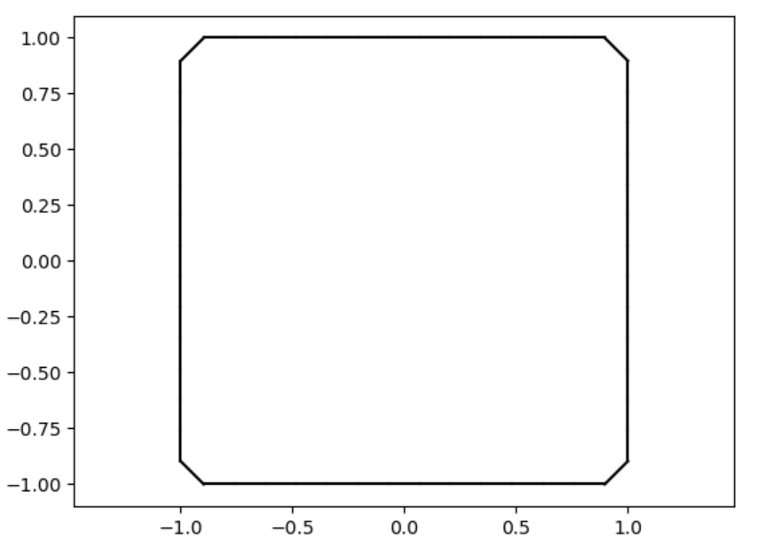
This plot visually compares the original zero level set (ground truth) with the reconstructed polyline generated by the marching squares algorithm at a specific resolution. The black dots represent the vertices of the polyline, showing how closely the reconstruction matches the ground truth, demonstrating the efficacy of the algorithm at capturing the shape’s essential features.
This plot shows the relationship between the Hausdorff distance and the resolution of the reconstruction. As resolution increases, the Hausdorff distance decreases, illustrating that higher resolutions produce more accurate reconstructions. The log-log plot with a linear fit suggests a strong inverse relationship, with the slope indicating a nearly quadratic decrease in Hausdorff distance as resolution improves.
Area Method for Error
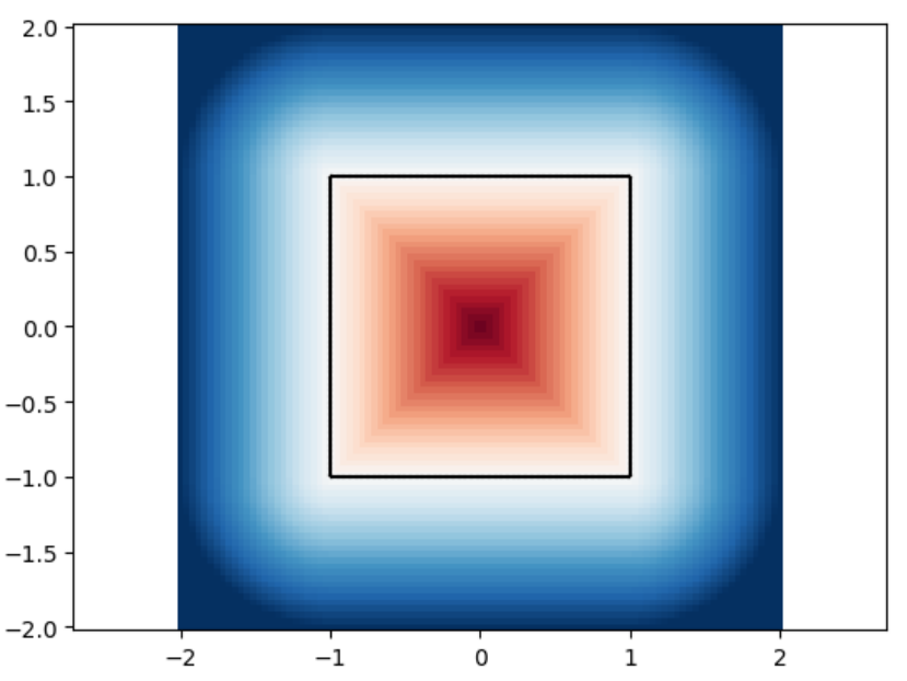
Another error method we explored in this project is an area-based method. To start this process, we can overlay the original polyline and the generated polyline. Then, we can determine the area between the two, counting all regions as positive area. Essentially, this means that if we take values inside a polyline to be negative and outside a polyline to be positive, the area counted as error consists of the set of all regions where the sign of the original polyline’s SDF is not equal to the sign of the generated polyline’s SDF. The resultant area corresponds to the error of the reconstruction.
Here is a simple example of this area method using two quadrilaterals. The area between them is represented by their union (all blue area) with their intersection (the darker blue triangle) removed:
Here is an example of the area method applied to a star, with the area quantity corresponding to error printed at the top:
Inherent Error Function
We define the error function between the reconstructed polyline and the zero level set (ZLS) of a given signed distance function (SDF) as: $$ \mathrm{Error}=\frac{1}{|S|} \sum_{s \in S} \mathrm{sdf}(s) $$
Here, \(S\) represents a set of sample points from the reconstructed polyline generated by the marching squares algorithm, and \(|\mathrm{S}|\) denotes the cardinality of this set. The sample points include not only the vertices but also the edges of the reconstructed polyline.
The key advantage of this error function lies in its simplicity and directness. Since the SDF inherently encodes the distance between any query point and the original polyline, there’s no need to compute distances separately as required in Hausdorff or Chamfer distance calculations. This makes the error function both efficient and well-suited to our specific context, providing a more streamlined and integrated approach to measuring the accuracy of the reconstruction.
Note that one variant one can consider is to square the \(\mathrm{sdf}(s)\) part to get rid of the signed nature, because the signs can cancel with each other for the reconstructed polyline is not always entirely inside the ground truth or entirely cotains the ground truth.
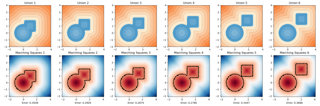
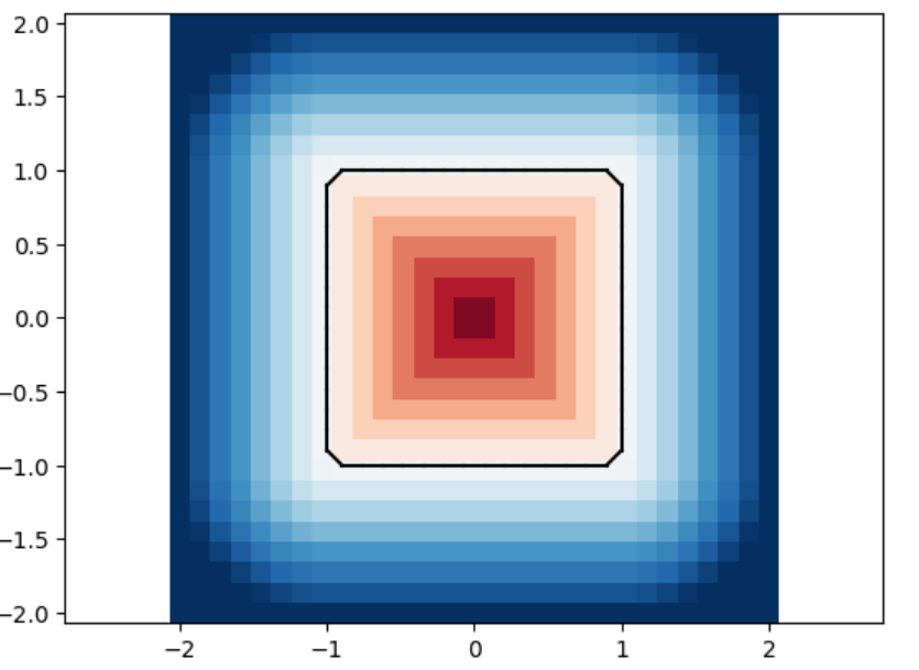
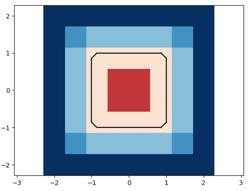
Below are one experiment we did for computing using this inherent error function, the unsquared one. We let the circle sdf be fixed and let the square sdf “escape” from the circle in a constant speed of \(0.2\). That is, we used the union of a fixed circle and a square with changing position as a series of shapes to do analysis. We then draw with color map used in this repo for the ground truths and the marching square results using the common color map.
The inherent error of each union After several trials, one simple observation drawn from this escapaing motion is that when two shapes are more confounding with each other, as in the initial stage, the error is higher; and when the image starts to have two separated connected components, the error rises again. The first one can perhaps be explained by what the paper pointed out as pseudo-sdfs, and the second one is perhaps due to occurence of multipal components.
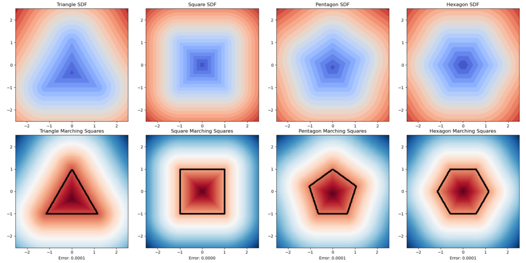
Here is another experiment. We want to know how well this method can simulate the physical characteristics of an object’s rugged level. We used a series of regular polygons. Although the result is theoretically unintheresting as the errors are all nearly zero, this is visually conformting.
Butlerian concerns aside, neural networks have proven to be extremely useful in doing everything we couldn’t think was to be done in this century; extremely advanced language processing, physically motivated predictions, and making strange, artful images using the power of bankrupt corporate morality.
Now, I’ve read and seen a lot of this “stuff” in the past, but I never really studied it, in-depth. Luckily, I got put with four exceedingly capable people in the area, and now manage to write a tabloid on the subject. I’ll write down the very basics of what I learned this week.
Taylor’s theorem
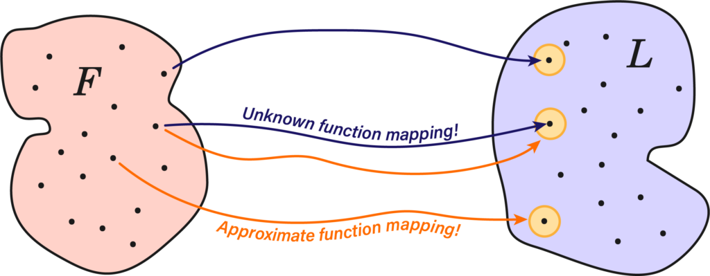
Suppose we had a function \( f : F \rightarrow L \) between the feature space \(F\) and a label space \(L\), both of these spaces are composed of a finite set of data points \( x_i \) and \( y_i \), we’ll put them into a dataset \(\mathfrak{D} = \{(x_i, y_i,) \}^N_{i=1} \). This function can represent just about anything as long as we’re capable of identifying the appropriate labels; images, videos and weather patterns.
The issue is, we don’t know anything about \(f\), but we do have a lot of data, so can we construct a arbitrarily good approximation \( f_\theta \) that functions a majority of the time? The whole field of machine learning asks not only if this is possibly, but if it is, how does one produce such a function, and with how much data?
Indeed, such a mapping may be extremely crooked, or of a high-dimensional character, but as long as we’re able to build universal function approximators of arbitrary precision, we should, in principle, be able to construct any such function.
Third-order Taylor approximation for the cubic polynomial \( x^3/7 + cos(x) \) around the point \( x = 3 \).
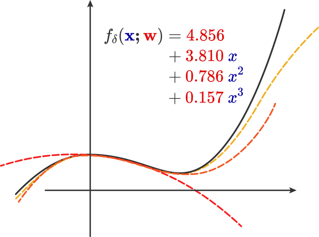
Naively, the first type of function approximator is a machine that produces a Taylor expansion; we call this machine \( f_\delta(\mathbf{x;w}) \) that approximates the real \( f(\mathbf{x})\). It contains the function input \( \mathbf{x}\), and a weight vector \(\mathbf{w}\) containing all of the coefficients of the Taylor expansion. We’ll call this parameter list the weights of the expansion.
Indeed, this same process can be taken up by any asymptotic series that converges onto the result. Now, what we’ve done is that we already had the function and wanted to find this approximation. Can we do the reverse procedure of acquiring a generic third degree polynomial: \[ f_\delta(x) = c_0 + c_1x + c_2 x^2 + c_3 x^3 \]
And then find the weights such that around the chosen point \( \mathbf{x} \) it fits with minimal loss? This question if of course, a extensively studied area of mathematically approximating/interpolating/extrapolating functions, and also the motivating factor for a NN, they’re effectively more complicated versions of this idea using a different method of fitting these weights, but it’s the same principle of applying a arbitrarily large number of computations to get to some range of values.
The first issue is that the label and feature spaces are enormously complicated, their dimensionality alone poses a formidable challenge in making a process to adjust said weights. Further, the structure in many of these spaces is not captured by the usual procedures of approximation. Taylor’s theorem, as our hanged man, is not capable of approximating very crooked functions, so that alone discards it, but
Thought(Thought(Thought(…)))
A neural network is the graphic representation of our neural function \(f_\theta\). We will define two main elements: a simple affine transform \(L = \mathbf{A}_i \mathbf{x} + \mathbf{b}_i \), and a activation function \( \sigma(L\), which can be any function, really, including a polynomial, but we often use a particular set of functions that are useful for NNs, such as a ReLu or a sigmoidal activation.
We can then produce a directed graph that shows the flow of computations we perform on our input \( \mathbf{x}\) across the many neurons of this graph. In this basic case, we have that the input \(x\) is feed onto two distinct neurons. The first transformation is \( \sigma_1(A_1x+b_1) \), whose result, \(x_1\), is feed onto the next neuron; the total result is a composition of the two transforms \(f \circ g = \sigma_2(A_2(f)+b_2 = \sigma_2(A_2(\sigma_1(A_1x+b_1))+b_2) \).
The total result of this basic net on the right is then \(\sigma_3(z) + \sigma_5(w) \), where \(w\) is the result of the transformations in the left, and \(z\) the ones on the right. We could do a labeling procedure and see then that the end result is of the form of a direct composition across the right layer of the affine transforms \((A, B, C)\) and activation functions \( (\sigma_1, \sigma_2, \sigma_3 \), and of the left hand side affine transforms \( (D, E, F) \) and functions \( (\sigma_4, \sigma_5, \sigma_6 ) \), which provides a 12-dimensional weight vector \( \mathbf{w} \):
\[ f_\theta(\mathbf{x;w}) = (\sigma_3\circ C \circ \sigma_2 \circ B \circ \sigma_1 \circ A) + (\sigma_6 \circ F \circ \sigma_5 \circ E \circ \sigma_4 \circ D) \]
Once again, the idea is that we can retrofit the coefficients of the affine transforms and activation functions to express different function approximations; different weight vectors yield different approximations. Finding the weights is called the training of the network and is done by an automatic process.
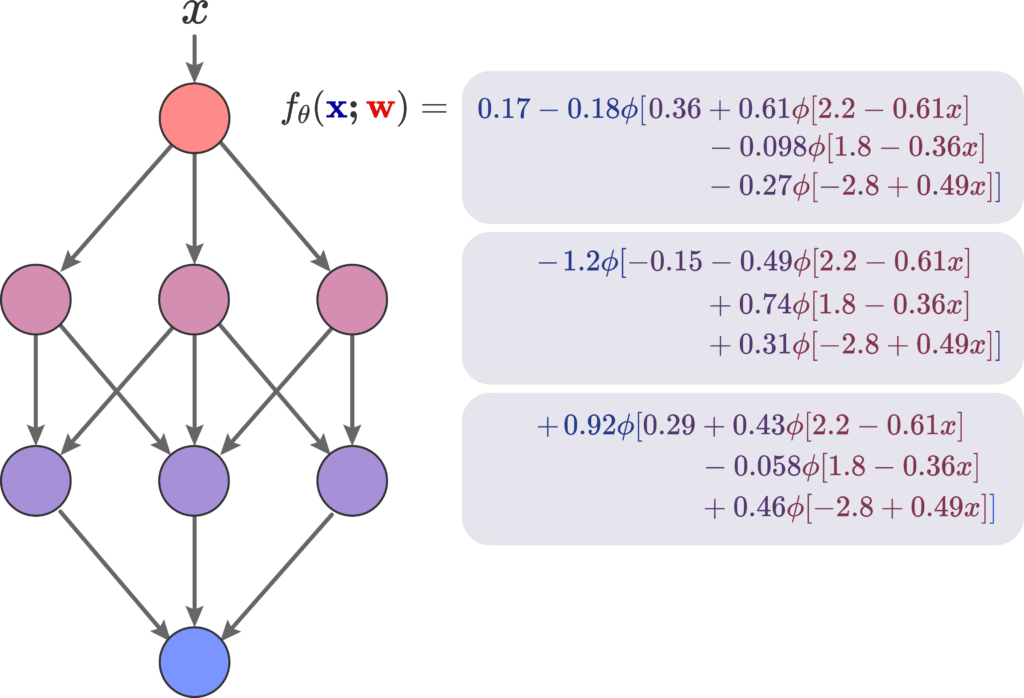
A feed forward NN is a deep, meaning it has more than intermediate layer, neural function \( f_\theta(\mathbf{x;w}) \) that, given some affine transformation \(f\) and activation function \(f\), is defined by:
Here we see a basic FF neural function \( f_\theta (\mathbf{x, w}) \) and its corresponding neural network representation; it has a depth of 4 and a width of 3. The input \( x\) is feed into a singular neuron, that doesn’t change it, and its then feed to three distinct neurons, each with its own weights for the affine transformation, and this all repeats until the last neuron. All of them have the same underlying activation function \( \phi\):
If we actually go out and compute this particular neural function using \( \phi \) as the sigmoid function, we get the approximation of a sine wave. Therefore, we have sucessfully approximated a low dimensional function using a NN How did we, however, get these specifics weights? By means of gradient descent. Maybe I’ll write something about the trainings of NNs as I learn more about them.
Equivariant NNs
Now that we approximated a simple sine wave, the obvious next step is the three dimensional reconstruction of a mesh into a signed distance function.
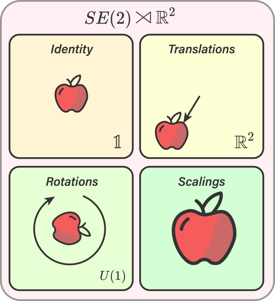
But since I don’t actually know the latter, I’ll go to the non-obvious next step of looking at the image of an apple. If we were to perform a transformation on said apple as either a translation, rotation, or scaling, ideally our neural network should be able to still identify the data as an apple. This means we somehow need to encode the symmetry information onto the weights of the network. This breeds the principle of an equivariant NN, studied in the field of geometrical deep learning.
I’ll try to study these later to make more sense about them as well.
Author: Ehsan Shams (Alexandria Univerity, Egypt) Project Mentor: Sofia Di Toro Wyetzner (Stanford University, USA) Volunteer Teaching Assistant: Shanthika Naik (CVIT, IIIT Hyderabad, India)
In my first SGI research week, I went on a fascinating exploratory journey into the world of splines under the guidance of Sofia Wyetzner, and gained an insight into how challenging yet intriguing their construction can be especially under tight constriants such as the requirement for a closed-form expression for their arc-length. This specific construction was the central focus of our inquiry, and the main drive for our exploration.
Splines are important mathematical tools for they are used in various branches of mathematics, including approximation theory, numerical analysis, and statistics, and they find applications in several areas such as Geometry Processing (GP). Loosely speaking, such objects can be understood as mappings that take a set of discrete data points and produce a smooth curve that either interpolates or approximates these points. Thus, it becomes natural immediately to see that they are of great importance in GP since, in the most general sense, GP is a field that is mainly concerned with transforming geometric data1 from one form to another. For example, splines like Bézier and B-spline curves are foundational tools for curve representation in computer graphics and geometric design (Yu, 2024).
Having access to arc lengths for splines in GP is essential for many tasks, including path planning, robot modeling, and animation, where accurate and realistic modeling of curve lengths is critically important. For application-driven purposes, having a closed formula for arc-length computation is highly desirable. However, constructing splines with this arc-length property that can interpolate \( k \) arbitrary data points reasonably well is indeed a challenging task.
Our mentor Sofia, and Shanthika guided us through an exploration of a central question in spline formulation research, as well as several related tangential questions:
Our central question was:
Given \( k \) points, can we construct a spline that interpolates these points and outputs the intermediate arc-lengths of the generated, curve, with some continuity at control points?
And the tangential ones were:
1. Can we achieve \( G^1 \) / \( C^1\) / \( G^2 \) / \(C^2\) continuity at these points with our spline? 2. Given \(k\) points and a total arc-length, can we interpolate these points with the given arc-length in \( \mathbb{R}^2 \)?
In this article, I will share some of the insights I gained from my first week-long research journey, along with potential future directions I would like to pursue.
Understanding Splines and their Arc-length
What are Splines?
A spline is a mapping \( S: [a,b] \subset \mathbb{R} \to \mathbb{R}^n \) defined as:
where \( a = t_0 < t_1 < \cdots < t_n = b \), and \( s_i: [t_i, t_{i+1}] \to \mathbb{R}^n \) are defined such that, \(S(t)\) ensures \( C^k \) continuity at each internal point \( t_j \), meaning:
\( s_{i-1}^{(m)}(t_j) = s_i^{(m)}(t_j) \) for \( m = 0,1 \dots, k \)
where \( s_{i-1}^{(m)} \) and \( s_i^{(m)} \) are the \( m \)-th derivatives of \( s_{i-1}(t) \) and \( s_i(t) \) respectively.
In other words, a spline is a mathematical construct used to create a smooth curve \( S(t) \) by connecting a sequence of simpler piecewise segments \( s_i(t) \) in a continuous manner. These segments \( s_i(t) \) for \( i = 1, 2, \ldots, n \) are defined on subintervals \( [t_i, t_{i+1}] \) of the parameter domain, and are carefully joined end-to-end. The transitions at the junctions \( \{ t_i \}_{i=1}^{n-1} \) (also known as control points) maintain a desired level of smoothness, typically defined by the continuity of derivatives up to order \( k \) on \( \{s_i(t)\}_{i=1}^n \).
One way to categorize splines is based on the types of functions \(s_i\) they incorporate. For instance, some splines utilize polynomial functions such as Bézier splines and B-splines, while others may employ trigonometric functions such as Fourier splines or hyperbolic functions. However, the most commonly used splines in practice are those based on polynomial functions, which define one or more segments. Polynomial splines are particularly valuable in various applications because of their computational simplicity and flexibility in modeling curves.
Arc Length Calculation
Intuitively, the notion of arc-length of a curve2 can be understood as the numerical measurement of the total distance traveled along the curve from one endpoint to another. This concept is fundamental in both calculus and geometry because it provides a way to quantify the length of some curves, which may not be a straight line. To calculate the arc length of smooth curves, we use integral calculus. Specifically, we apply a definite integral formula – (presented in the following theorem) but, let us first define the concept formally.
Definition. Let \( \gamma : [a, b] \to \mathbb{R}^n \) be a parametrized curve, and \( P = \{ a = t_0, t_1, \dots, t_n = b \} \) a partition of \( [a, b] \). The polygonal approximate3 length of \( \gamma \) from \(P\) is given by the sum of the Euclidean distances between the points \( \gamma(t_i)\) for \( i = 0, 1, \dots, n \):
where \( | \cdot | \) denotes the Euclidean norm in \( \mathbb{R}^n \). This polygonal approximation becomes a better estimate of the actual length of the curve as the partition \( P\) becomes finer (i.e., as the maximum distance between successive \( t_i \) tends to zero). The actual length of the curve can be defined as:
\( L(\gamma) = \sup_P L_P(\gamma) \)
If the curve \( \gamma \) is sufficiently smooth, the actual length of the curve can be computed using definite integration as shown in the following theorem.
Arc Length Theorem. Let \( \gamma : [a, b] \to \mathbb{R}^n \) be a \( C^1 \) curve. The arc length \( L(\gamma) \) of \(\gamma\) is given by:
\( L(\gamma) = \int_a^b |\gamma'(t)| \, dt \)
where \(\gamma'(t) \) is the derivative of \(\gamma\) with respect to \(t\).
The challenge
As mentioned earlier, in the context of spline construction for GP tasks, ideally one is interested in constructing splines that have closed-form solutions for their arc length (a formula for computing their arc-length). However, curves with this property for their arc-length are relatively rare because the arc length integral often leads to elliptic integrals4 or other forms that do not have elementary antiderivatives. However, there are some curves for which the arc length can be computed exactly using a closed formula. Here are some examples: Straight lines, circles, and parabolas under certain conditions have closed-form solutions for arc length.
Steps to tackle the central question …
Circular Splines: A Starting Point.
In day one, our mentor Sofia went with us through a paper titled “A Class of \(C^2 \) Interpolating Splines” (Yuksel, 2020). In this work, the author introduces a novel class of non-polynomial parametric splines to interpolate given \( k \) control points. Two components define their class construction: interpolating functions and blending functions (defined later). Each interpolating function \(F_j \in \{F_i \}_{i=1}^n\) defines three consecutive control points, and the blending functions \( \{ B_i \}_{i=1}^m \) combines each two consecutive interpolating functions, forming a smooth curve between two control points. The blending functions are chosen so that \( C^2 \)-continuity everywhere is ensured independent of the choice of the interpolating functions. They use trignometric blending functions.
This type of formulation was constructed to attain some highly desirable properties in the resulting interpolating spline not previously demonstrated by other spline classes, including \( C^2 \) continuity everywhere, local support, and the ability to guarantee self-intersection-free curve segments regardless of the placement of control points and form perfect circular arcs. This paper served as a good starting point in light of the central question under consideration because among the interpolating functions they introduce in their paper are circular curves which have closed formulas for arc-length computation. In addition, it gives insight into the spline formulation practice. However, circular interpolating functions are not without their limitations; their constant curvature makes them difficult to reasonably interpolate arbitrary data, and they look bizarre sometimes.
Interesting note: The earliest documented reference – to the best of my knowledge – discussing the connection of two interpolating curves with a smooth curve dates back to Macqueen’s research in 1936 (MacQueen, 1936) Macqueen’s paper, titled “On the Principal Join of Two Curves on a Surface,” explores the concept of linking two curves on a surface.
Here is a demo constructed by the author to visualize the resulting output spline from their class with different interpolating functions, and below is me playing with the different interpolating functions, and looking at how bizarre the circular interpolating function looks when you throw out data points in an amorphus way.
While playing with the demo, the Gnomus musical track by Modest Mussorgsky was playing in parallel in the back of my mind so I put there for you too. It is a hilarious coincidence that the orchestra goes mad when it is the circular spline’s turn to interpolate the control points, and it does so oddly and bizarrely than the other splines in question. It even goes beyond the boundary of the demo. Did you notice that? 🙂
By the end of the day, I was left with two key inquiries, and a starting point for investigating them:
How do we blend desirable interpolating functions to construct splines with the properties we want? Can we use a combination of circular and elliptical curves to achieve more flexible and accurate interpolation for a wider variety of data points while maintaining a closed form for their arc length? What other combinations could serve us well? I thought to myself: I should re-visit my functional analysis course as a starting point to think about this in a clear way.
From day two to five, we followed a structured yet not restrictive approach, akin to “we are all going to a definite destination but at the same time, everyone could stop by to explore something that captured their attention along the way if they want to and share what intrigued them with others”. This approach was quite effective and engaging:
Implementing a User-Interactive: Our first task was to develop a simple user interface for visualizing existing spline formulations. My SGI project team and friends—Charuka Bandara, Brittney Fahnestock, Sachin Kishan,and I—worked on this in Python (for Catmull-Rom splines) and MATLAB (for Cubic and Quadratic splines). This tool allowed us to visualize how different splines behave and change shape whenever the control points change, also restored my love for coding as I have not coded in a while … you know nothing is more joyful than watching your code executing exactly what you want it to do, right? Below is a UI for visualizing a Cubic Spline. Find the UI for the Quadratic Spline, and the Catmull-Rom here.
Interactive Cubic Spline
Exploring Blending Functions Method: As a natural progression towards our central inquiry, and a complementary task to reading Yuksel’s paper, we eventually found our way to exploring blending functions—a topic I had been eagerly anticipating.
Here, I decided to pause and explore more about the blending function method in spline formulation.
The blending function method, is a method that provides a way to construct a spline \( S(t) \) as a linear combination of a set of control points \( \{p_i(t)\}_{i=1}^n \) and basis functions (blending functions) \( \{B_i(t)\}_{i=1}^n \) in the following manner:
\( S(t) = \sum_{i=1}^n p_i B_i(t)\) (*)
where: \( t \): is the parameter defined over the interval of interest \( [a,b] \)
These blending functions \(B_i(t)\) typically exhibit certain properties that govern, for example, the smoothness, continuity, shape, and preservation of key characteristics that we desire in the resulting interpolating splines. Thus, by carefully selecting and designing those blending functions, it is possible to tailor the behaviour of spline interpolation to meet the specific requirements and achieve desired outcomes.
Below are some of the properties of important blending functions:
Partition of Unity: \( \sum_{i=1}^n B_i(t) =1, \forall t \in [a,b] \), also called coordinate system independent. This property is important because it provides a convex combination of the control points in question, and this is something you need to ensure that the curve does not change if the coordinate changes, one way to visualize this is by imagining that the control points in questions are beads sitting in an amorphous manner on a sheet of paper and the interpolating curve as a thread going through them, and you move the sheet of paper around, what we need is that the thread that goes through these beads does not move around as well, and this is what this property means. Notice that if you pick an arbitrary set of blending functions, this property is not immediately actualized, and the curve would change.
Local Support: Each blending function \( B_i(t) \neq 0 \forall t \in I and i=1,2, … , n \) where \(I \subset [a,b] \) is the interval of interest and vanishes everywhere else on the domain. This property is important because it ensures computational efficiency. With this property actualized in one’s blending functions, one does not have to worry about consequences on their interpolating curve if they are to modify one control point .. for it will only affect a local region in the curve, and not the entire curve.
Non-negativity: Blending functions are often non-negative over the domain of definition \( [a,b] \). This property is called convex hull. It is important for maintaining stability and predictability of the interpolating spline. It prevents the curve from oscillating wildly or provides unfaithful representation of the data point in question.
Smoothness: Blending functions dictate the overall smoothness of the resulting spline since the space of \( C^k (\mathcal{K})\) ( \(k\)-times continously differentiable functions defined on a closed and compact set \(\mathcal{K}\) is a vector space over \(\mathbb{R}\) or \(\mathbb{C}\).
Symmetry: Blending functions that are symmetric about the central control point, do not change if the points are ordered in reverse. In this context, symmetry is assured, if and only if, \( \sum_{i=1}^n B_i(t) p_i = \sum_{i=1}^n B_i ((a+b)-t) p_{n-i} \) this holds if \(B_i(t) = B_{n-i}((a+b)-t) \). For instance, Timmer’s parametric cubic, and Ball’s cubic – (a variant of cubic Bézier) – curve obey this property.
In principle, there can be as many properties imposed on the blending functions depending on the desired aspects one wants in their interpolating spline \( S(t) \).
Remark. The spline formulation (*) describes the weighted sum of the given control points \( \{p_i\}_{i=1}^n\). In other words, each control point is influencing the curve by pulling it in its direction, and the associated blending function is what determines the strength of this influence and pull. Sometimes, one does not need to use blending functions in trivial cases.
Brain-storming for new spline formulation: Finally, we were prepared for our main task. We brainstormed new spline formulations, in doing so, we first looked at different interpolating curves such as catenaries, parabolas, circles for interpolation and arc-length calculation, explored \(C^1\) and \( C^2 \) continuity at control points, did the math on papers, which something I miss nowadays, for the 3-point, and then laid down the foundation for the \(k\)-point interpolation problem. I worked with the parabolas because I love them.
In parallel, I looked a bit into tangential question two … it is an interesting question:
Given \(k\) points and a total arc-length \(L\), can we interpolate these points with the given arc-length in \(\mathbb{R}^2 \)?
From the polynomial interpolation theorem, we know that for any set of \( k \) distinct points \((x_1, y_1), (x_2, y_2), \ldots, (x_k, y_k) \in \mathbb{R}^2 \), there exists a polynomial \( P(x) \) of degree \( k-1 \) such that: \(P(x_i) = y_i \text{ for } i = 1, 2, \ldots, k.\). Such a polynomial is smooth and differentiable (i.e., it is a \( C^\infty \) function) over \( \mathbb{R} \) thus rectifiable so it possesses a well-defined finite arc-length over any closed interval.
Now, let us parameterize the polynomial \( P(x) \) as a parametric curve \( \mathbf{r}(t) = (t, P(t)) \), where \( t \) ranges over some interval \([a, b] \subset \mathbb{R}\).
Now let us compute its arc-length,
The arc-length \( S \) of the curve \( \mathbf{r}(t) = (t, P(t)) \) from \( t = a \) to \( t = b \) is given by:
\( S = \int_a^b \sqrt{1 + \left(\frac{dP(t)}{dt}\right)^2} \, dt. \)
To achieve the desired total arc-length \( L \), we rescale the parameter \( t \). Define a new parameter \( \tau \) as: \( \tau = \alpha t. \)
Now, the new arc-length ( S’ ) in terms of \( \tau \) is:
\(S’ = \frac{S}{\alpha}.\). To ensure \( S’ = L \), choose \( \alpha = \frac{S}{L} \).
Thereby, by appropriately scaling the parameter \( t \), we can adjust the arc-length to match \( L \). Thus, there exists a curve \( C \) that interpolates the \( k \geq 2 \) given points and has the total arc-length \( L \) in \( \mathbb{R}^2 \).
Now, what about implementation? how could we implement an algorithm to execute this task?
It is recommended to visualize your way through an algorithm on a paper first, then formalize to words and symbols, make sure there are no semantic errors in the formalization then code then debug. You know debugging is one of the most intellectually stimulating exercises, and exhausting ones. I am a MATLAB person so here is a MATLAB function you could use to achieve this task ..
function [curveX, curveY] = curveFunction(points, totalArcLength)
    % Input:
    % points - Nx2 matrix where each row is a point [x, y]
    % totalArcLength - desired total arc length of the curve

    % Output:
    % curveX, curveY - vectors of x and y coordinates of the curve

    % Number of points
    n = size(points, 1);

    % Calculate distances between consecutive points
    distances = sqrt(sum(diff(points).^2, 2));

    % Calculate cumulative arc length
    cumulativeArcLength = [0; cumsum(distances)];

    % Normalize cumulative arc length to range from 0 to 1
    normalizedArcLength = cumulativeArcLength / cumulativeArcLength(end);

    % Desired number of points on the curve
    numCurvePoints = 100; % Change as needed

    % Interpolated arc length for the curve
    curveArcLength = linspace(0, 1, numCurvePoints);

    % Interpolated x and y coordinates
    curveX = interp1(normalizedArcLength, points(:, 1), curveArcLength, 'spline');
    curveY = interp1(normalizedArcLength, points(:, 2), curveArcLength, 'spline');

    % Scale the curve to the desired total arc length
    scale = totalArcLength / cumulativeArcLength(end);
    curveX = curveX*scale;
    curveY = curveY*scale;

    %plot(curveX, curveY);

 % Plot the curve
    figure;
    plot(curveX, curveY);
    hold on;
    title('Curve Interpolation using Arc-Length and Points');
    xlabel('X');
    ylabel('Y');
    grid on;
    hold off;
end
Key Takeaways, and Possible Research Directions:
Key Takeaway:
Splines are important!
Constructing them is nontrivial especially under multiple conflicting constraints, as it significantly narrows the feasible search space of potential representative functions.
Progress in abstract mathematics makes the lives of computational engineers and professionals in applied numerical fields easier, as it provides them with greater spaces for creativity and discoveries of new computational tools.
Possible Future Research Directions:
“I will approach this question as one approaches a
hippopotamus: stealthily and from the side.”
– R. Mahony
I borrowed this quote from Prof. Justin Solomon’s Ph.D. thesis. I read parts of it this morning and found that the quote perfectly captures my perspective on tackling the main question of this project. In this context, the “side” approach would involve exploring the question through the lens of functional analysis. 🙂
Acknowledgments. I would like to express my sincere gratitude to our project mentor Sofia Di Toro Wyetzner and Teaching Assistant Shanthika Naik for their continuous support, guidance, and insights to me and my project fellows during this interesting research journey, which prepared me well for my second project on “Differentiable Representations for 2D Curve Networks”. Moreover, I would like to thank my team fellows Charuka Bandara, Brittney Fahnestock, and Sachin Kishan for sharing interesting papers which I am planning to read after SGI!
Silva, L. and Gay Neto, A. (2023). Geometry reconstruction based on arc splines with application to wheel-rail contact simulation. Engineering Computations, 40(7/8), 1889-1920. https://doi.org/10.1108/ec-11-2022-0666
Yuksel, C. (2020). A class of c 2 interpolating splines. ACM Transactions on Graphics, 39(5), 1-14. https://doi.org/10.1145/3400301
Geometric data refers to information that describes the shape, position, and properties of objects in space. It includes the following key components: curves, surfaces, meshes, volumes ..etc ↩︎
In this article, when we say curves, we usually refer to parametric curves. However, parametrized curves are not the same as curves in general ↩︎
The term “polygonal approximation” should not be taken too literally; The term suggests that the Euclidean distance between two points \(p\) and \(q\) should be the “straight-line” distance between them. ↩︎
Last week SGI welcomed Jesse Louis-Rosenberg, Co-founder and Chief Science Officer at Nervous System, a generative design studio. Inspired by natural pattern formation, Nervous System creates software and computer simulations that famously mimic organic structures to produce unique mediums of art. Since 2007, Nervous System has looked to Laplacian growth and Voronoi structures to develop algorithms that are “generative”, meaning each art piece is one of one.
Recognizing the lost artistry of jigsaw puzzles post the Industrial revolution, Nervous System “hacked” together the idea of a multiphase model of dendritic solidification to create a puzzle cut generation system. The simulation begins with a “seed” that represents the initial piece location, from which it will expand towards its neighbor, until the interlocking structure is formed. The images for the puzzle are created by another cut system, based on the idea of growing elastic rods, where a cellular p-shape’s edges bend and collide to form mazelike patterns. These systems allow for each puzzle to produce a unique combination of patterns. After the puzzles are 3d printed, they are laser cut. In order to avoid flash backs while cutting, each piece undergoes a process of shellability, where the connected components are turned into a local property in the ordering. From there, the computational artists determine which pieces are useable in the final stages of production and distribution.
In 2011, looking to the infamous topology of a Klein Bottle, Nervous System set out to create the infinite galaxy puzzle – a double sided jigsaw that tiles continuously. Due to its lack of a fixed shape, starting point, or edges, the puzzle can be recreated thousands of times without ever producing the same image. Using similar processes, Nervous system also offer hundreds of products from black hyphae lamps to tetra kinematic necklaces.
Today, Nervous System’s art and algorithms can be found everywhere from the Museum of Modern Art in New York to 3D printed organ research at Rice University. It serves as source of inspiration and reminder for researchers to explore the artistic richness at the intersection of design and computation.
Primary mentors: Silvia Sellán, University of Toronto and Oded Stein, University of Southern California
Volunteer assistant: Andrew Rodriguez
Fellows: Johan Azambou, Megan Grosse, Eleanor Wiesler, Anthony Hong, Artur, Sara
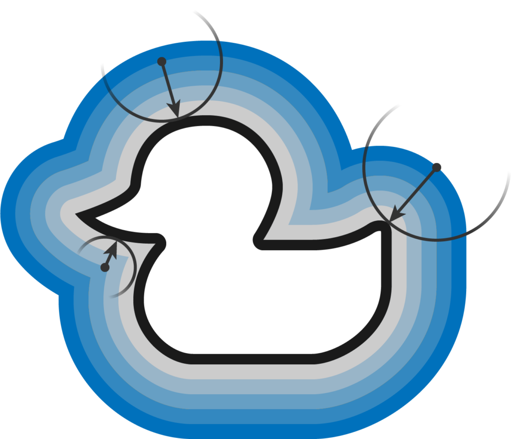
The definition of SDFs using ducks
Suppose that you took a piece of metal wire, twisted into some shape you like, let’s make it a flat duck, and then put it on a little pond. The splash of water made by said wire would propagate as a wave all across the pond, inside and outside the wire. If the speed of the wave were \(1 m/s \), you’d have, at every instant, a wavefront telling you exactly how far away a given point is from the wire.
This is the principle behind a distance field, a scalar valued field \( d(\mathbf{x}) \) whose value at any given point \(\mathbf{x}\) is given by\( d(\mathbf{x}, S) = \min_{\mathbf{y}}d(\mathbf{x}, \mathbf{y})\), where \( S \)is a simpled closed curve. To make this a signed distance field, we can distinguish between the interior and exterior of the shape by adding a minus sign in the interior region.
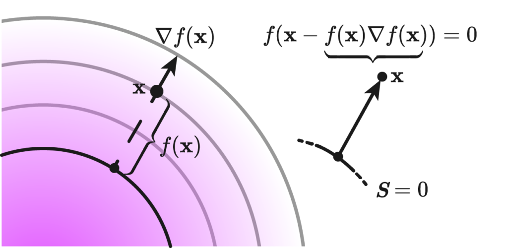
Suppose we were to define sdf without knowing the boundary \(S\); given a region \( \Omega \) and a surface \( S \), whose inside is defined as the closure of \( \overline{\Omega} = A \). A function \( f : \mathbb{R}^n \rightarrow \mathbb{R} \) is said to be a signed distance function if for every point \( \mathbf{x} \in \Omega \) , we have eikonality \( | \nabla f | = 1 \) and closest point condition: \[ f( \mathbf{x} – f(\mathbf{x}) \nabla f(\mathbf{x})) = 0 \]
The statement reads very simply: if we have a point \( \mathbf{x} \), and take the difference vector to the normal of the level set at hand times the distance, it should take us to the point \( \mathbf{x} \) closest to the zero level set.
This second definition is equivalent to the first one by an observation that eikonality implies \(1\)-Lipschitz property of the function \(f\) and it is also used for the last step of the following derivation: \(\exists q \in S:=f^{-1}(0)\) $$ p-f(p) \nabla f(p)=q \Longrightarrow p-q=f(p) \nabla f(p) \Longrightarrow|p-q|=|f(p)| $$
This combined with \(1\)-Lipschitz property gives a proof of contradiction for characterization of sdf by eikonality and closest point condition.
Our project was focused on the SDF-to-Surface reconstruction methods, which is, given a SDF, how can we make a surface out of it? I’ll first tell you about the much simpler problem, which is Surface-to-SDF.
Our SDFs
To lay the foundation, we started with the 2D case: SDFs in the plane from which we can extract polylines. Before performing any tests, we needed a database of SDFs to work with. We created our SDFs using two different skillsets: art and math.
The first of our SDFs were hand-drawn, using an algorithm that determined the closest perpendicular distance to a drawn image at the number of points in a grid specified by the resolution. This grid of distance values was then converted into a visual representation of these distance values – a two-dimensional SDF. Here are some of our hand-drawn SDFs!
The second of our SDFs were drawn using math! Known as exact SDFs, we determined these distances by splitting the plane into regions with inequalities and many AND/OR statements. Each of these regions was then assigned an individual distance function corresponding to the geometry of that space. Here are some of our exact SDF functions and their extracted polylines!
Exact vs. Drawn
Exact Signed Distance Functions (SDFs) provide precise, mathematically rigorous measurements of the shortest distance from any point to the nearest surface of a shape, derived analytically for simple forms and through more complex calculations for intricate geometries. These are ideal for applications demanding high precision but can be computationally intensive. Conversely, drawn or approximate SDFs are numerically estimated and stored in discretized formats such as grids or textures, offering faster computation at the cost of exact accuracy. These are typically used in digital graphics and real-time applications where speed is crucial and minor inaccuracies in distance measurements are acceptable. The choice between them depends on the specific requirements of precision versus performance in the application.
Operations on SDFs
For two SDFs, \(f_1(x)\) and \(f_2(x)\), representing two shapes, we can define the following operations from constructive geometry:
We used these operations to create the following new sdfs: a cat and a tessellation by hexagons.
Marching Squares Reconstructions with Multiple Resolutions
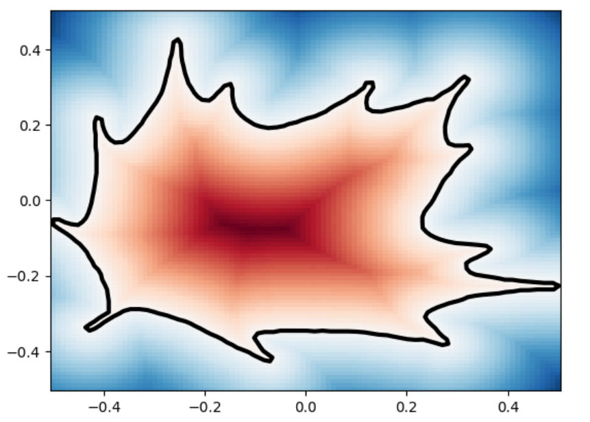
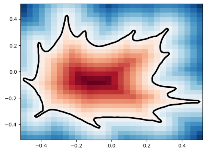
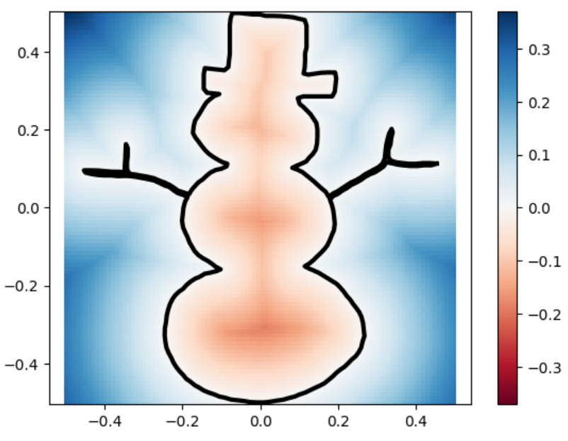
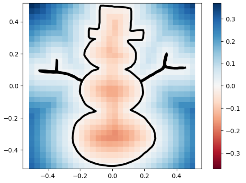
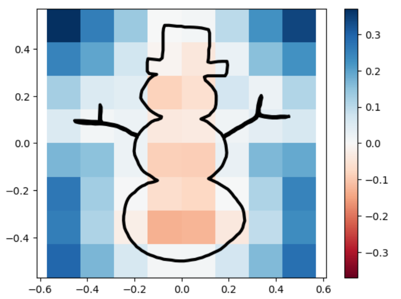
The marching_squares algorithm is a contouring method used to extract contour lines (isocontours) or curves from a two-dimensional scalar field (grid). It’s the 2D analogue of the 3D Marching Cubes algorithm, widely used for surface reconstruction in volumetric data. When applied to Signed Distance Functions (SDFs), marching_squares provides a way to visualize the zero level set (the exact boundary) of the function, which represents the shape defined by the SDF. Below are visualizations of various SDFs which we passed into marching squares with varied resolutions in order to test how well it reconstructs the original shape.
SDF / Resolution
100×100
30×30
8×8
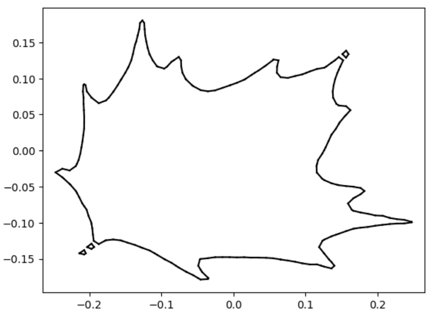
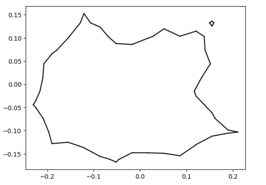
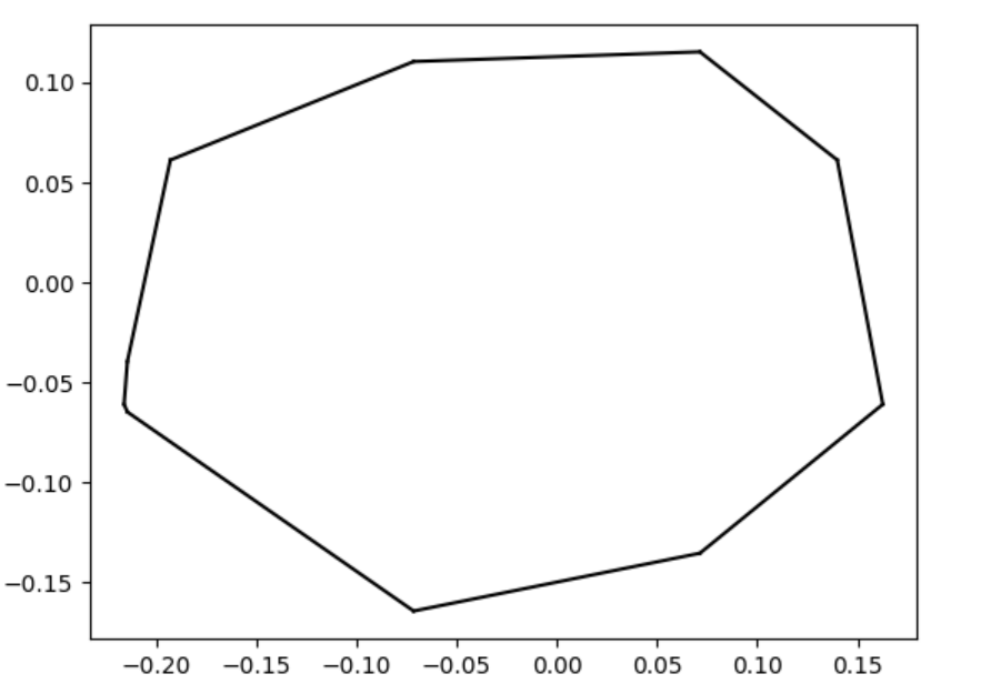
leaf
leaf marching_squares
uneven capsule
uneven capsule marching_squares
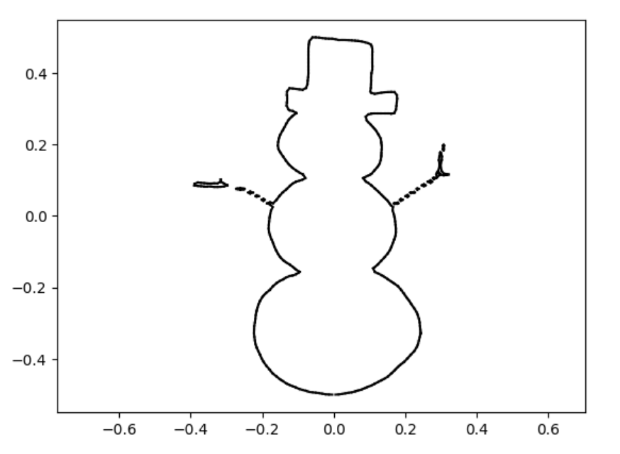
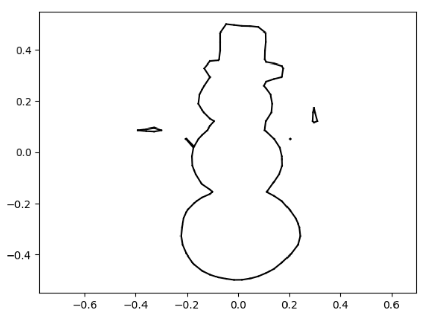
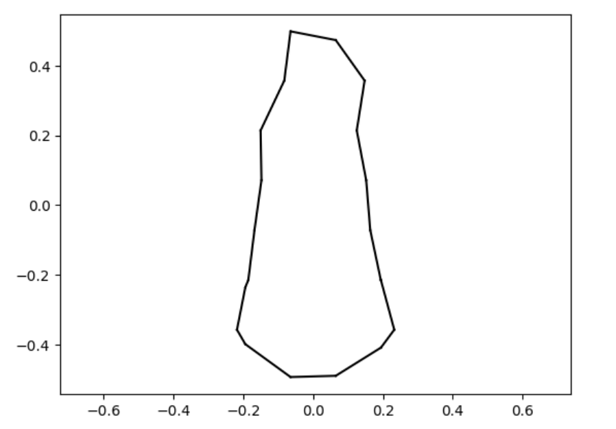
snowman
snowman marching_squares
square
square marching_squares
sdfs and reconstructions in three different resolutions.
SDFs in 3D Geometry Processing
While the work we have done has been 2D in our project, signed-distance functions can be applied to 3D geometry meshes in the same way. Below are various examples from recent papers that use signed distance functions in the 3D setting. Take for example marching cubes, a method for surface reconstruction in volumetric data developed by Lorensen and Cline in 1987 that was originally motivated by medical imaging. If we start with an implicit function, then the marching cubes algorithm works by “marching” over a uniform grid of cubes and then locating the surface of interest by seeing where the surface intersects with the cubes, and adding triangles with each iteration such that a triangle mesh can ultimately be formed via the union of each triangle. A helpful visualization of this algorithm can be found here.
Take for example our mentors Silvia Sellán and Oded Stein’s recent paper “Reach For the Spheres:Tangency-Aware Surface Reconstruction of SDFs” with C. Batty which introduces a new method for reconstructing an explicit triangle mesh surface corresponding to an SDF, an algorithm that uses tangency information to improve reconstructions, and they compare their improved 3D surface reconstructions to marching cubes and an algorithm called Neural Dual Contouring. We can see from their figure below that their SDF and tangency-aware and reconstruction algorithm is more accurate than marching cubes or NDCx.
(From Sellan et al, 2024) The Reach for the Spheres method that using tagency information for more accurate surface reconstructions can be seen on both 10^3 and 50^3 SDF grids as being more accurate than competing methods of marching cubes and NDCx. They used features of SDF and the idea of tangency constraints for this novel algorithm.
Another SGI mentor, Professor Keenan Crane, also works with signed distance functions. Below you can see in his recent paper “A Heat Method for Generalized Signed Distance” with Nicole Feng, they introduce a novel method for SDF approximation that completes a shape if the geometric structure of interest has a corrupted region like a hole.
(From Feng and Crane, 2024): In this figure, you can see that the inputted curves in magenta are broken, and the new method introduced by Feng and Crane works by computing signed distances from the broken curves, allowing them to ultimately generate an approximated SDF for the corrupted geometry where other methods fail to do this.
Clearly, SDFs are beautiful and extremely useful functions for both 2D and 3D geometry tasks. We hope this introduction to SDFs inspires you to study or apply these functions in your future geometry-related research.
References
Sellán, Silvia, Christopher Batty, and Oded Stein. “Reach For the Spheres: Tangency-aware surface reconstruction of SDFs.” SIGGRAPH Asia 2023 Conference Papers. 2023.
Feng, Nicole, and Keenan Crane. “A Heat Method for Generalized Signed Distance.” ACM Transactions on Graphics (TOG) 43.4 (2024): 1-19.
Marschner, Zoë, et al. “Constructive solid geometry on neural signed distance fields.” SIGGRAPH Asia 2023 Conference Papers. 2023.
RXMesh is a framework for processing triangle mesh on the GPU. It allows developers to easily use the GPU’s massive parallelism to perform common geometry processing tasks.
This tutorial will cover the following topics:
Setting up RXMesh
RXMesh basic workflow
Writing kernels for queries
Example: Visualizing face normals
Setting up RXMesh
For the sake of this tutorial, you can set up a fork of RXMesh and then create your own small section to implement your own tutorial examples in the fork.
Once you have done the above steps, building the project with CMake is simple. Refer to the README in https://github.com/owensgroup/RXMesh to know the requirements and steps to build the project for your device.
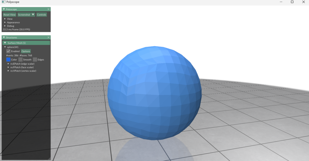
Once the project has been set up, we can begin to test and run our introduction.cu file. If you were to run it, you should get an output of a 3D sphere.
This means the project set up has been successful, we can now begin learning RXMesh.
RXMesh basic workflow
RXMesh provides custom data structures and functions to handle various low-level computational tasks that would otherwise require low-level implementation. Let’s explore the fundamentals of how this workflow operates.
The above is a slightly simplified version of what a for_each computation program would look like using RXMesh. for_each involves accessing every mesh element of a specific type (vertex, edge, or face) and performing some process on/with it.
In the code example above, the computation adjusts the green component of the vertex’s color based on the vertex’s Y coordinate in 3D space.
But how do we comprehend this code? We will look at it line by line:
The above line declares the RXMeshStatic object. Static here stands for a static mesh (one whose connectivity remains constant for the duration of the program’s runtime). Using the RXMesh’s Input directory, we can use some meshes that come with it. In this case, we pass in the dragon.obj file, which holds the mesh data for a dragon.
auto polyscope_mesh = rx.get_polyscope_mesh();
This line returns the data needed for Polyscope to display the mesh along with any attribute content we add to it for visualization.
auto vertex_pos = *rx.get_input_vertex_coordinates();
This line is a special function that directly gives us the coordinates of the input mesh.
auto vertex_color = *rx.add_vertex_attribute<float>("vColor", 3);
This line gives vertex attributes called “vColor”. Attributes are simply data that lives on top of vertices, edges, or faces. To learn more about how to handle attributes in RXMesh, check out this. In this case, we associate three float-point numbers to each vertex in the mesh.
The above lines represent a lambda function that is utilized by the for_each computation. In this case, for_each_vertex accesses each of the vertices of the mesh associated with our dragon. We pass in the arguments:
rxmesh::DEVICE – to let RXMesh know this is happening on the device i.e., the GPU.
[vertex_color, vertex_pos] – represents the data we are passing to the function.
(const rxmesh::VertexHandle vh) – is the handle that is used in any RXMesh computation. A handle allows us to access data associated to individual geometric elements. In this case, we have a handle that allows us to access each vertex in the mesh.
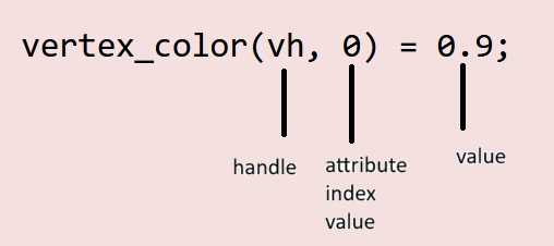
These 3 lines bring together a lot of the declarations made earlier. Through the kernel, we are accessing the attribute data we defined before. Since we need to know which vertex we are accessing its color, we pass in vh as the first argument. Since a vertex has three components (standing for RGB), we also need to pass which index in the attribute’s vector (you can think of it as a 1D array too) we are accessing. Hence vertex_color(vh, 0) = 0.9; which stands for “in the vertex color associated with the handle vh (which for the kernel represents a specific vertex on the mesh), the value of the first component is 0.9”. Note that this “first component” represents red for us.
What about vertex_color(vh, 1) = vertex_pos(vh, 1)? This line, similar to the previous one, is accessing the second component associated with the color, in the vertex the handle is associated with.
But what is on the right-hand side? We are accessing vertex_pos (our coordinates of each vertex in the mesh) and we are accessing it the same way we access our color. In this case, the line is telling us that we are accessing the 2nd positional coordinate (y coordinate) associated with our vertex (that our handle gives to the kernel).
vertex_color.move(rxmesh::DEVICE, rxmesh::HOST);
This line moves the attribute data from the GPU to the CPU.
This line uses Polyscope to add a “quantity” to Polyscope’s visualization of the mesh. In this case, when we add the VertexColorQuantity and pass vertex_color, Polyscope will now visualize the per-vertex color information we calculated in the lambda function.
polyscope::show();
We finally render the entire mesh with our added quantities using the show() function from Polyscope.
Throughout this basic workflow, you may have noticed it works similarly to any other program where we receive some input data, perform some processing, and then render/output it in some form.
More specifically, we use RXMesh to read that data, set up our attributes, and then pass that into a kernel to perform some processing. Once we move that data from the device to the host, we can either perform further processing or render it using Polyscope.
It is important to look at the kernel as computing per geometric element. This means we only need to think of computation on a single mesh element of a certain type (i.e., vertex, edge, or face) since RXMesh then takes this computation and runs it in parallel on all mesh elements of that type.
Writing kernels for queries
While our basic workflow covers how to perform for_each operation using the GPU, we may often require geometric connectivity information for different geometry processing tasks. To do that, RXMesh implements various query operations. To understand the different types of queries, check out this part of the README.
We can say there are two parts to run a query.
The first part consists of creating the launchbox for the query, which defines the threads and (shared) memory allocated for the process along with calling the function from the host to run on the device.
The second part consists of actually defining what the kernel looks like.
We will look at these one by one.
Here’s an example of how a launchbox is created and used for a process where we want to find all the vertex normals:
Notice how, in replacing the for_each part of our basic workflow, we instead declare the launchbox and call our function compute_vertex_normal (which we will look at next) from our main function.
We must also define the kernel which will run on the device.
template <typename T, uint32_t blockThreads>
__global__ static void compute_vertex_normal(const rxmesh::Context      context,
rxmesh::VertexAttribute<T> coords,
rxmesh::VertexAttribute<T> normals)
{


    auto vn_lambda = [&](FaceHandle face_id, VertexIterator& fv){
        // get the face's three vertices coordinates
        glm::fvec3 c0(coords(fv[0], 0), coords(fv[0], 1), coords(fv[0], 2));
        glm::fvec3 c1(coords(fv[1], 0), coords(fv[1], 1), coords(fv[1], 2));
        glm::fvec3 c2(coords(fv[2], 0), coords(fv[2], 1), coords(fv[2], 2));

        // compute the face normal
        glm::fvec3 n = cross(c1 - c0, c2 - c0);

        // the three edges length
        glm::fvec3 l(glm::distance2(c0, c1),
                     glm::distance2(c1, c2),
                     glm::distance2(c2, c0));

        // add the face's normal to its vertices
        for (uint32_t v = 0; v < 3; ++v) {
// for every vertex in this face
            for (uint32_t i = 0; i < 3; ++i) {
// for the vertex 3 coordinates
                atomicAdd(&normals(fv[v], i), n[i] / (l[v] + l[(v + 2) % 3]));
            }
        }
    };

    auto block = cooperative_groups::this_thread_block();

    Query<blockThreads> query(context);
    ShmemAllocator      shrd_alloc;
    query.dispatch<Op::FV>(block, shrd_alloc, vn_lambda);
}
A few things to note about our kernel
We pass in a few arguments to our kernel.
We pass the context which allows RXMesh to access the data structures on the device.
We pass in the coordinates of each vertex as a VertexAttribute
We pass in the normals of each vertex as an attribute. Here, we accumulate the face’s normal on its three vertices.
The function that performs the processing is a lambda function. It takes in the handles and iterators as arguments. The type of the argument will depend on what type of query is used. In this case, since it is an FV query, we have access to the current face(face_id) the thread is acting on as well as the vertices of that face using fv.
Notice how within our lambda function, we do the same as before with our for_each operation, i.e., accessing the data we need using the attribute handle and processing it for some output for our attribute.
Outside our lambda function, notice how we need to set some things up with regards to memory and the type of query. After that, we call the lambda function to make it run using query.dispatch
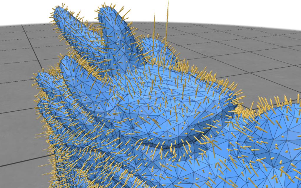
Visualizing face normals
Now that we’ve learnt all the pieces required to do some interesting calculations using RXMesh, let’s try a new one out.
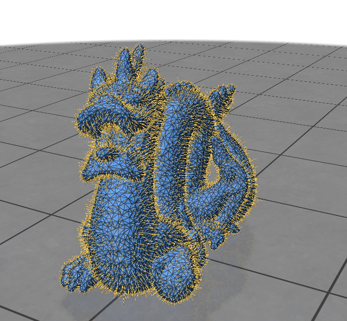
Try to visualize the face normals of a given mesh. This would mean obtaining an output like this for the dragon mesh given in the repository:
Here’s how to calculate the face normals of a mesh:
Take a vertex. Calculate two vectors that are formed by subtracting the selected vertex from the other two vertices.
Take the cross product of the two vectors.
The vector obtained from the cross product is the normal of the face.
Now try to perform the calculation above. We can do this for each face using the vertices it is connected to.
All the information above should give you the ability to implement this yourself. If required, the solution is given below.
The kernel that runs on the device:
template <typename T, uint32_t blockThreads>
global static void compute_face_normal(
const rxmesh::Context context,
rxmesh::VertexAttribute coords, // input
rxmesh::FaceAttribute normals) // output
{
auto vn_lambda = [&](FaceHandle face_id, VertexIterator& fv) {
    // get the face's three vertices coordinates

    glm::fvec3 c0(coords(fv[0], 0), coords(fv[0], 1), coords(fv[0], 2));
    glm::fvec3 c1(coords(fv[1], 0), coords(fv[1], 1), coords(fv[1], 2));
    glm::fvec3 c2(coords(fv[2], 0), coords(fv[2], 1), coords(fv[2], 2));

    // compute the face normal
    glm::fvec3 n = cross(c1 - c0, c2 - c0);
    normals(face_id, 0) = n[0];
    normals(face_id, 1) = n[1];
    normals(face_id, 2) = n[2];
};

auto block = cooperative_groups::this_thread_block();
Query<blockThreads> query(context);
ShmemAllocator shrd_alloc;
query.dispatch<Op::FV>(block, shrd_alloc, vn_lambda);

}
Color a vertex depending on how many vertices it is connected to.
Test the above on different meshes and see the results. You can access different kinds of mesh files from the “Input” folder in the RXMesh repo and add your own meshes if you’d like.
By the end of this, you should be able to do the following:
Know how to create new subdirectories in the RXMesh Fork
Know how to create your own for_each computations on the mesh
Know how to create your own queries
Be able to perform some basic geometric analyses’ using RXMesh queries
This blog was written by Sachin Kishan during the SGI 2024 Fellowship as one of the outcomes of a two week project under the mentorship of Ahmed Mahmoud and support of Supriya Gadi Patil as teaching assistant.
I’m Sergius Nyah, a pre-final year Computer Science student at University of Buea, Cameroon. ( If you’re familiar with Banff, Alberta, Canada, you should appreciate the stunning scenery of Buea as well.) I first encountered the term “Geometry” in 9th grade (Form 4), in our Math class, and had no idea by then of its true significance.
Late 2022 was a peculiar period for me. My very special friend and past SGI fellow introduced me to the Summer Geometry Initiative. From then my immediate reaction was to research on it, connect with past fellows via LinkedIn, and bookmark it for applications, with only very little knowledge on the topic itself, apart from math theories and coding knowledge acquired in the classroom.
What the SGI means to me.
Permit me re-define what the SGI is in two ways. First from the perspective of a prospective applicant, and second as a fellow 🙂
As an applicant, the SGI is a six-week paid summer research program introducing undergraduate and graduate students to the field of geometry processing.
For current or former fellows, the SGI is an intense period of reading research papers engaged around Geometry, listening to talks you may find interesting, learning math for those without a strong math background, acquiring coding skills for students new to programming, and using this knowledge to solve problems on a daily basis, all while learning from Rock-star professors and brilliant students from around the world. Makes sense ? (Without forgetting the generous stipend 🙌🏿 and swag pack 🙂
My Experience so far!
July 8th was the much-anticipated day. That serene evening, we were officially welcomed to the Summer Geometry Initiative 2024 by Professor Justin Solomon, SGI chairman and organizer. My heart boggled with joy as I finally met him and other fellows (now friends 🙂 like Megan Grosse, Aniket Rajnish, Johan Azambou, Charuka Bandra, and a few others, with whom I had been chatting with. Proff Justin opened the floor for the tutorial week and provided us with a brief overview of what the upcoming weeks would entail.
The Tutorial week was a perfect blend of fun and fast-paced learning. Right after Prof. Justin’s welcoming, we had our first tutor for Day 1 — the “Marvelous” Professor Oded Stein, a Computer Science professor from the University of Southern California and tutorial week chair for SGI ’24. Prof. Oded introduced us to Geometry Processing (GP) and its significance to various groups, from artists to programmers. He also taught on surfaces, meshes, explaining how to represent them using triangles and faces, and how to store them using object-lists and face-lists. Additionally, we explored the different types of curvatures (normal curvature, Mean curvature, Principle curvature, Gaussian curvature, and Discrete Gaussian curvature). Next was a session on visualizing 3D data, led by Qingnan Zhou, an Engineer from Adobe Research.
On Day 2, led by Richard Liu, PhD student at the University of Chicago, we focused on parameterization and its vast potential in related fields such as computer graphics. Right after launch/exercise/siesta/rest/fun/ break 😊, we welcomed Dale Decatur, still a PhD student at the University of Chicago, who shared valuable insights on the technical know-how that would be beneficial during our research weeks.
Silvia Sellán, a pre-postdoctoral fellow at MIT and an incoming Professor at the University of Columbia, was in charge of Day 3. She spoke on the various methods of representing shapes, exploring the advantages and disadvantages of each method with regards to computer resources such as memory and processing power. The day ended with an interactive presentation from Towaki Takikawa, a PhD student at the University of Toronto, who focused on Neural Fields.
Day 4, led by Derek Liu, a research scientist at Roblox, taught on Mesh Simplification and Level of Detail (LOD). He mentioned that there are three types of Mesh simplifications: Static Simplification, which includes creating separate level of detail (LOD) models before rendering, DynamicSimplification which provides a continuous spectrum of LOD models instead of a few discrete models, and View-DependentSimplification where the level of detail varies within the model. Later on, Eris Zhang – a Stanford PhD student delved deeper into more technical concepts that proved to be highly beneficial for both the day’s exercises and the upcoming research weeks.
On Day 5, Dr. Nicholas Sharp, a research scientist at NVIDIA and inventor of Polyscope, a highly beneficial software tool in the GP community, led the session, marking the conclusion of the tutorial week. Dr. Nick discussed good and bad surface meshes (data), and the process of remeshing ( which involves turning a bad mesh into a good one). Additionally, we hosted a complementary session featuring guest speaker Zachary Ferguson, a postdoc researcher at MIT, who discussed handling floating points in collision detection.
In summary, Research Week 1 was led by Dr. Nicholas Sharp, research scientist at NVIDIA (A.K.A The G.O.A.T – Greatest Of All Time 🙌🏿). Our research topic focused on how “Well” various surfaces can approximate deforming meshes. I learned about chamfer distances, the Gromov-Hausdorff distance (the largest of all minimum (Chamfer) distances along two curves), and the polyline algorithm. We concluded the week with our first group article on How to Match the Wiggleness of Two Shapes, published by Artur Bogayo.
During Research Week 2, my team mates — Nicolas Pigadas and Champ – and I, led by Dr. Karthik Gopinath from Harvard Medical School explored a nouvel way of parcellating cortical meshes as 2D segments via the process of Pseudo-Rendering.
To conclude this post, I’d like to share the biggest lessons I’ve learned from the first four weeks of the SGI.
Lesson 1: Always request a helping hand when you can’t figure things out. There’s no benefit struggling with a problem when others are just a step away. Don’t hesitate to ask for help!
Lesson 2: Learn to adapt fast to changes. The SGI, like life in general, is fast-paced. Adapting to new research projects and working with different mentors and colleagues is a valuable skill that will significantly boost productivity.
Lesson 3: Cultivate Self-discipline! Learning new concepts takes time. Sitting on that reading table for hours could be tiring, but please, persevere! The juice is definitely worth the squeeze!
Lesson 4: Be transparent with your mentors/supervisors. They may be able to figure things out, but being honest about your situation demonstrates integrity and builds trust. Being honest with what went wrong is a quality people value in long-term collaborators. Don’t sugarcoat things. Tell them what went wrong. They might bite you, but won’t eat you! 😄
Lesson 5: Do what needs doing, regardless. I started writing this blog many days ago, but only got to finish today due to a weeks-long (ongoing) power outages. And here I am now, in the dim light of a local bar at an odd hour, exposed to thieves and weird stuff (like who knows?). So do what you should do! Excuses might seem valid at the moment, but will totally seem completely irrelevant in the future.
As the SGI winds down, I’m filled with so much gratitude for this once-in-a-lifetime opportunity. I brace myself with resilience, dedication, and an insane collaboration towards the rest of our projects, with a full focus on making the most out of this tremendous initiative I’m blessed to have taken part in. A huge thank you to all my mentors, fellows-turned-friends, and everyone for making this year’s SGI what it already is and soon would be!
CLIP is a system designed to determine which image matches which piece of text in a group of images and texts.
1. How it works:
• Embedding Space: Think of this as a special place where both images and text are transformed into numbers.
• Encoders: CLIP has two parts that do this transformation:
– Image Encoder: This part looks at images and converts them into a set of numbers (called embeddings).
– Text Encoder: This part reads text and also converts it into a set of numbers(embeddings).
2. Training Process:
• Batch: Imagine you have a bunch of images and their corresponding texts in a group(batch).
• Real Pairs: Within this group, some images and texts actually match (like an image of a cat and the word ”cat”).
• Fake Pairs: There are many more possible combinations that don’t match (like an image of a cat and the word ”dog”).
3. Cosine Similarity: This is a way to measure how close two sets of numbers (embeddings) are. Higher similarity means they are more alike.
4. CLIP’s Goal: CLIP tries to make the embeddings of matching images and text (real pairs) as close as possible. At the same time, it tries to make the embeddings of non-matching pairs (fake pairs) as different as possible.
5. Optimization:
• Loss Function: This is a mathematical way to measure how good or bad the current matchings are.
• Symmetric Cross-Entropy Loss: CLIP uses a specific type of loss function that looks at the similarities of both real and fake pairs and adjusts the embeddings to improve the matchings.
In essence, CLIP learns to accurately match images and texts by continuously improving how it transforms them into numbers so that correct matches are close together and incorrect ones are far apart.
After learning CLIP, I chose my data set and got to work:
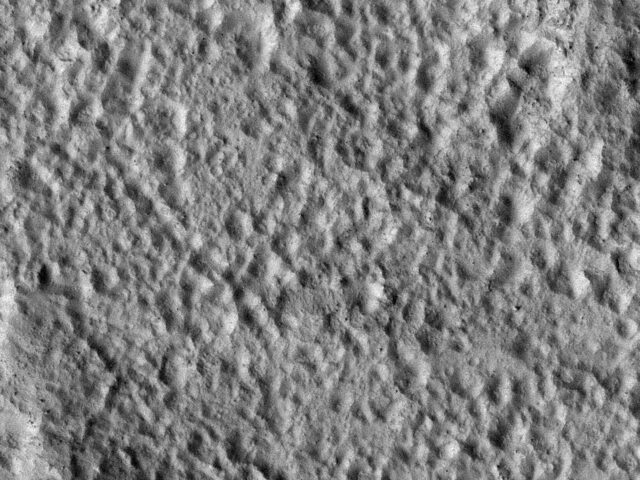
The Describable Textures Dataset (DTD) is an evolving collection of textural images in the wild, annotated with a series of human-centric attributes, inspired by the perceptual properties of textures.
The package contains:
1. Dataset images, train, validation, and test.
2. Ground truth annotations and splits used for evaluation.
3. imdb.mat file, containing a struct holding file names and ground truth labels.
Example images:
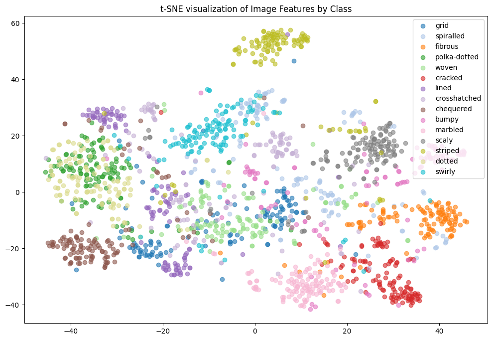
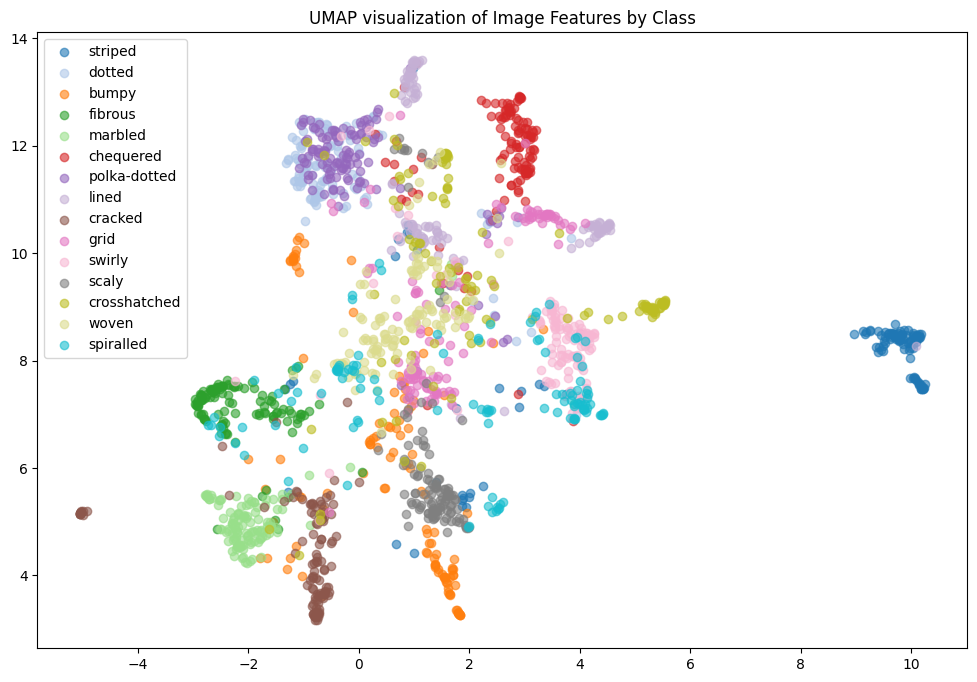
There are 47 texture classes, with 120 images each for a total of 5640 images in this data set. The above shows ‘cobwebbed’, ‘pitted,’ and ‘banded’. I did the t-SNE visualization by class for all the classes but realized this wasn’t very helpful for analysis. It was the same for UMAP. So I decided to sample 15 classes and then visualize:
In the t-SNE for 15 classes, we see that ’polka-dotted’ and ’dotted’ are clustered together. This intuitively makes sense. To further our analysis, we computed the subspace angles between the classes. Many pairs of categories have an angle of 0.0, meaning their feature vectors are very close to each other in the feature space. This suggests that these textures are highly similar or share similar feature representations. For instance:
• crosshatched and striped
• dotted and grid
• dotted and polka-dotted
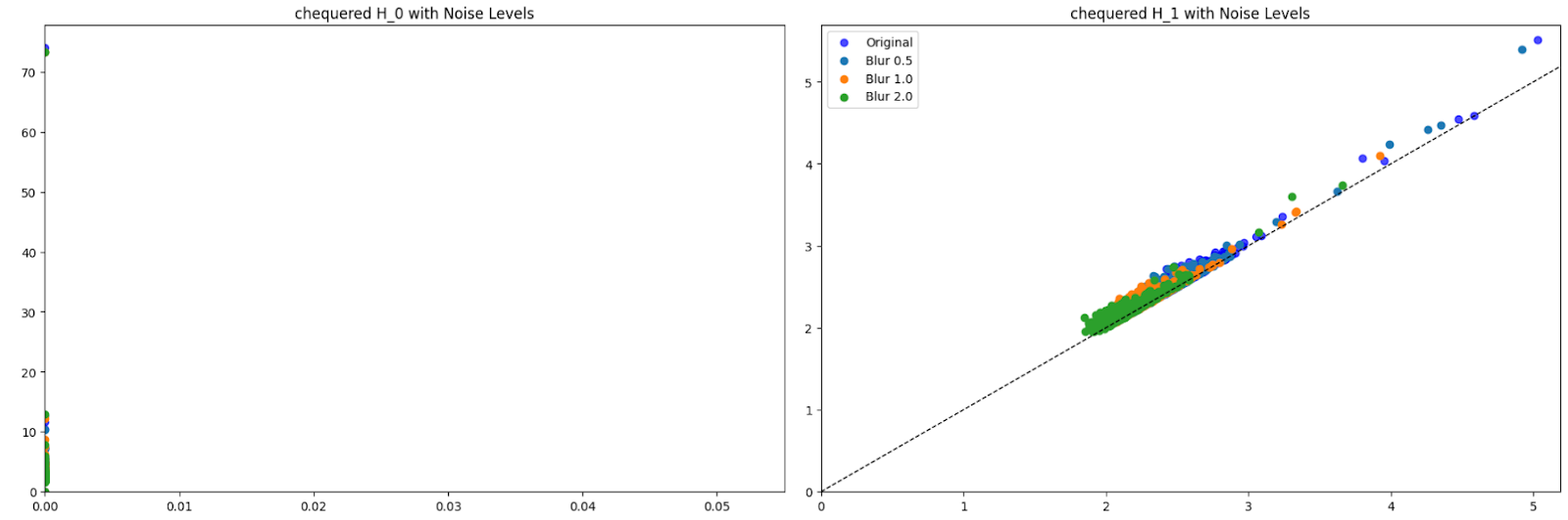
Then came the tda: A persistence diagram summarizes the topological features of a data set across multiple scales. It captures the birth and death of features such as connected components, holes, and voids as the scale of observation changes. In a persistence diagram, each feature is represented as a point in a two-dimensional space, where the x-coordinate corresponds to the “birth” scale and the y-coordinate corresponds to the “death” scale. This visualization helps in understanding the shape and structure of the data, allowing for the identification of significant features that persist across various scales while filtering out noise.
I added 3 levels of noise (0.5, 1.0, 2.0) to the images and then extracted features. I visualized these features on a persistence diagram. Here are some examples of those results. We can see that for H_0 at all noise levels, there is one persistent feature so there is one connected component. The death of this persistent feature varies slightly. H_1 at all noise levels there aren’t any highly persistent features, with most points being around the diagonal. The features in H_1 tend to “clump up together” and die quicker as the noise level goes up.
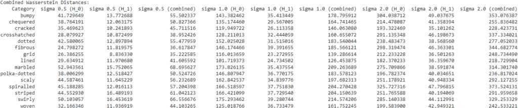
I then computed the distances between the diagrams with no noise and those with noise. Here are some of those results. Unsurprisingly, with greater levels of noise, there is greater distance.
Finally, we wanted to test the robustness of CLIP so we classified images with respect to noise. The goal was to see if the results we saw with respect to the topology of the feature space corresponded to the classification results. These were the classification accuracies:
Hello world! I’m Kimberly Herrera. I was born and raised in LA county but I’m currently in the Bay Area where I’m a senior at UC Berkeley. I study pure math and math education. I applied to SGI because I had previously gotten a taste of topological data analysis this previous summer and I guess I wanted to see other ways in which math and coding ‘mesh.’😎
Tutorial week I’m in California so that meant waking up before 8 am which kinda sucked but I got used to it. I’m also someone who has a hard time learning remotely so I was worried, but thankfully the lecturers were great. I was able to follow along (mostly) while growing interested in the material. I think my favorite lesson was on 2D and 3D shape representations. This wasn’t particularly new to me, having worked with point clouds and cubic splines before, but Silvia was a very engaging speaker. She presented the material in a way that was so digestible. By the end of the week, I hadn’t nearly finished all of the exercises but I made sure to do a few from each lesson so I could be prepared for the coming weeks.
When ranking projects, a lot of the descriptions were just buzzwords for me. I just decided to choose whichever ones had prerequisites I satisfied. I actually got my first choice for my first project, which I chose because it involved tda.
Project 1: In our first meeting, we introduced ourselves and our background in topology and machine learning. Our mentor then told us the goals of the project, which I made sure to write down. We then immediately went to work. I started by investigating the neural network CLIP we would be using for image classification. I also researched what feature spaces were. This project went on for 2 weeks and we only met as a team like 4 times, although we did consistently communicate through Slack. However, it did feel like “here’s what you need to do, now go do it,” which was fine with me. I was proud of my work on this project, I completed everything I needed to do and was able to communicate my findings in our meetings.
Project 2: This project is so different from the last. This mentor started by presenting slides on the background and goals for the project. I also noticed that the TA was more active, I think because they are a graduate student of the mentor. We also meet every day in the morning and have a follow-up meeting to discuss our work for the day. That being said, I don’t think I’ve completed as much work on this project thanks to errors with running the code. Hopefully, more progress will be made in the coming days.
In comparison to previous research: SGI has been a bit different from the REU I did last summer. Having a tutorial week and guest lectures is the same, but here we do multiple mini projects instead of deep diving into one sole project. This of course leads to engaging with different kinds of people and different work ethics. Last summer I was working 9-5 while this time it depends on the project and the mentor. Another big difference of course is how coding/cs heavy this project is compared to my previous project. Previously, we did a deeper dive into the mathematical background (since it was a math REU) and the coding was done to inform the math. Now it feels like the math is learned in order to inform the CS/Machine learning.
Overall, I am having a good time and am excited for the next two weeks 🙂