Author: Ehsan Shams (Alexandria University, EG)
Project Mentor: Justin Solomon (MIT, USA)
Volunteers: Biruk Ambaw (Université Paris-Saclay, Fr), Andrew Rodriguez (Georgia Institute of Technology, USA), and Josh Vekhter ( UT Austin, USA)
Acknowledgments. Sincere thanks to Professor Justin Solomon for his invaluable guidance throughout this project. His carefully designed questions and coding tasks not only deepened my understanding of core topics in geometry processing in a short amount of time, but also sharpened my coding skills—and ensured my lunch breaks were notably shorter than they might have been otherwise :). I would also like to thank Josh Vekhter, Andrew, and Biruk for their support and valuable feedback to my teammates and me. In addition to the math and codes, Professor Justin and Josh taught me the value of a well-timed joke to lighten the load!
Introduction
Mean Curvature Flow (MCF) is a fundamental geometric evolution partial differential equation (PDE) that describes the motion of a surface \(\mathcal{M}_t \subset \mathbb{R}^3\) under its mean curvature. Each point on the surface moves in the direction of the unit normal vector to the surface with velocity proportional to the mean curvature, leading to a smoothing effect that regularizes the geometry of the surface over time. MCF is widely studied in differential geometry and geometric analysis due to its intrinsic connection to minimal surfaces and its role in shape optimization. In computational applications, MCF is particularly useful in geometry processing (GP), including tasks such as surface fairing, mesh denoising, and feature-preserving smoothing.
The discretization of the MCF PDE consists of both spatial and temporal components. Spatial discretization is well-established, with common techniques such as finite element methods, discrete exterior calculus, and discrete differential geometry effectively approximating the part of the equation that governs the surface’s spatial evolution. In contrast, temporal discretization remains challenging due to stability constraints and accuracy limitations.
Three primary approaches exist for temporal discretization: explicit, implicit, and semi-implicit methods. Explicit methods, like forward Euler, often become unstable with larger time steps. Implicit methods, such as backward Euler, offer stability but at a high computational cost. Semi-implicit methods, like the one introduced by Desbrun et al. (1999), strike a compromise between these two extremes but may still fall short in terms of accuracy and stability. In practice, the temporal discretizations that are commonly employed in the literature are only first-order accurate thus, may not provide the desired level of accuracy and stability we ideally wish for.
The central focus of this project was to derive and implement higher-order temporal discretizations—both explicit and semi-implicit—for MCF on triangular meshes, with the goal to improve the numerical accuracy of the discrete evolution of the surface by reducing truncation errors and better approximating the continuous PDE solution, particularly for larger time steps. By increasing temporal accuracy, we aim to enhance both the fidelity of the simulated flow and the computational efficiency, mitigating the need for excessively small time steps while maintaining stability.
In this article, I externalize my internal exploratory journey and insights gained during my last SGI research week under the guidance of my mentors. The article begins with an introduction to MCF and its significance in GP, followed by a brief discussion on the process of discretization followed by the derivation of spatial discretization via finite element methods and first-order accurate temporal discretization via finite difference methods for MCF. A theoretical comparison of the methods in question is then provided, highlighting their pros and cons. Finally, we derive the second-order accurate temporal discretization of MCF, in both, the explicit, and semi-implicit schemes. Empirical validations of theoretical results are also presented, along with a humorous fail. The goal here is on exposition, rather than taking the shortest path.
Understanding Mean Curvature Flow in \(\mathbb{R}^3 \)
Formal Definition
Let \(M_t \subset \mathbb{R}^3\) represent a family of smoothly embedded surfaces parameterized by time \(t\). The surface at time \(t\) can be described by a smooth mapping:
\[ X(\mathbf{u}, t) : U \times [0, T) \rightarrow \mathbb{R}^3 \]
Here:
- \(U\) is an open set in \(\mathbb{R}^2\) representing the parameter space of the surface, with local coordinates \( \mathbf{u} = (u_1, u_2)\).
- \([0,T) \) represents time, where \(T\) is the time until which the flow is considered.
- \(X(\mathbf{u}, t)\) is the position vector of a point on the surface in \(\mathbb{R}^3\) at time \(t\), and can be explicitly written as: \[ X(\mathbf{u},t) = \begin{pmatrix} X_1(\mathbf{u},t) \\ X_2(\mathbf{u},t) \\ X_3(\mathbf{u},t) \end{pmatrix} \] and \(X_1(\mathbf{u},t), X_2(\mathbf{u},t), X_3(\mathbf{u},t)\) are the coordinate functions that determine the \(x, y,\) and \(z\) components of the position vector in \( \mathbb{R}^3\)
The mean curvature flow is then dictated by the following partial differential equation:
\[ \frac{\partial X}{\partial t}(\mathbf{u}, t) = – H(\mathbf{u}, t) \mathbf{n}(\mathbf{u}, t) =\Delta X(\mathbf{u}, t)\]
Where:
- \(\frac{\partial X}{\partial t}(\mathbf{u}, t)\) is the velocity of the surface at the point \(X(\mathbf{u}, t)\).
- \(H(\mathbf{u}, t)\) is the mean curvature at the point \(X(\mathbf{u}, t)\).
- \(\mathbf{n}(\mathbf{u}, t)\) is the unit normal vector at the point \(X(\mathbf{u}, t)\), pointing outward or inward. It indicates the direction in which the surface will move during the flow.
- \( \Delta \) is the Laplace-Beltrami operator associated with the surface \(M_t\).
Abuse of Notation. For simplicity, any operator \( \phi (\mathbf{u},t) \) at a point parameterized by \( (\mathbf{u},t))\) will be referred to simply as \( \phi \) in this article. The Laplace-Beltrami operator, might sometimes be referred to as the Laplacian depending on my mood.
Mean Curvature \(H\):
The mean curvature \( H\) at a point is defined as the average of the principal curvatures \( k_1 \) and \( k_2 \) at that point on the surface: \[ H= \frac{1}{2} (k_1 + k_2) \]
Where \(k_1\) and \(k_2\) are the eigenvalues of the second fundamental form of the surface. These principal curvatures measure the maximum and minimum bending of the surface in orthogonal directions at this particular point in question.
Alternative Expressions for \( H \):
- Divergence of the Normal Vector Field: \(H\) can be expressed as the negative half of the divergence of the unit normal vector field \(\mathbf{n}\) on the surface: \( H= – \frac{1}{2} div ((\mathbf{n})) \).
- Trace of the Shape Operator: In addition, \(H\) can be written as the trace of the shape operator (or Weingarten map) associated with the surface. This representation connects the mean curvature to the linear transformation that describes how the surface bends.
Why Study MCF?
Understanding MCF begins with a simple question: what happens when a surface evolves according to its own curvature? In practice, this flow helps smooth surfaces over time, driving them toward more regular shapes. This process is especially intriguing because it captures essential properties of geometric evolution without external forces, relying solely on the surface’s own shape.
A fundamental result by Huisken in 1984 in his paper titled “Flow by Mean Curvature of Convex Surfaces into Spheres” provides deep insight into this phenomenon. Huisken studied the evolution of a special type of hypersurfaces under MCF, and proved that any strictly convex smooth hypersurface, under MCF, evolves into a sphere before collapsing to a point in a finite, self-similar manner in a finite time. His work highlights how MCF transforms surfaces, regularizing their shape as they shrink and demonstrating the flow’s inherent tendency to round out irregularities. In mathematics, it is common practice to first test an idea or prove a theorem in simple and nice settings (such as convex compact spaces) before attempting to test/generalize to more abstract spaces.
While the general theory of MCF applies to a wide range of surfaces, it is particularly insightful to consider how a sphere—a familiar, symmetric object—shrinks under the flow. The sphere offers a clean, intuitive example where the underlying mathematics remains manageable, yet it showcases the essential features of MCF, such as shrinking to a point while maintaining symmetry. This serves as an ideal starting point for understanding more complex behaviors in less regular surfaces, grounded in the theoretical framework established by Huisken’s work.
Example: Shrinking Sphere Under MCF
Consider a sphere of radius \(R(t)\) at time \(t\). Under MCF, the sphere’s surface shrinks over time. We want to find how the volume of the sphere changes as it evolves under this flow.
For a sphere of radius \(R(t)\), the mean curvature \(H\) is given by: \( H=\frac{2}{R(t)}\), and the normal vector \(\mathbf{n}\) points radially inward, so: \(\mathbf{n}=\frac{−X}{R(t)}\)
Substituting these in the MCF equation: \( \frac{\partial X}{\partial t}=\frac{-2}{R(t)} \frac{-X}{R(t)}=\frac{2X}{R^2(t)}\)
To determine how the radius \(R(t)\) changes over time, observe that each point on the surface \(X\) can be written as: \(X=R(t) \mathbf{u}\) where \(\mathbf{u}\) is a unit vector in the direction of \(X\). Thus, \( \frac{\partial X}{\partial t} = \frac{\partial (R(t) \mathbf{u})}{\partial t} = \frac{2\mathbf{u}}{R(t)} \), which simplifies to \( \mathbf{u}\frac{dR(t)}{dt}= \frac{2 \mathbf{u}}{R(t)}\) so \(\frac{dR(t)}{dt}= \frac{2 }{R(t)} \).
To solve for \( R(t) \), we separate the variables and integrate \(\int R(t) \, dR(t) = \int 2 \, dt \) which gives \(\frac{R^2(t)}{2} = 2t + C \), where \( C \) is the constant of integration. Solving for \( R(t) \) gives \( R(t) = \sqrt{4t + C’} \) where \( C’ = 2C \). If we consider the initial condition \( R(0) = R_0 \), then \( R_0^2 = C’ \), and hence: \(R(t) = \sqrt{R_0^2 – 4t} \)
Volume Shrinkage:
The volume \( V(t) \) of the sphere at time \( t \) is \( V(t) = \frac{4}{3} \pi R^3(t) \). As the sphere shrinks over time, the volume decreases according to the following equation: \( V(t) = \frac{4}{3} \pi \left(R_0^2 – 4t \right)^{3/2} \), and it continues to shrink until \( t = \frac{R_0^2}{4} \), at which point the radius reaches zero and the sphere vanishes.
The accompanying animation illustrates the shrinking process, showing how both the radius and volume decrease over time under the influence of MCF until the sphere vanishes. The MCF drives the surface points of the sphere inward in the direction of the inward normals, leading to a uniform shrinking process. For a perfectly symmetric object like a sphere, the shrinking occurs uniformly, preserving the spherical shape until the radius reduces to zero.
The shrinking radius is computed via the derived formula above, \( R(t)= \sqrt{R_0^2 – 4t} \), and the shrinking becomes faster as time progress. The plots that are displayed at the end show the relation between \( R(t) \) and \( V(t) \) over time.
Since computer machines operate in a discrete, digital environment, and GP is inherently computational, continuous geometric surfaces must be represented in a form that computer machines can process. This form is typically a mesh, a discrete approximation of a surface composed of vertices, edges, and faces, and given that MCF is intrinsically a continuous model described by a PDE in space and time, directly applying it to meshes necessitates the discretization of its continuous operators (the Laplacian and time derivatives) as well.
Discretizing MCF
As implied by the above paragraph, discretization is the process of transforming a continuous mathematical model \(\mathcal{M}\), which is defined over a continuous domain \(\Omega \subset \mathbb{R}^n\) and governed by continuous variables \(u(x)\) and operators \(\mathcal{L}\), into a discrete model \(\mathcal{M}_h\) suitable for computational analysis. This involves:
- Replacing the continuous domain \(\Omega\) with a finite set of discrete points or elements \(\Omega_h = {x_i}_{i=1}^N\).
- Approximating continuous functions \(u(x)\) by discrete counterparts \(u_h(x_i)\).
- Substituting continuous operators \(\mathcal{L}\) with discrete analogs \(\mathcal{L}_h\).
The goal is to ensure that the discrete model \(\mathcal{M}_h\) preserves key properties such as consistency, stability, and convergence, so that \(\mathcal{M}_h\) faithfully reflects the behavior of the continuous model \(\mathcal{M}\) as the discretization is refined, i.e., as \(h \rightarrow 0\).
While many continuous models can be discretized, the accuracy and efficiency of the approximation depend on the chosen discretization technique and its implementation. Common discretization techniques include: Finite difference methods (FDM), finite element methods (FEM), finite volume methods (FVM), and spectral methods.
Discretizing the MCF model can be systematically divided into two main components: spatial discretization and temporal discretization. In this article, we employ the FEM for spatial discretization and the FDM for temporal discretization.
Spatial Discretization via FEM
Spatial discretization involves representing the continuous spatial domain of the model as a mesh and approximating differential operators—primarily the Laplacian, and also gradient and divergence as quantities at the discrete mesh in question.
Assume the surface in question is discretized into a mesh which consists of a collection of triangular elements \(\{T_i\}\) with vertices \(v_j\). The first step to approximate the Laplace-Beltrami operator is to define basis functions \(\{\phi_j\}\) associated with the vertices and defined over \(T_i\). These are often linear or piecewise linear functions, \(\phi_j\) takes the value 1 at vertex \(v_j\) and 0 at all other vertices. These basis functions form a set that allows any function \(X\) on the surface to be approximated as a linear combination of them \( X≈ \sum_j X_j \phi_j\), where \(\mathbf{X_j}=\mathbf{X(v_j)}\) represents the value of the position function at vertex \(v_j\).
Next, we compute the gradient of each basis function within each triangle, which will be constant over the triangle because the functions are linear. The Laplacian operator, which in continuous terms is the divergence of the gradient, is discretized by integrating the product of the gradients of the basis functions over the surface. This leads to the construction of the stiffness matrix \(\mathbf{L}\), where each entry \( \mathbf{L_{ij}}\) is derived from the inner products of the gradients of the basis functions \(\phi_i\) and \(\phi_j\) ( \( \nabla \phi_i\) and \(\nabla \phi_j\)), weighted by the cotangent of the angles opposite the edge connecting vertices \(v_i\), and \(v_j\). The diagonal entries \(\mathbf{L_{ii}}\) sum the contributions from all adjacent vertices.
More precisely, for two vertices \(v_i\) and \(v_j\) connected by an edge, the stiffness matrix \(\mathbf{L}\) is computed using the following integral:
\[ \mathbf{L_{ij}}=\int_{\sigma} \nabla \phi_i \cdot \nabla \phi_j dA\]
where \(\sigma\) is the surface, and \(dA\) is the area element.
For a piecewise linear basis function on a triangular mesh, those gradients in question are constant within each triangle, so the integral simplifies to the sum over the triangles \(T_k\) that include the edge connecting \(v_i\) and \(v_j\):
\[ \mathbf{L_{ij}}= \sum_{T_k \in N(v_i,v_j)} (\nabla \phi_i \cdot \nabla \phi_j ) \text{Area} (T_k) \]
Where \( N(v_i,v_j)\) denotes the set of triangles sharing the edge between \(v_i\) and \(v_j\). Now the inner product \(\nabla \phi_i \cdot \nabla \phi_j\) can be computed using the cotangent formula
\[\nabla \phi_i \cdot \nabla \phi_j = \frac{-1}{2 \text{Area}(T_k)}(\cot{\alpha_{ij}}+\cot{\beta_{ij}}) \]
Thus, the entries \( \mathbf{L_{ij}} \) are:
\[\mathbf{L_{ij}}= – \frac{1}{2} (\cot{\alpha_{ij}}+\cot{\beta_{ij}}) \]
Finally the diangonal enteries \(\mathbf{L_{ii}}\) sum the contributions from all the adjacent verticies:
\[\mathbf{L_{ii}}=\sum_{i \neq j} \mathbf{L_{ij}} = \sum_{i \neq j} \frac{1}{2} (\cot{\alpha_{ij}}+\cot{\beta_{ij}})\]
To balance the discretization, we also need the mass matrix \(\mathbf{M}\), which arises from integrating the basis functions themselves. Formally, the entries of the mass matrix \(\mathbf{M}\) are given by:
\[ \mathbf{M_{ij}} = \int_{\sigma} \phi_i \phi_j dA\]
In simple cases1, the mass matrix is typically diagonal, with each entry written as:
\[ \mathbf{M}_{ii} = \frac{1}{3} \sum_{T \ni v_i} \text{Area}(T),\]
where the sum is over all triangles \(T\) that share the vertex \((v_i).\)
The final discretized Laplace-Beltrami operator is represented by the generalized eigenvalue problem \(\mathbf{L}X = \lambda \mathbf{M} X\), where \(\mathbf{L}\) encodes the differential operator and \( \mathbf{M}\) ensures that the discretization respects the geometry of the mesh.
Both matrices (the mass matrix \( \mathbf{M}\) and the stiffness matrix \( \mathbf{L}\)) are positive semi-definite, and sparse.
Intuitively,
- The stiffness matrix \(\mathbf{L}\) captures the geometric and differential properties of the surface. It represents how the curvature is distributed over the mesh by measuring how the gradients of the basis functions (associated with each vertex) interact with each other. The entries of this matrix are weighted by the angles in the triangles, which essentially encode how “stiff” or “resistant” the mesh is to deformation. In other words, it determines how much the shape of the surface resists change when forces (like curvature flow) are applied.
- The mass matrix \(\mathbf{M}\) accounts for the distribution of area or “mass” over the surface. It ensures that the discretization respects the surface’s geometry by distributing weight across the vertices according to the areas of the surrounding triangles. This matrix is often diagonal, with each entry corresponding to the area associated with a vertex, making sure that the mesh’s physical properties, like area and volume, are properly balanced in computations.
Solving the general eignvalue problem, we reach the following approximation of the Laplacian: \(\Delta \approx \mathbf{M}^{-1} \mathbf{L}\).
Remark: In discretizing the Laplacian operator, several other approaches can be employed too such as divided difference, higher-order elements, discrete exterior calculus,..etc. In any case, no discretization approach of the Laplacian could keep every natural property of its ideal continuous form.
Temporal Discretization via FDM
Temporal discretization refers to the approximation of the time-dependent aspects of the MCF model (the time derivative \(\frac{\partial X}{\partial t}\)). This step is critical for evolving the surface over time according to the mean curvature dynamics. Three common approaches are used for this type of discretization: Explicit methods (e.g. Explicit Euler method), Implicit methods (e.g. Implicit Euler method), and Semi-implicit methods (e.g Desbrun et al. (1999)).
- Explicit Euler Method: This method (also known as forward Euler method) is where the new future positions of the mesh vertices are computed based on the current positions and the mean curvature at those positions. While this method is simple to implement, it may impose stability constraints on the time step size. The discretized vertex update rule is given by:
\[\frac{X^{(k+1)} – X^{(k)}}{\Delta t} = \mathbf{M}^{-1} \mathbf{L} X^{(k)} \]
Rearranging this, we get: \[ X^{(k+1)} = X^{(k)} + \Delta t \mathbf{M}^{-1}\mathbf{L} X^{(k)} \] where \(X^{(k)}\) and \(X^{(k+1)}\) are surface position matrix of the mesh vertices at time steps \(k\) and \(k+1\), respectively. - Implicit Euler Method: Also known as backward Euler, this method involves solving a system of equations at each time step, it might provide greater stability compared to the Explicit Euler method and allow for larger time steps. The discretized vertex update rule is given by: \[ X^{(k+1)} \approx X^{(k)} + \Delta t \mathbf{M}^{-1}\mathbf{L} X^{(k+1)} \] This equation is said to be fully implicit because the Laplacian depends on the vertex positions at the time step one is trying to solve for, making it nonlinear and difficult to solve.
- Desbrun et al.’s Semi-Implicit Method: (Desbrun et al. 1999) proposed a semi-implicit method, which is a compromise between the simplicity of explicit methods and the stability of implicit methods. The idea is to treat the Laplacian and the vertex positions in the following manner: Instead of calculating the Laplacian at the next time step (which makes the equation nonlinear), they compute it at the current time step which simplifies the problem, and the vertex positions are still updated at the next time step. Their discretized vertex update rule is given by: \[ X^{(k+1)} \approx X^{(k)} + \Delta t\mathbf{M^{-1}}(\mathbf{L}X^{(k)} )X^{(k+1)} \] This equation is still implicit in \(X^{(k+1)}\), but the Laplacian is evaluated at the known positions \(X^{(k)}\), making the system linear and easier to solve. The update rule can be re-arranged into: \[X^{(k+1)} \approx (I- \Delta t\mathbf{M^{-1}L}X^{(k)} )^{-1}X^{(k)} \]. This method offers nice stability. However, it is not as accurate as fully implicit methods, because it only approximates the Laplacian based on the current positions. It might smooth the mesh, but not as precisely as solving the full nonlinear system such as the fully-implicit. In addition, it does not generalize to other geometric flows that require more complex handling of nonlinearities.
- Adaptive Time Stepping: This approach adjusts the time step size dynamically based on the evolution of the surface, allowing for finer resolution during critical changes and coarser resolution during smoother phases. Progyan Das from my team worked on this approach.
Remark. The derivations for the above update rules are tacitly included in the part we derive their second-order forms.
Comparative Analysis and Empirical Validation: Euler Explicit vs. Desbrun et al.’s
- Accuracy
- Euler Explicit Method:
- Order of Accuracy: This method is first-order accurate in time, meaning that the global error in the solution decreases linearly with the time step \(\Delta t\). If the exact solution at time \(t\) is denoted by \(X_{t}\) and the numerical solution by at time \(t_n\) by \(X_{t_n}\), the error \(E_n = X(t_n) \) satisfies\(E_n \approx C \Delta t\), where \(C\) is a constant dependent on the problem. This linear relationship implies that halving the time step approximately halves the error.
- Error Propagation: Errors tend to accumulate more rapidly, especially for larger time steps. Because this method updates the solution based only on information from the current time step so, if the time step \(\Delta t\) is too large, the method may not accurately capture the evolution of the curvature, leading to significant errors that compound over time. The error propagation can be expressed as \(X^{(k+1)}=X^{(k)}+ \Delta t \dot F(X^{(k)})\), where \(F(X^{(k)})\) is the update function. If\(\Delta t\) is too large, the local truncation error, which is \(O(\Delta t^2)\), becomes significant, causing larger cumulative errors.
- Handling of Complex Geometries: Will probably struggle with highly irregular meshes, which is a direct consequence of the above bullet. leading to larger errors in curvature computation.
- Desbrun et al. Semi-Implicit Method:
- Order of Accuracy: This method is also first-order accurate in time because it is essentially a modified backward Euler scheme, where the implicit part is handled for spatial discretization, but the time discretization remains first-order.
- Error Propagation Reduction: The method implicitly handles the curvature of the mesh by solving a linear system at every update, which incorporates more information about the solution at the next time step. This implicit approach effectively reduces errors, and stabilizes the solution especially when larger time steps are used compared to Euler’s explicit method.
- Numerical Diffusion: Moreover, it has a better control over numerical diffusion —a phenomenon where fine details of the mesh are smoothed out excessively—compared to the explicit method, leading to more accurate smoothing. Numerical diffusion can be mathematically described by how the curvature smoothing term affects the higher-order modes of the solution and here is where the implicit nature of the method helps preserve these modes more effectively than Euler’s explicit method.
- Euler Explicit Method:
- Stability
- Euler Explicit Method:
- Conditionally Stable: The stability here depends on the time step size; it requires small time steps to maintain stability.
- CFL Condition: The time step must satisfy the Courant-Friedrichs-Lewy (CFL) condition, which can severely restrict the time step size, especially for fine meshes. The CFL condition constrains the time step to be inversely proportional to the square of the mesh resolution. This means that as the mesh becomes finer, the time step must decrease quadratically, which significantly increases the number of iterations required for convergence.
- Desbrun et al. Semi-Implicit Method:
- Unconditionally Stable: Allows larger time steps without sacrificing stability. This is a key advantage for computational efficiency.
- Robustness: More stable under large deformations or irregular meshes, making it suitable for a broader range of applications than the explicit method.
- Euler Explicit Method:
- Computational Efficiency and Memory Usage
- Euler Explicit Method:
- Efficiency: Simpler to implement and faster per iteration due to direct updates, but requires more iterations for convergence due to the small time steps needed.
- Memory Usage: Lower memory requirements since it does not require solving linear systems.
- Parallelization: Easier to parallelize due to the independence of the update steps.
- Desbrun et al. Semi-Implicit Method:
- Efficiency: More computationally intensive per iteration due to the need to solve linear systems, but fewer iterations may be needed due to larger permissible time steps.
- Memory Usage: Higher memory consumption due to the storage of matrices for linear system solving.
- Parallelization: More challenging to parallelize because of the dependencies introduced by solving the linear system.
- Euler Explicit Method:
- Implementation Complexity
- Euler Explicit Method:
- Complexity: Conceptually simpler and easier to implement. It involves straightforward updates without the need for solving linear systems.
- Dependencies: Minimal dependencies between updates, making it a more accessible method for quick implementations.
- Desbrun et al. Semi-Implicit Method:
- Complexity: More complex to implement due to the need to solve large, sparse linear systems at each time step.
- Dependencies: Involves matrix assembly and inversion, which can introduce additional challenges in implementation.
- Euler Explicit Method:
- Parameter Sensitivity
- Euler Explicit Method:
- Sensitivity: Highly sensitive to time step size. Small changes can significantly affect stability and accuracy.
- Desbrun et al. Semi-Implicit Method:
- Sensitivity: Less sensitive to time step size, allowing for greater flexibility in choosing time steps.
Overall Assessment:
- Euler Explicit Method is advantageous for its simplicity, ease of implementation, and parallelization potential. However, it is limited by stability constraints, accuracy issues, and higher sensitivity to parameter choices.
- Desbrun et al. Semi-Implicit Method offers superior stability, accuracy when compared to the explicit, and reduced numerical diffusion at the cost of increased computational complexity and memory usage. It is better suited for applications requiring robust and accurate smoothing, particularly in the context of complex or irregular meshes.
Oh… this felt like eating five horrible McDonald’s cheeseburgers. 🍔🍔🍔🍔🍔 Right? So, let’s compress this previous analysis into a nice compact table for quick reference.
| Aspect | Euler Explicit Method | Desbrun et al. Semi-Implicit Method |
|---|---|---|
| Accuracy | First-order accurate in time. Higher error accumulation, especially for large time steps. Struggles with complex geometries. | First-order accurate in time. Better error reduction, especially for large time steps. Better control over numerical diffusion. |
| Stability | Conditionally stable. Requires small time steps, dictated by the CFL condition. | Unconditionally stable. Allows larger time steps without sacrificing stability. |
| Computational Efficiency | Simple and fast per iteration. Inefficient for fine meshes due to small time step requirement. | Computationally more expensive due to solving linear systems. Efficient for larger time steps. |
| Memory Usage | Lower memory usage. | Higher memory usage due to storing and solving linear systems. |
| Implementation Complexity | Relatively simple to implement. | More complex due to the need to solve linear systems. |
| Parallelization | Easier to parallelize due to independent updates. | More challenging to parallelize due to solving linear systems. |
| Parameter Sensitivity | Sensitive to time step size (CFL condition). | Less sensitive to time step size, allowing more flexibility. |
| Numerical Diffusion | Higher numerical diffusion, especially for large time steps. | Better control over numerical diffusion, preserving more detail. |
The next experiment aims to empirically illustrate the above tradeoffs in the stability and accuracy aspects presented above for the two methods in question for MCF since the main aim of the project is to come up with an approach to improving the accuracy and stability of MCF applied to triangle meshes by incorporating higher-order derivatives in the time integration process.
Experimental Design:
- Mesh Preparation:
- Target Mesh: Load a 3D mesh model, and store it as the target mesh.
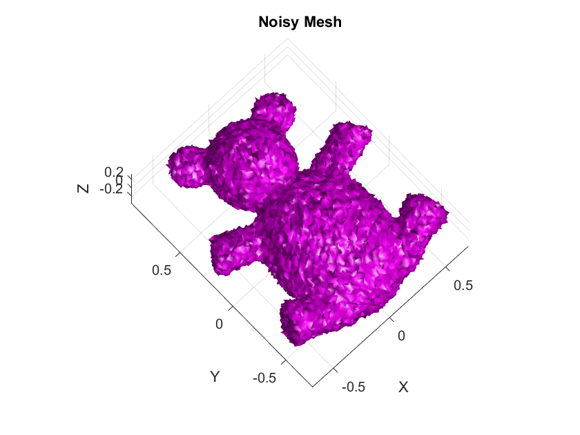
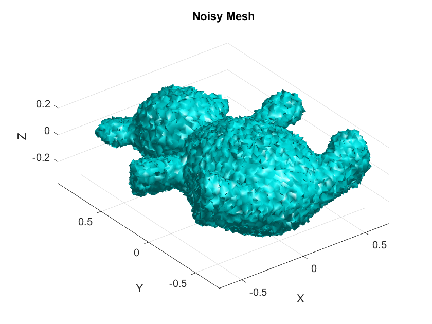
- Noisy Mesh: Add a controlled amount of noise to simulate imperfections to the target mesh and store the output as the noisy mesh.
- Application of MCF Methods:
- Apply each MCF method to the noisy mesh across a series of pre-determined range of time steps. The number of iterations for both methods is fixed (10 iterations) per each time step. Choose the range of the time steps such that it includes very small (those satisfying the CFL condition) to relatively large time steps to allow for a comprehensive analysis of the methods’ behavior under different conditions.
- Data Logging: For each time step, record the following data for each method:
- Error Metric: Frobenius norm of the difference between the smoothed mesh and the original target mesh.
- Stability Metric: the number of maximum \(\Delta t\) where the error stays less than a pre-determined error threshold by the user.
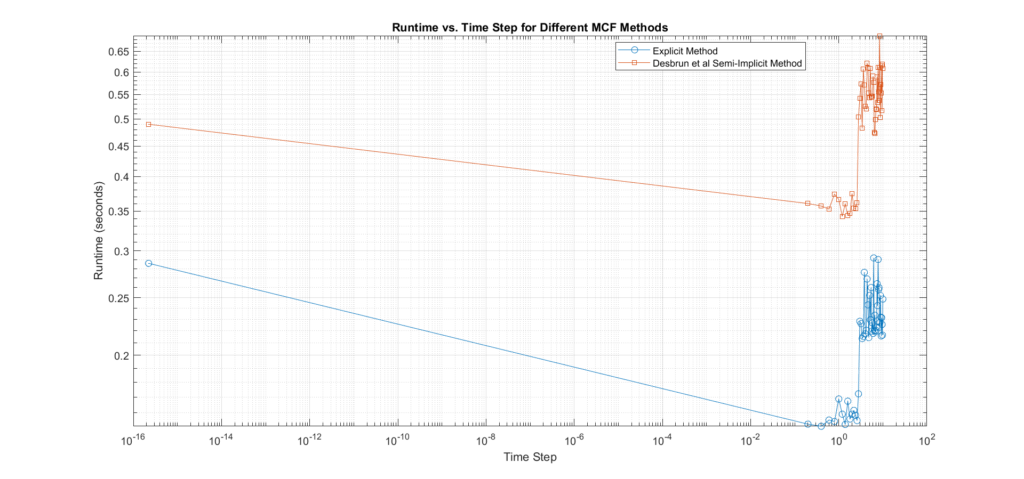
- Computational Time: Time taken for execution.
- Output Plots
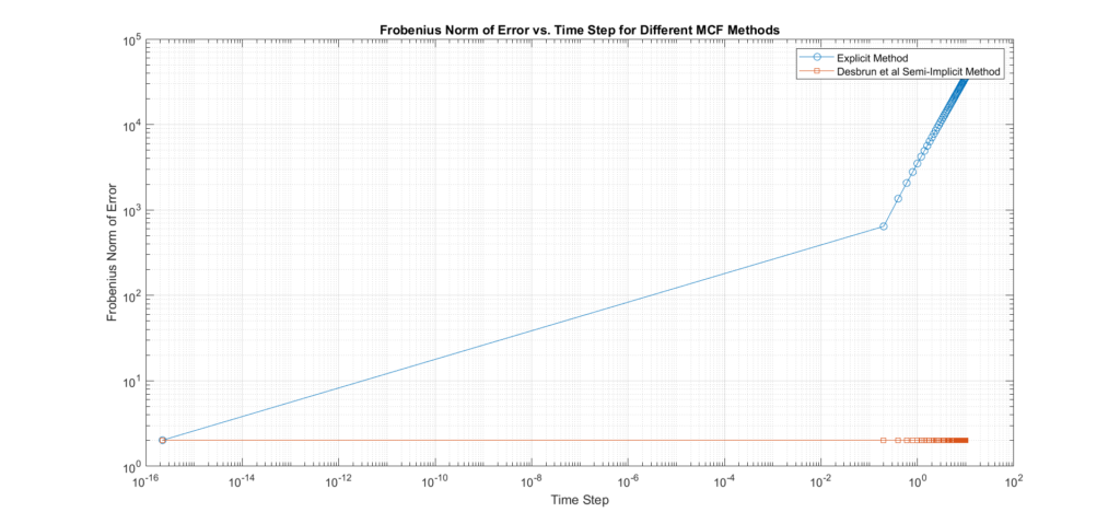
- Error vs. Time Steps: The error is plotted against the time step size on a log-log scale. The slope of this curve will indicate the convergence rate:
- Steeper Slope: Indicates faster convergence and higher accuracy.
- Flatter Slope: Suggests slower convergence and potential inaccuracies.
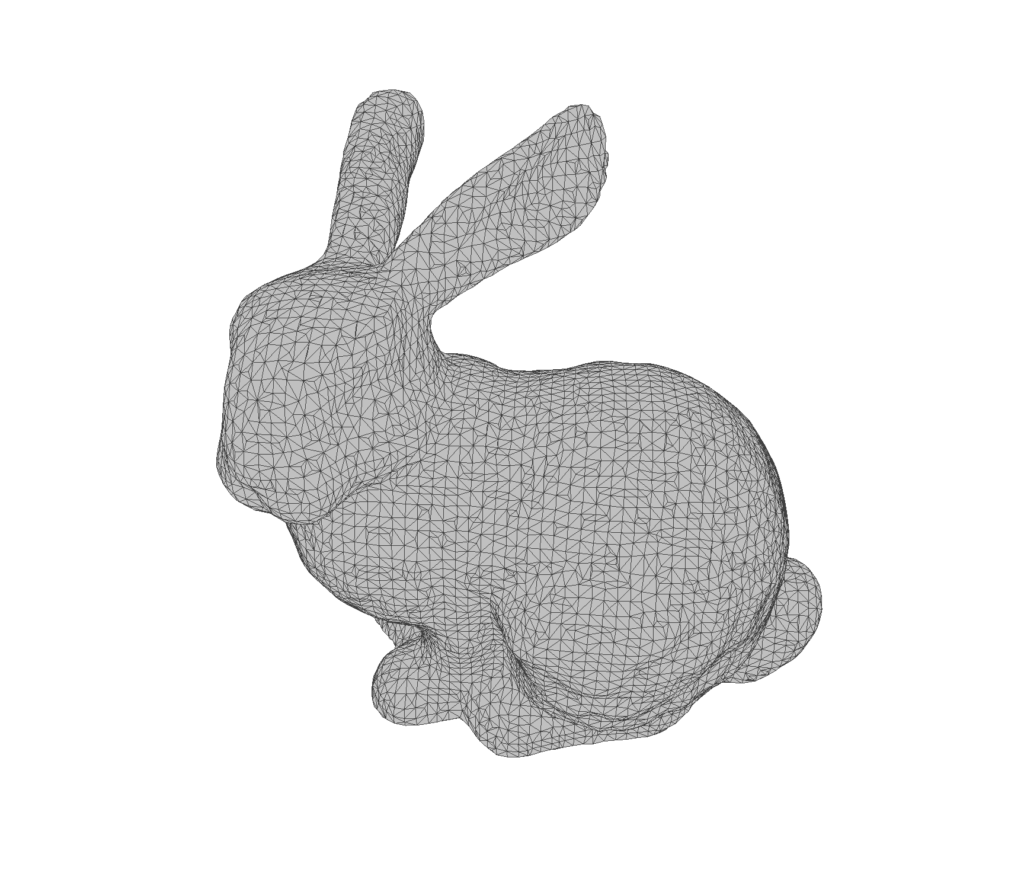
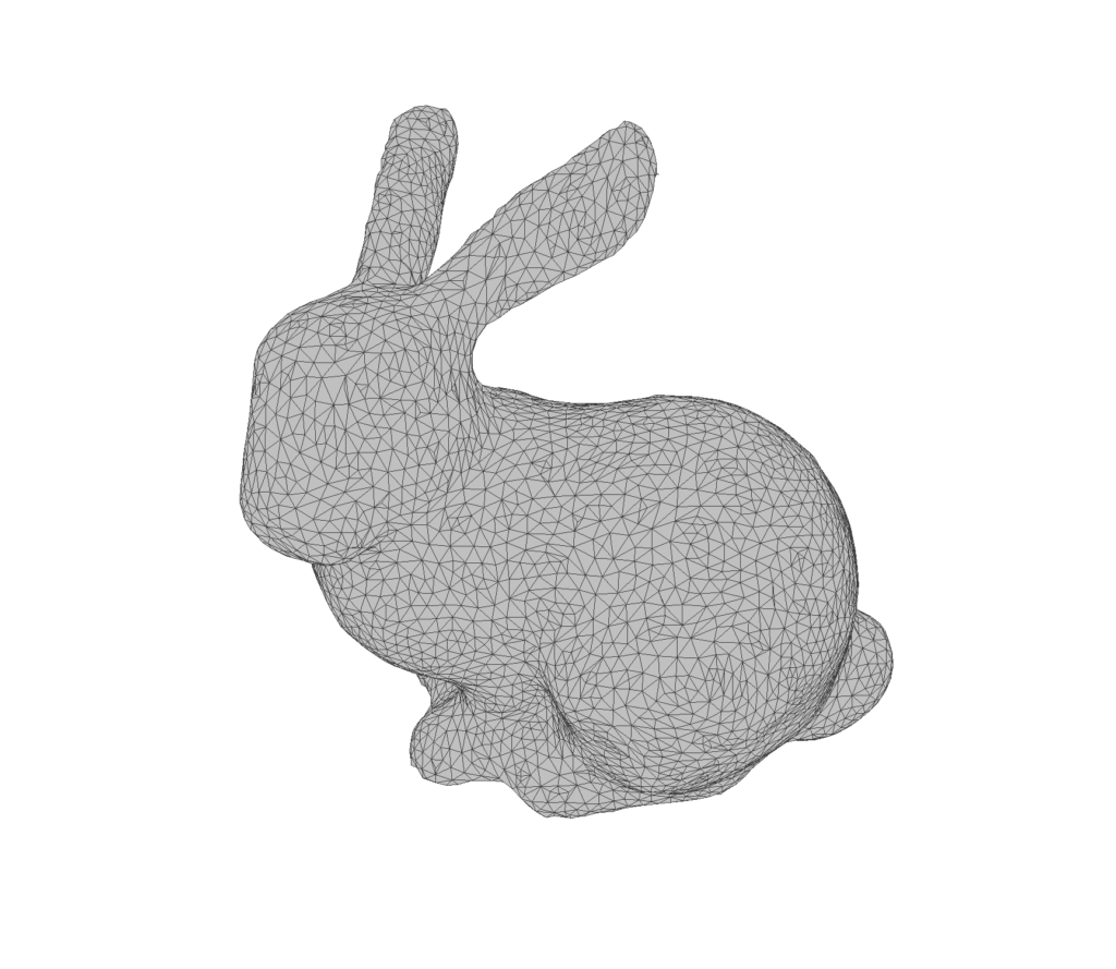
- Visual and Quantitative Evaluation: The final smoothed meshes are presented for visual comparison against the target mesh.
- Time Step Limitations: The maximum time step for which each method remains stable is identified.
- Error vs. Time Steps: The error is plotted against the time step size on a log-log scale. The slope of this curve will indicate the convergence rate:
Interpretation of Results:
- The accuracy plot shows that the Explicit method tends to produce much higher errors compared to the Desbrun’s especially at larger time steps, confirming that it requires small time steps to maintain stability. In addition, we can see that with Desbrun’s, the error remains constant across a wide range of varying time steps, this confirms that the method’s accuracy and stability are not affected by the choice of time step within the range tested, it also verifies its robustness, and tendency to reduce error propagation as time step sizes increase. In regards to the rate of convergence, the slope of the error curve vs time-steps in Euler’s explicit is \(m=1.29\), and Desbrun’s method rate of convergence is \(m=1\).
- In this experiment, we set the error threshold to 3. Turns out the maximum step size \(\Delta t\) where the error is below this threshold for Euler’s explicit is 2.2204e-16 while for Desbrun et al.’s is (the final in our range).
Inspiration: This experimental design was inspired by a task I did during my second SGI project on 2D Differentiable Representation of Curve Networks, under Mikhail Bessmeltsev. 🙂
The Case for Higher-Order Time Discretization
As demonstrated by both theory and practice, even robust methods like Desbrun et al.’s semi-implicit method for MCF face limitations with first-order time discretization. While this category of methods offers a compromise between explicit and fully implicit methods, first-order discretization still imposes constraints on accuracy in numerical simulations. These limitations stem from the truncation errors inherent in first-order approximations.
First-order methods approximate the time derivative using only vertex velocities (the first derivative of position with respect to time) and disregard higher-order terms, such as acceleration (the second derivative). This omission means they fail to account for how the geometry of the surface might be changing or accelerating locally since higher derivatives encode information about local curvatures. If we conceptualize the next iterate as\(X^{(k+1)}_i = \mu (X_i^{(k)}, I^{(k)})\) where \(I^{(k)}\) is an information vector, local geometric properties of the surface at the current iterate \(X_i^{(k)}\), it becomes clear that the more detailed information we incorporate into \(I^{(k)}\), the more accurate the next state \(X^{(k+1)}_i \) will be.
In other words, higher-order discretizations, such as second-order ones, lead to a significant reduction in truncation errors, better convergence, and a more accurate representation of the geometry over time for larger time steps which contributes to a more economical utilization of computational resources (e.g reduced number of iterations).
Deriving Higher-order Discretizations for MCF
In this section, we derive the second-order accurate, in time, vertex update rules for the explicit forward Euler and the semi-implicit due to Desbrun et al. Starting from the continuous form of the MCF equation, we use a Taylor expansion to approximate the position of a point on the surface up to the second-order term, and for Desbrun et al.’s, we make use of Neumann series in our derivation.
Recall that from the first section, the MCF in its continuous form, is described following equation:
\[\frac{\partial X(u,t)}{\partial t} = \Delta X(u,t)\]
where: \( X(u,t) \in \mathbb{R}^3 \) is the position of a point on the surface at parameter \( u \) and time \( t \), and \(\Delta\) is the Laplace Beltrami operator.
Now, we apply a Taylor expansion of \( X(u,t) \) around time \( t=t_k\):
\[ X(u, t_k + \Delta t) = X(u, t_k) + \Delta t \frac{\partial X(u,t)}{\partial t}| _{t=t_k}+ \frac{\Delta t^2}{2} \frac{\partial^2 X(u,t)}{\partial t^2}| _{t=t_k} + \mathcal{O}(\Delta t^3) \]
Substituting the MCF equation \( \frac{\partial X}{\partial t} = \Delta X \): \[ X(u, t_k + \Delta t) = X(u, t_k) + \Delta t \Delta X(u,t) | _{t=t_k}+ \frac{\Delta t^2}{2} \frac{\partial}{\partial t} \left( \Delta X(u,t) \right)| _{t=t_k} + \mathcal{O}(\Delta t^3) \]
Where, \[\frac{\partial^2 X(u,t)}{\partial t^2}\Bigg |_{t=t_k} = \frac{\partial}{\partial t} \left( \Delta X(u,t) \right) \Bigg |_{t=t_k}\] This follows from the definition of Laplace Beltrami operator and Schwarz’s Theorem (also known as Clairaut’s Theorem on Equality of Mixed Partials)
Now, \[ \frac{\partial}{\partial t} \left( \nabla X(u,t) \right) \Bigg |_{t=t_k} = \Delta \left( \frac{\partial X(u,t)}{\partial t} \right) \Bigg |_{t=t_k}= \Delta \left( \Delta X(u,t) \right) \Bigg |_{t=t_k} = \Delta^2 X(u,t) \Bigg |_{t=t_k} \]
By substituting this in Taylor’s expansion, we get the continuous second-order expansion for \( X(u,t)\) at \(t_k\):
\[ X(u, t_k + \Delta t) = X(u, t_k) + \Delta t \Delta X(u,t) \Bigg |_{t=t_k} + \frac{\Delta t^2}{2} \Delta^2 X(u,t) \Bigg |_{t=t_k} + \mathcal{O}(\Delta t^3) (*) \]
Now let \( X^{(k)}_i\), \( X^{(k+1)}_i \) denote the position vector of vertex \(i\) at times \( t_k \), and\( t_{k+1} \) respectively, and \( \Delta t = t_{k+1}-t_k\). Using the Taylor expansion in \((*)\), the second-order vertex update rule becomes:
\[ X^{(k+1)}_i\approx X^{(k)}_i + \Delta t \Delta X^{(k)}_i + \frac{\Delta t^2}{2} \Delta^2 X^{(k)}_i \]
Now the spatial discrete approximation we use in this article is \(\Delta \approx \mathbf{ML}^{-1}\). Now we can write the vertex update rule for Forward Euler as follows:
\[ X^{(k+1)}_i\approx X^{(k)}_i + \Delta t \mathbf{ML}^{-1} X^{(k)}_i + \frac{\Delta t^2}{2} (\mathbf{ML}^{-1})^2 X^{(k)}_i \]
After doing some algebra, we reach the following matrix form:
\[ X^{(k+1)} \approx [ I + \Delta t \mathbf{ML}^{-1} + \frac{\Delta t^2}{2} (\mathbf{ML}^{-1})^2] X^{(k)} \]
For the semi-implicit form due to Desbrun et al.’s, things are a bit tricky. It should be easy by now to derive the first-order vertex update presented earlier in (ref) using Taylor expansion which takes the matrix form:
\[X^{k+1}_i \approx (I- \Delta t\mathbf{M^{-1}L} X^{k} )^{-1} X^{k} \]
To derive the second order term for this scheme, we expand the inverse matrix \( \left(I – \Delta t \mathbf{M}^{-1} L X^{(k)} \right)^{-1} \) using a Neumann series, but for this to work, we have to ensure that \( \mathbf{M}^{-1}L X^{(k)}\) satisfies the condition for convergence, i.e., its spectral radius is strictly less than 1: \[ \rho (\Delta t \mathbf{M}^{-1}L X^{(k)} )<1 \]
This means \(\Delta t\) must be chosen small enough, or the structure of \(\mathbf{M}^{-1}L X^{(k)}\) must ensure that its eigenvalues are small.
Assuming this is true, the Neumann series expansion for \( \left(I – \Delta t \mathbf{M}^{-1}L X^{(k)} \right)^{-1} \) can be written as: \[ \left(I – \Delta t \mathbf{M}^{-1} L X^{(k)}\right)^{-1} = I + \Delta t \mathbf{M}^{-1} L X^{(k)}+ \Delta t^2 \left(\mathbf{M}^{-1} L X^{(k)}\right)^2 + \mathcal{O}(\Delta t^3)\]
Substituting this approximation into the semi-implicit update rule, we get:
\[ X^{k+1} \approx \left( I + \Delta t \mathbf{M}^{-1} L X^{(k)} + \Delta t^2 \left( \mathbf{M}^{-1} L X^{(k)} \right)^2 \right) X^{k} \qquad (***)\]
Discussion. The advantage of using Neumann series in deriving the second-order time discretization is that it allows us to approximate \( \left(I – \Delta t \mathbf{M}^{-1} L X^{(k)} \right)^{-1} \) without having to directly compute the matrix inverse, which can be computationally expensive for large meshes. Instead, the expansion provides a series of manageable terms so with that we can economically exploit the accuracy benefits attained from adding the higher-order terms. With that said, the major disadvantage here is that if \(\Delta t\) becomes too large, the Neumann series may fail to converge or lead to unstable behavior, limiting a bit its effectiveness for semi-implicit schemes over larger intervals. However, it would be not correct to say that it is impossible to circumvent the stability issue. We talk about this in a subsequent article.
An Alternative Discretization based on (Huisken’s, 1984) MCF Evolution Equations
Earlier in the article, we mentioned the landmark result of the influence of MCF on strictly convex smooth hypersurface in Euclidean spaces due to (Huisken, 1984). To establish this result, Huisken derived several key equations that rigorously describe how various geometric quantities change over time as general surfaces evolve under MCF.
- \( \frac{\partial n}{\partial t}=\nabla H \)
- \( \frac{\partial H}{\partial t}=\Delta H+|A|^2 H =\Delta H + (H^2-2K)H. \) where \(A\) is the second fundamental form, and \(K\) is the Gaussian curvature.
These are called the surface evolution equations, The first equation describes how the unit normal vector \(n\) evolves over time, linking its rate of change to the gradient of the mean curvature \(H\). The second equation tracks the evolution of \(H\) itself as the surface changes.
From these, we can derive the following equation for the second derivative of the surface position \(X\) with respect to time:
\[\frac{\partial^2 X}{\partial t^2} = \frac{\partial}{\partial t}(H\mathbf{n}) = \frac{\partial H}{\partial t}\mathbf{n} + H\frac{\partial \mathbf{n}}{\partial t}= (\Delta H +(H^2-2K)H)\mathbf{n}+H\nabla H\]
This expression consists of geometric quantities that can be approximated on a mesh—though they tend to be noisy. We can also write the equation in an alternative form:
\[\frac{\partial^2 X}{\partial t^2}=(\Delta H)\mathbf{n} + (H^2-2K)\Delta x + H\nabla H\]
Why is this important here? Since we are discussing higher-order discretizations of MCF, we are interested in discovering new equivalent (and hopefully economical) ways to describe the temporal derivatives in question. (Huisken, 1984) provides some, and thus a natural question arises: can we discretize the components, \(\mathbf{n}, H, \Delta H, \nabla H, K\) of \( \frac{\partial^2 X}{\partial t^2}\) and \(\frac{\partial X}{\partial t}\) to derive a second-order discretization for MCF using Taylor series? The answer is yes.
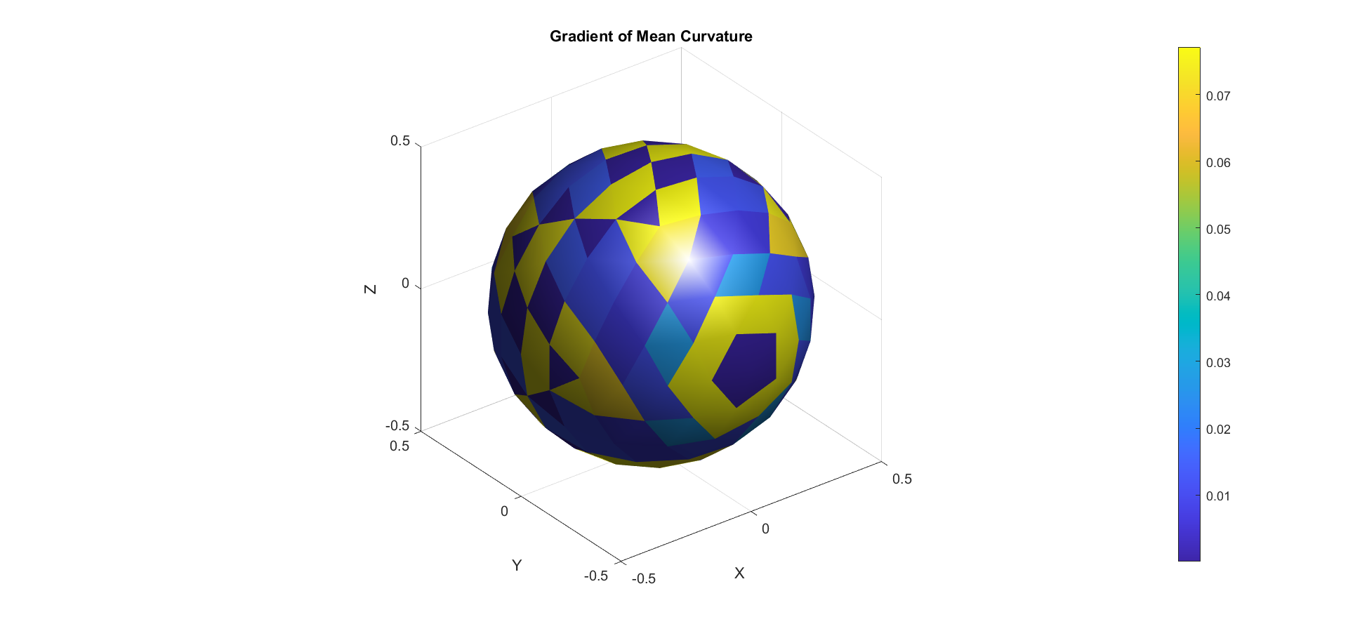
For example, the Gaussian curvature \(K\) can be discretized using the angle deficit method. The normal vector \(\mathbf{n}\) at a vertex can be estimated as the area-weighted average of the normals of the adjacent triangles. The mean curvature \(H\) as \(\mathbf{M^{-1}L}\) applied to the verticies of the mesh. The gradient \(\nabla H\) can be approximated using finite differences or based on the stiffness matrix \(mathbf{L}\) and adjacent vertex data, while \(\Delta H\) can be discretized using \(\mathbf{L}\) applied to the discrete mean curvature \(H\).
Using these discretized quantities, we arrive at the following vertex update formula: \[ X_i^{(k+1)} \approx X_i^{(k)}+\Delta t H_i \mathbf{n}_i + \frac{\Delta t^2}{2} ( (\mathbf{L} H_i) \mathbf{n}_i + (H_i^2-2K_i)\Delta X_i^{(k)} + H_i\nabla H_i)) \] However, as mentioned this discretization approach is often not preferred due to the significant noise in the quantities \(\mathbf{n}, H, \Delta H, \nabla H\), and \(K\) on meshes.
Visualizing \(n, H, \Delta H, \nabla H,\) and \(K\) on a Mesh
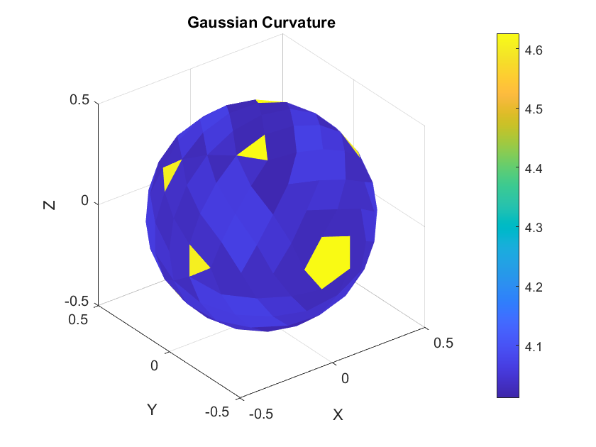
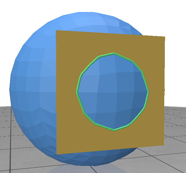
Gaussian curvature
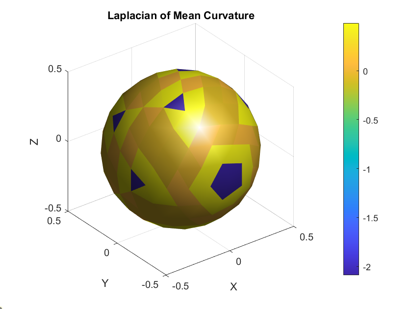
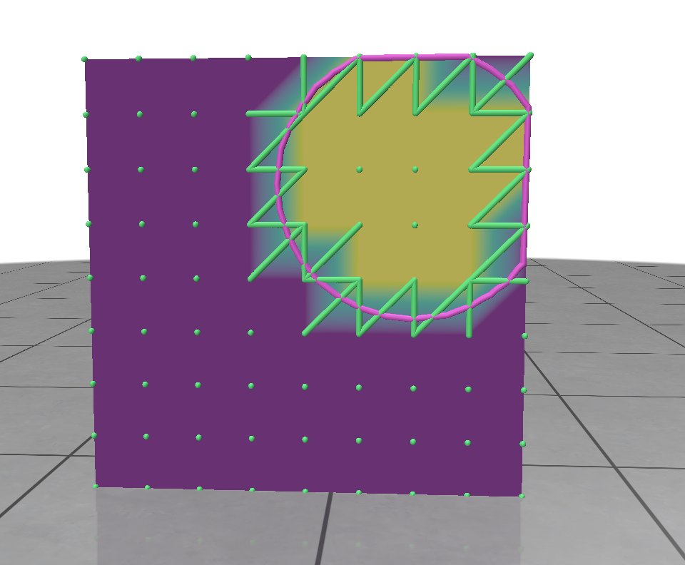
Laplcian of mean curvature
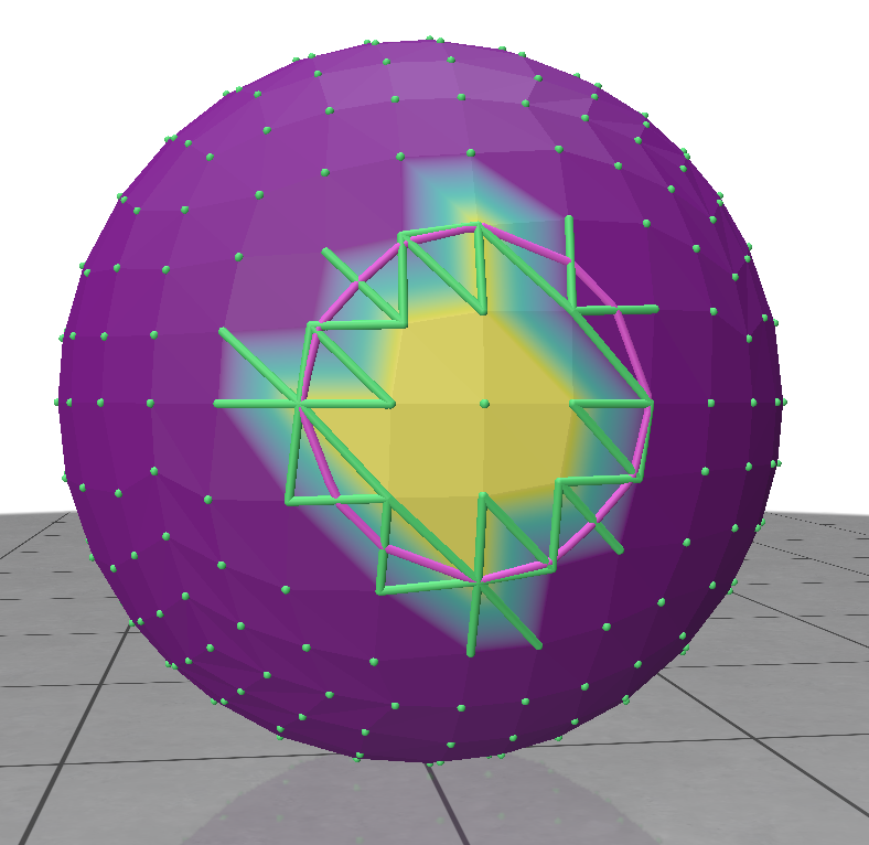
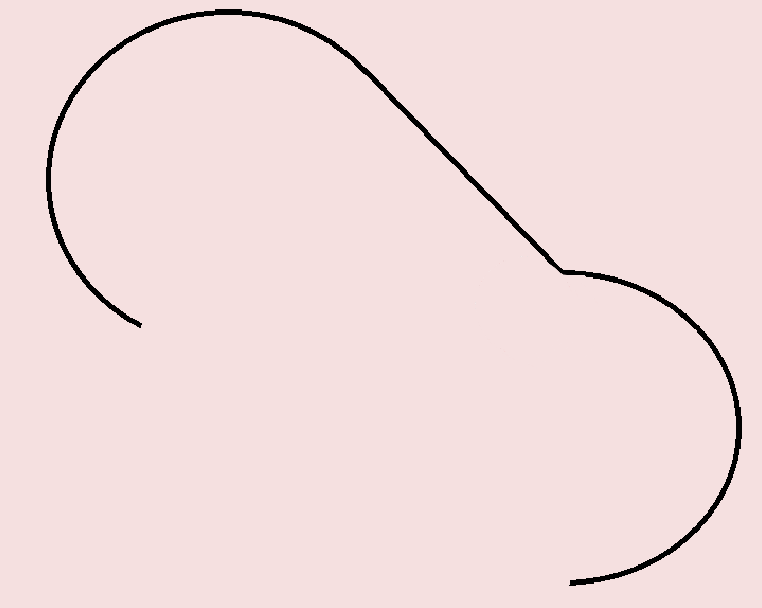
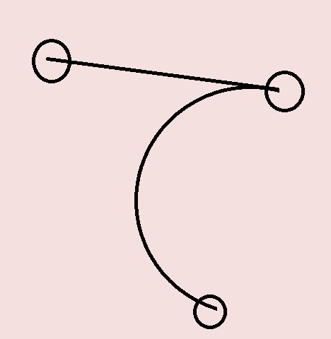
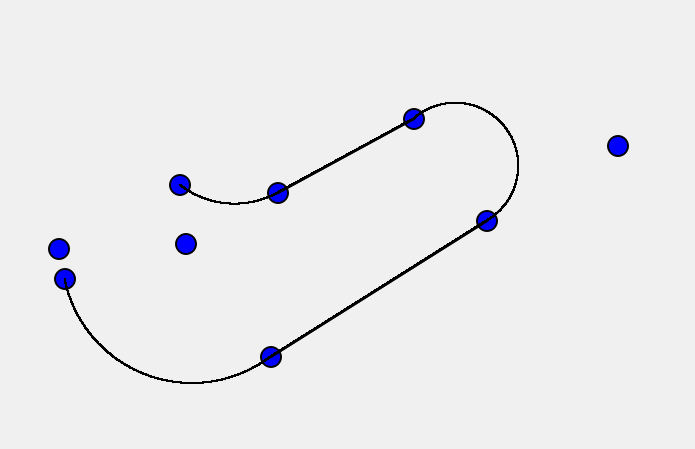
The next experiment aims to visualize higher-order effects in MCF by plotting small arcs at each mesh vertex. These arcs are defined as
\(f(h) = X_i + (Hn) \big |_{X=X_i} \cdot h + \frac{1}{2} (\frac{\partial}{\partial t}(Hn))\big |_{X=X_i}= \frac{\partial H}{\partial t}n \big |_{X=X_i}+ H\frac{\partial n}{\partial t}\big |_{X=X_i}= (\Delta H +(H^2-2K)H)n \big |_{X=X_i}+H\nabla H) \big |_{X=X_i} \cdot h^2 \)
where \(\frac{\partial X}{\partial t}\) is the mean curvature normal and \(\frac{\partial^2X}{\partial t^2}\) is a second-order term from Huisken’s calculations.
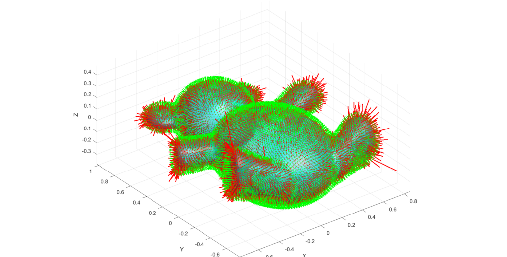
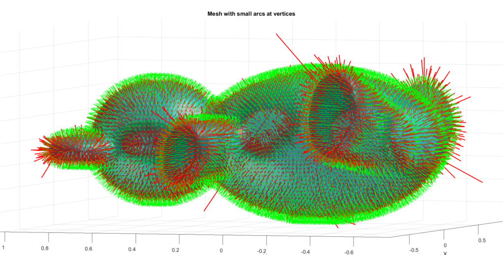
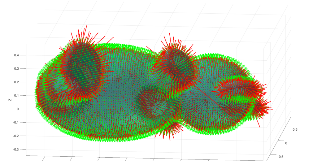
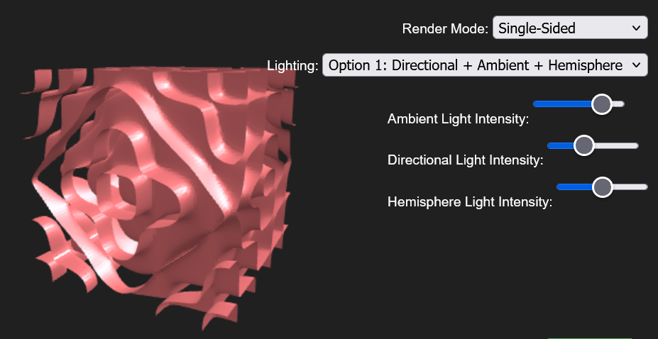
The first-order term moves the surface in the direction of the normal, scaled by the mean curvature. This means regions with higher curvature see greater movement compared to flatter regions. The second-order term refines this by adding curvature-dependent corrections. It can enhance or counteract the displacement done via the first-order term, affecting the arc’s bending and potentially leading to different geometric changes. In addition, the second-order term can indeed add accuracy to the displacement, providing a more precise description of surface evolution. However, higher-order terms are also more sensitive to mesh noise and discretization errors, which can introduce potential instabilities or oscillations, particularly in regions with poor mesh quality and such instabilities can be amplified in regions with high curvature, where numerical errors from the second-order term might dominate. In our case, these instabilities are reflected in exaggerated displacements, resulting in disproportionately large polylines at certain vertices. With more trivial meshes, this instability problem will not be as amplified as it is the case with complex meshes.
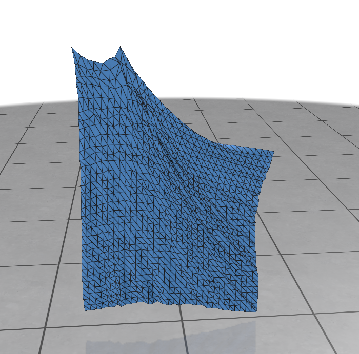
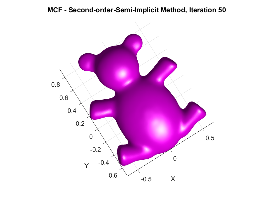
Implementation of Second-Order Semi-implicit (Desbrun et al.’s, 1999):
The following are the output results of our second-order Desbrun et al’s semi-implicit method (\(***\)).
Yay or Nay: Circular Arc-Based Discretizations for Curvature-Driven Flows
In the Taylor expansion used to derive the vertex-update rule for MCF, the position \(X(u,t)\) of each vertex is typically approximated by a quadratic polynomial in time:
\[ X(u, t_k + \Delta t) = X(u, t_k) + \Delta t \frac{\partial X(u,t)}{\partial t}| _{t=t_k}+ \frac{\Delta t^2}{2} \frac{\partial^2 X(u,t)}{\partial t^2}| _{t=t_k} + \mathcal{O}(\Delta t^3) \]
where \( \frac{\partial X}{\partial t} = \Delta X \), the Laplacian of the position, is the driving term in MCF, and \( \frac{\partial^2 X}{\partial t^2} \) is obtained from differentiating this expression again. While this quadratic approximation is computationally straightforward and effective for small time steps, it does not inherently capture the geometric structure of the flow.
For curvature-driven flows, such as the evolution of a sphere under MCF, where the curvature \( H \) is constant at each point, circular arcs may provide a more natural approximation. Circular arcs reflect the constant curvature evolution by following a trajectory where the velocity of each vertex aligns with the normal direction, and the path of the vertex forms part of a circle. This would involve approximating the update as:
\[X(u, t_k + \Delta t) \approx X(u, t_k) + r(\cos(\theta) – 1) \mathbf{n},\]
where \( r \) is the radius of curvature and \( \theta \) is the angle swept by the vertex in time \( \Delta t \), with \( \mathbf{n} \) being the surface normal. While circular arcs introduce more computational complexity, they better approximate the geometric behavior of curvature-dominated flows and may lead to improved accuracy and stability in such cases.
Key Takeaway:
- MCF is important in GP!
- Lots of discretization approaches for the Laplacian exist, none of them could keep every natural property of its ideal continuous form. You choose what is suitable for your problem, and application.
- Coming up with new equivalent formulations for MC \(H\), and the rate of change of the position vector-valued function \(X\) of points on the surface would open more doors for finding new economical discretizations
Future work: Will venture more into the math of MCF, focusing specifically on points 2 and 3 from the Key Takeaways. Additionally, I explore some tangentials in regards to higher-order integrators for MCF, and other geometric flows.
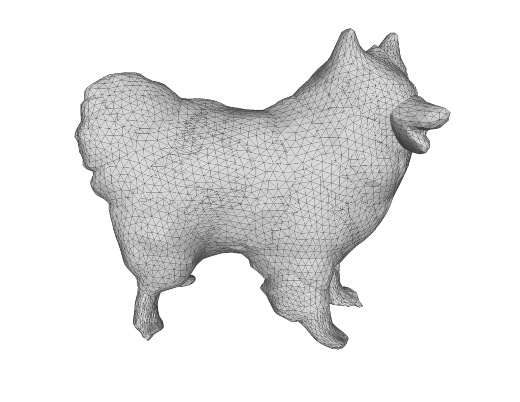
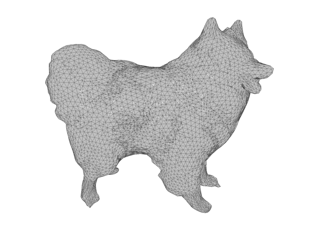
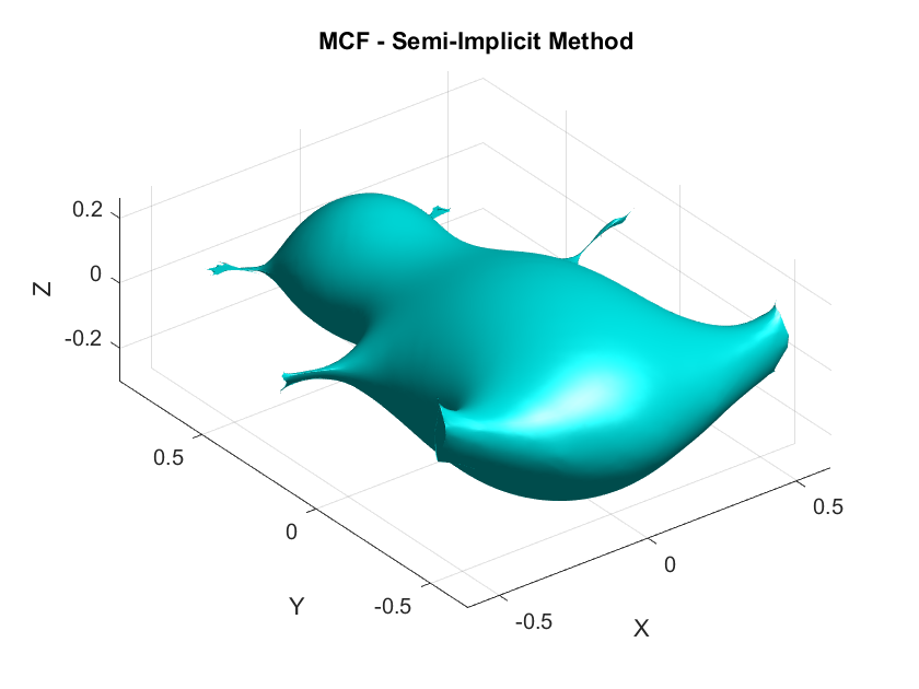
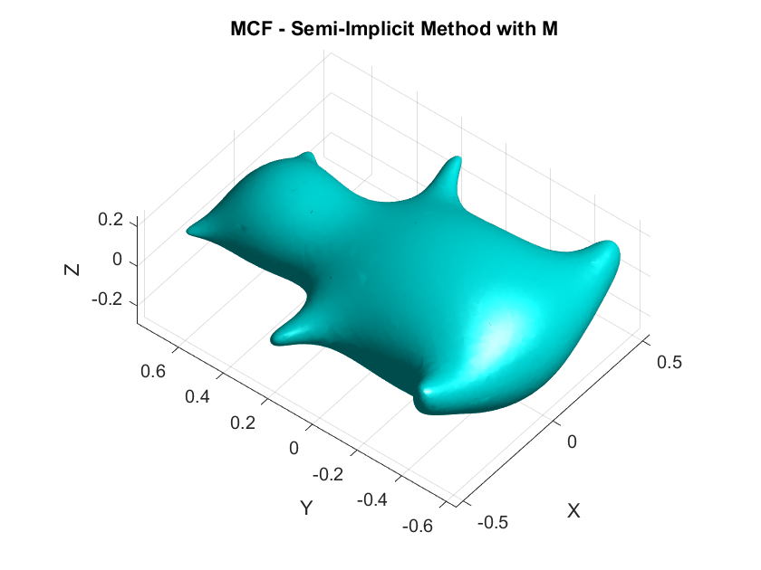
A Humorous Fail:
On the second day while coding the first-order discretizations, I forgot to include the mass matrix \(\mathbf{M}\) which resulted in a smoothed horribly deformed bear. This demonstrates the critical role of \(\mathbf{M}\) in ensuring that the discretization respects the surface’s geometry by appropriately distributing weight across the vertices according to the areas of the surrounding triangles.
- When the basis functions used are piecewise linear and the mesh structure is uniform ↩︎
Bibiliography:
- Justin Solomon (Director). (2013, May 8). Lecture 12: Finite Elements and the Laplacian [Video recording]. https://www.youtube.com/watch?v=7_xDIg-pOC4
- Huisken, G. (1984). Flow by mean curvature of convex surfaces into spheres. Journal of Differential Geometry, 20(1), 237-266.
- Desbrun, M., Meyer, M., Schröder, P., & Barr, A. H. (1999, July). Implicit fairing of irregular meshes using diffusion and curvature flow. In Proceedings of the 26th annual conference on Computer graphics and interactive techniques (pp. 317-324).
- Patanè, G. (2017). An introduction to Laplacian spectral distances and kernels: Theory, computation, and applications. In ACM SIGGRAPH 2017 Courses (pp. 1-54).
- Hughes, T. J. R. (2000). The finite element method: Linear static and dynamic finite element analysis. Dover Publications.
- Evans, L. C. (2010). Partial differential equations. American Mathematical Society.