This is the 2nd part of the two-part post series, prepared by Krishna and I. Krishna presented an overview of SLAM systems in a very intuitive and engaging way. In this part, I explore the future of SLAM systems in endoscopy and how our team plans to shape it.
Collaborators: Krishna Chebolu
Introduction
What about the future of SLAM endoscopy systems? To get an insight on where research is heading, we must first discuss the challenges posed by the task to localise an agent and map such a difficult environment, as well as the weaknesses of current systems.
On one hand, the environment of the inside of the human body, coupled with data/device heterogeneity and image quality issues, significantly hinder the performance of endoscopy SLAM systems [1], [2] due to:
1) Texture scarceness, scale ambiguity
2) Illumination variation
3) Bodies (foreign or not), fluids and their movement (e.g., mucus, mucosal movement)
4) Deformable tissues and occlusions
5) Scope-related issues (e.g., imagery quality variability)
6) Underlining scene dynamics (e.g., imminent corruption of frames with severe artefacts, large organ motion and surface drifts)
7) Data heterogeneity (e.g., population diversity, rare or inconspicuous disease cases, variability in disease appearances from one organ to the other, endoscope variability)
8) Difference in device manufacturers
9) Input of experts being required for their reliable development
10) The organ preparation process
11) Additional imaging quality issues (e.g. free/non-uniform hand motions and organ movements, different image modalities)
12) Real time performance (speed and accuracy trade-off)
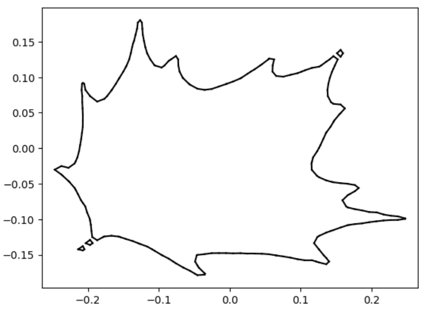
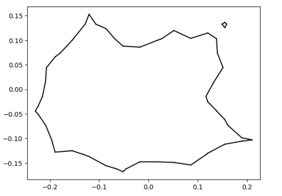
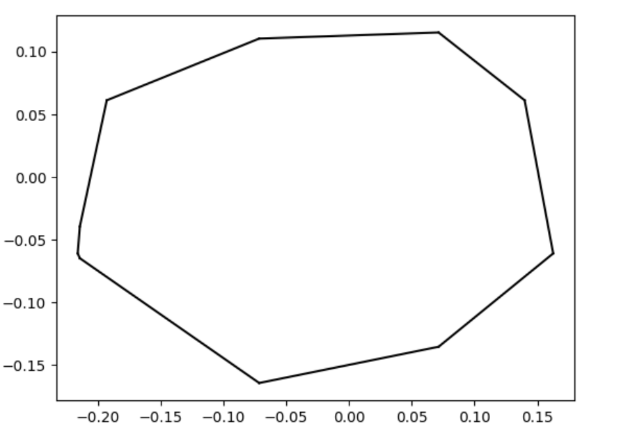
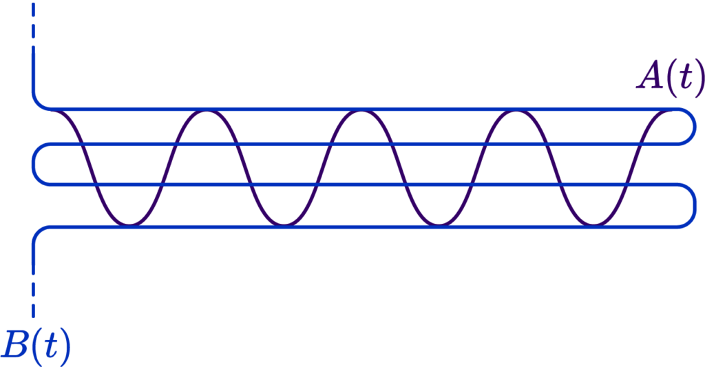
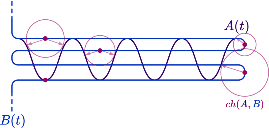
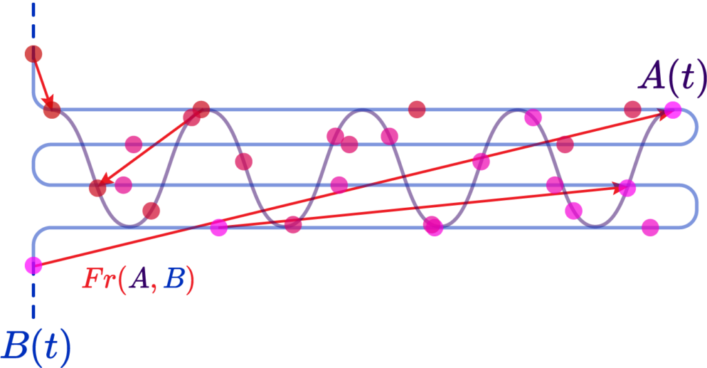
Current research of endoscopic SLAM systems mainly focuses on the first 3 of the aforementioned challenges; the state-of-the-art pipelines focus on understanding depth despite the lack of texture, as well as handling lighting changes and foreign bodies like mucus that can be reflective or move and, thus, skew the mapping reconstruction.

Images 1, 2, 3: The images above showcase the three main problems that skew the tissue structure understanding and hinder the performance of mapping of SLAM systems in endoscopy: (1) foreign bodies that are reflective (2) lighting variations and (3) lack of texture. Image credits: [3], [3], [4].
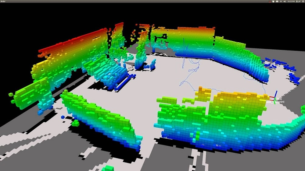
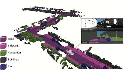
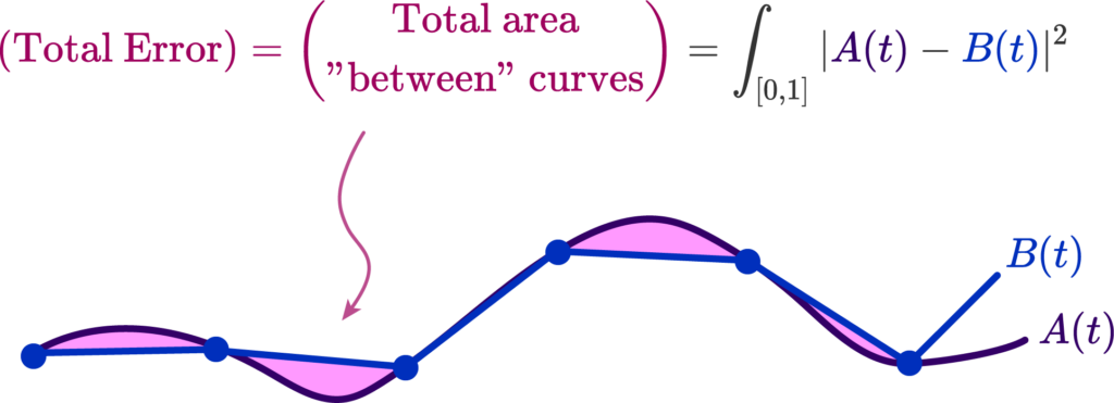
On the other hand, we must pinpoint where the weaknesses of such systems lie. The three main modules of AI endoscopy systems, that operate on image data, are Simultaneous Localization and Mapping (SLAM), Depth Estimation (DE) and Visual Odometry (VO); with the last two being submodules of the broader SLAM systems. SLAM is a computational method that enables a device to map its environment while simultaneously determining its own position within that map, which is often achieved via VO; a technique that estimates the camera’s position and trajectory by examining changes across a series of images. Depth estimation is the process of determining the distance between a camera and the objects in its view by analyzing visual information from one or more images, which is crucial for SLAM to accurately map the environment in three dimensions and understand its surroundings more effectively. Attempting to use general purpose SLAM systems on endoscopy data clearly shows that DE and map reconstruction are underperforming, while localisation/VO is sufficiently captured. This conclusion was reached based on initial experiments; however, further investigations are warranted.
Though the challenges and system weaknesses that current research aims to address are critical aspects of the models’ usability and performance, there is still a wide gap between the curated settings under which these models perform and real-world clinical settings. Clinical applications are still uncommon, due to the lack of holistic and representative datasets, in conjuction with limited participation of clinical experts. This leads to models that lack generalisability; widely used supervised techniques are data voracious and require many human annotations, which, apart from scarce, are often imperfect or overfitted to predominant samples in cohorts. Novel deep learning methods should be steered towards training on diverse endoscopic datasets, the introduction of explainability of results and the interpretability of models, which are required to accelerate this field. Finally, suitable evaluation metrics (i.e. generalisability assessments and robustness tests) should be defined to determine the strength of developed methods in regards to clinical translation.
For a future of advanced and applicable AI endoscopy systems, the directions are clear, as discussed in [1]:
1) Endoscopy-specific solutions must be developed, rather than just applying pipelines from the computer vision field
2) Robustness and generalisation evaluation metrics of the developed solutions must be defined to set the standard to assess and compare model performance
3) Practicability, compactness and real time effectiveness should also be quantified
4) More challenging problems should be explored (subtle lesions instead of apparent lesions)
5) The developed models should be able to adapt to datasets produced in different clinics, using different endoscopes, in the context of varying manifestations of diseases
6) Multi-modal and multi-scale integration of data should be incorporated in these systems
7) Clinical validation is necessary to steadily integrate these systems in the clinical process
Method
But how do we envision the future of SLAM endoscopy systems?
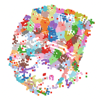
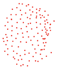
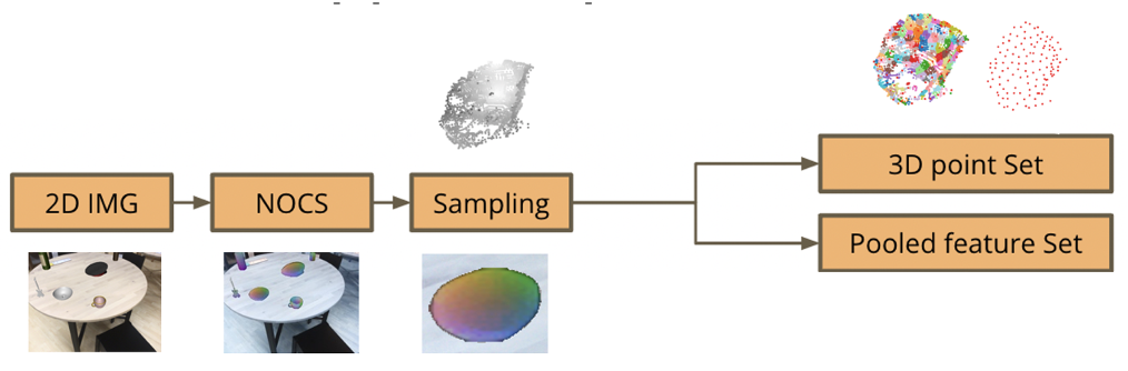
Our team aims to address directly the issues of texture scarceness, illumination variation and handling of foreign bodies, while indirectly combating some of the rest of the challenges. Building upon state-of-the-art SLAM systems, which already handle localisation/VO sufficiently, we aim to further enhance their mapping process, by integrating a state-of-the-art endoscopy monocular depth estimation pipeline [3] and by developing a module to understand lighting variations in the context of endoscopic image analysis. The aforementioned module will have a corrective nature, automatically adjusting the lighting in the captured images to ensure that the visuals are clear and consistent. Potentially, it could also enhance the image quality by adjusting brightness, contrast, and other image parameters in real-time, standardizing the images of different frames of the endoscopy video. As the module’s task is to improve the visibility and consistency of the image features, it would consequentially also support the depth estimation process, by providing clearer cues and contrast for accurate depth calculations by the endoscopy monocular depth estimation pipeline. Thus, the module would ensure a more consistent and refined input to the SLAM model, rather than raw endoscopy data, which suffer from inconsistencies and heterogeneities, never seen before by the model. With the aforementioned integrations we aim to develop a specialised SLAM endoscopy system and test it in the context of clinical colonoscopy [5]. Ideally, the plan is to first train and test our pipeline on a curated dataset to test its performance under controlled settings and then it would be of great interest to adjust each part of the pipeline to make it perform on real-world clinical data or across multiple datasets. This will provide us with the opportunity to see where a state-of-the-art SLAM endoscopy system stands in the context of real-world applicability and help quantify and address the issues explored in the previous section.
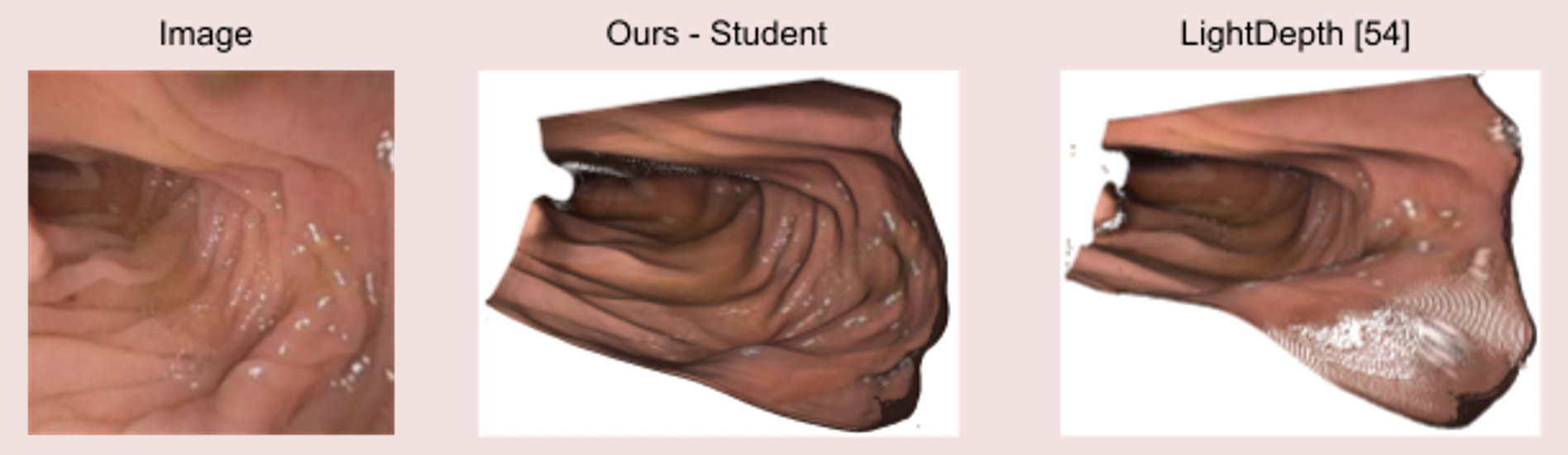
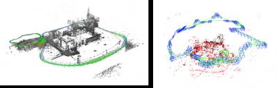
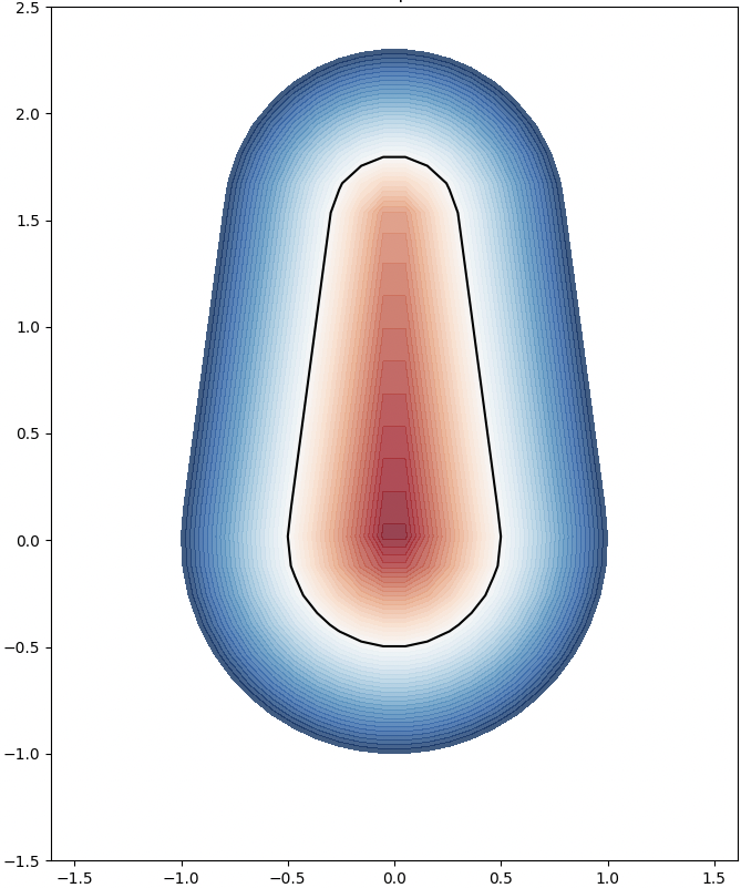
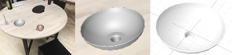
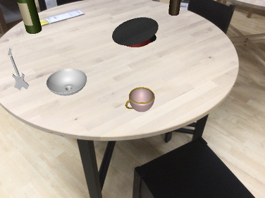
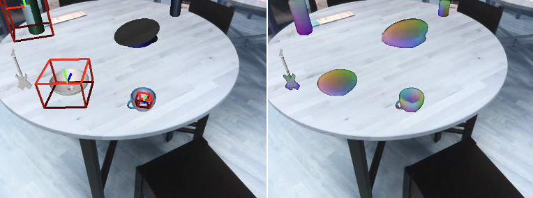
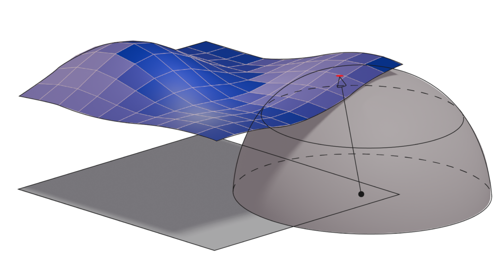
Image 4: State-of-the-art clinical mesh reconstruction using the endoscopy monocular depth estimation pipeline [5].

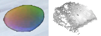
Image 5: The endoscopy monocular depth estimation pipeline also extracts state-of-the-art depth estimation in endoscopy videos.
Colonoscopy Data
The type of endoscopy procedure we choose to develop our pipeline for is colonoscopy; a medical procedure that uses a flexible fibre-optic instrument equipped with a camera and light (a colonoscope) to examine the interior of the colon and rectum. More specifically, we select to work with the Colonoscopy 3D Video Dataset (C3VD) [5]. The significance of this dataset study is the fact that it provides high quality ground truth data, obtained using a high-definition clinical colonoscope and high-fidelity colon models, creating a benchmark for computer vision pipelines. The study introduced a novel multimodal 2D-3D registration technique to register optical video sequences with ground truth rendered views of a known 3D model.
Video 1: C3VD dataset: Data from the colonoscopy camera (left) and depth estimation (right) extracted by a Generative Adversarial Network (GAN). Video credits: [5]
Conclusion
SLAM systems are the state-of-the-art for localisation and mapping and endoscopy is the gold standard procedure for many hollow organs. Combining the two, we get a powerful medical tool that can not only improve patient care, but also be life-defining in some cases. Its use cases can be prognostic, diagnostic, monitoring and even therapeutic, ranging from, but not limited to: disease surveillance, inflammation monitoring, early cancer detection, tumour characterisation, resection procedures, minimally invasive treatment interventions and therapeutic response monitoring. With the development of SLAM endoscopy systems, the endoscopy surgeon has acquired a visual overview of various environments inside the human body, that would otherwise be impossible. Endoscopy being highly operator-dependent with grim clinical outcomes in some disease cases, makes reliable and accurate automated system guidance imperative. Thus, in recent years, there has been a significant increase in the publication of endoscopic imaging-based methods within the fields of computer-aided detection (CADe), computer-aided diagnosis (CADx) and computer-assisted surgery (CAS). In the future, most designed methods must be more generalisable to unseen noisy data, patient population variability and variable disease appearances, giving an answer to the multi-faceted challenges that the latest models fail to address, under actual clinical settings.
This post concludes part 11 of What it Takes to Get a SLAM Dunk.

Image 6: Michael Jordan (considered by me and many as the G.O.A.T.) performing his most famous dunk. Image credits: ScienceABC
References
[1] Ali, S. Where do we stand in AI for endoscopic image analysis? Deciphering gaps and future directions. npj Digit. Med. 5, 184 (2022). https://doi.org/10.1038/s41746-022-00733-3
[2] Ali, S., Zhou, F., Braden, B. et al. An objective comparison of detection and segmentation algorithms for artefacts in clinical endoscopy. Sci Rep 10, 2748 (2020). https://doi.org/10.1038/s41598-020-59413-5
[3] Paruchuri, A., Ehrenstein, S., Wang, S., Fried, I., Pizer, S. M., Niethammer, M., & Sengupta, R. Leveraging near-field lighting for monocular depth estimation from endoscopy videos. In Proceedings of the European Conference on Computer Vision (ECCV), (2024). https://doi.org/10.48550/arXiv.2403.17915
[4] https://commons.wikimedia.org/wiki/File:Stomach_endoscopy_1.jpg
[5] Bobrow, T. L., Golhar, M., Vijayan, R., Akshintala, V. S., Garcia, J. R., & Durr, N. J. Colonoscopy 3D video dataset with paired depth from 2D-3D registration. Medical Image Analysis, 102956 (2023). https://doi.org/10.48550/arXiv.2206.08903