RXMesh is a framework for processing triangle mesh on the GPU. It allows developers to easily use the GPU’s massive parallelism to perform common geometry processing tasks on triangle mesh. For a preliminary introduction to RXMesh, check out this tutorial blog here.
Our task was to use RXMesh to implement some classic algorithms in geometry processing. This blog details one of the algorithms we implemented: Spectral Conformal Parameterization (SCP).
This blog will discuss the algorithm in terms of its basic concepts, the steps of the algorithm, the implementation using RXMesh, and our results.
Our entire implementation of SCP application in RXMesh can be found here.
Spectral Conformal Parameterization
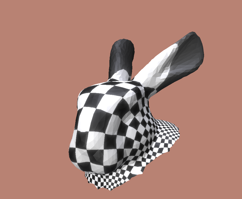
Parameterization refers to the mapping of a triangle surface mesh in \(R^{3}\) space to a planar \(R^{2}\) space. This mapping can then be subsequently used in different application such as texture mapping, where we map the values from some other \(R^{2}\) space (e.g., image) to the surface of the mesh. In this case, we map color values to the mesh surface.
Often when we perform mesh parameterization, there is a possibility to change some properties of the geometric elements of the mesh, such as the size, shape, or angle between edges. It is desired to preserve these properties since we usually want to create a direct mapping of our intended values (e.g., texture color) to be in the “correct” positions on the mesh. What is correct is usually up to artistic opinion, and thus a mapping that preserves these properties is desirable. A mapping that conserves angles (and thus shape) is called a conformal mapping.
Mullen et al. (2008) provides a method to perform conformal parameterization of an open surface mesh by modelling the problem as a generalized Eigenvalue problem. Using an initial guess, we can perform multiple iterations of a general eigen vector solving method (i.e., the power method [2] ) to determine the largest eigen vector. This eigen vector, in our case, is the parameterized coordinates of the given mesh, giving us our desired output.
To find the eigenvector \(u\), we can the power method since the problem is in the form \(B y_{k+1} = A x_{k}\). This can be done in the following way:
Where \(u\) is the parameterized coordinates. \(T1\) and \(T2\) are temporary variables to store certain scalar or vector values. Other variables are explained by Mullen et al. (2008). This loop can be implemented like this using RXMesh:
\(T1\) is a vector whose values are per-vertex, which is why we perform a per vertex computation. \(T2\) is a scalar in which we store the value of the dot product dot(eb,uv).
Since our system matrix \(L_{c}\) has dimensions 2V x 2V, we use complex representations of value entries in the vectors and matrices we use. So, for example, our \(L_{c}\) matrix now has dimensions V x V where each entry is a complex number (with a real and complex part).
This means subsequent computations must use CUDA functions that operate on complex numbers (e.g., cuCsubf which subtracts complex numbers).
All initial pre-computations only allocate to the real part of the entry, except for the calculation of the area term \(A\) where we calculate \(L_{c}=L_{D}-A\) . For the area term, we assign values to the complex part of the area term. \(L_{D}\) represents the standard Laplace-Beltrami operator, which we calculate using the cotangent edge weights and assign to the real part.
After we obtain the eigenvector \(u\) in complex form, we can convert it to a standard V x 2 matrix form and use that for further processing (such as rendering).
Results
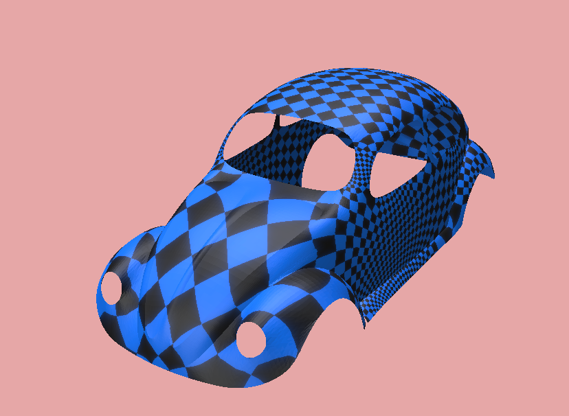
Using the SCP implementation, we can now apply texturing to our open meshes as shown in the examples below.
[2] Kozłowski, W. (1992). The power method for the generalized eigenvalue problem. Roczniki Polskiego Towarzystwa Matematycznego. Seria 3, Matematyka Stosowana/Matematyka Stosowana/Mathematica Applicanda, 21(35). https://doi.org/10.14708/ma.v21i35.1790
This blog was written by Sachin Kishan and Diany Pressato during the SGI 2024 Fellowship as one of the outcomes of a two-week project under the mentorship of Ahmed Mahmoud and the support of Supriya Gadi Patil as a teaching assistant.
RXMesh is a framework for processing triangle mesh on the GPU. It allows developers to easily use the GPU’s massive parallelism to perform common geometry processing tasks. For a preliminary introduction to RXMesh, check out this tutorial blog here.
Our task was to use RXMesh to implement some classic algorithms in geometry processing. This blog details one of the algorithms we implemented: As-Rigid-As-Possible(ARAP) Surface Modeling [1].
This blog will discuss the algorithm in terms of its basic concepts, the steps of the algorithm, the implementation using RXMesh, and the final results.
Our entire implementation of ARAP deformation in RXMesh can be found here.
As-Rigid-As-Possible Surface Modeling
Sorkine and Alexa (2007) formulated a method where we can retain the shape of an object as much as possible despite deforming one (or a set of) its vertices. This retention of shape is achieved by ensuring that subsequent transformations to the mesh after deforming its vertices are rigid. This property of rigidity means that a mesh can only undergo rigid transformations such as translation or rotation, but not stretching or shearing (since these are not rigid transformations).
The algorithm’s focus is to minimize the energy which measures the extent of deformation (dubbed rigidity energy). This energy is minimized when given a specific set of positions or a specific set of rotations. Notice that we can not minimize both at once—since we need the minimized rotational transformation for minimizing the energy from deformed positions. Thus, we instead solve both alternatively, i.e., solve for deformed positions assuming rotation is fixed, then solve for rotation assuming the position is fixed.
Using a Laplacian, we can form a sparse system of linear equations which we can then solve to obtain a new set of positions for the mesh. The algorithm works as follows for a single iteration
Identify the rotation matrix for the given deformed positions which minimizes deformation energy.
Solve for the new positions to minimize the energy, given a set of linear equations.
In this case, the set of linear equations to solve is in the form :
\(Lx=b\)
Where \(L\) is the Laplace-Beltrami operator, which can be formed by finding the cotangent edge weights of the mesh, \(x\) represents the set of new vertex positions we solve for, and \(b\) represents the right-hand side of Equation 8 from Sorkine and Alexa (2007). The derivation is detailed further in the original paper.
To further minimize the energy, we can perform multiple iterations of the same steps, using updated vertex positions and consequent rotations per iteration.
Implementation
The following code snippets show how the algorithm is implemented in RXMesh.
We first deform the input mesh and set constraints on each vertex depending on whether it is fixed, deformed, or free to move. This will be taken into account when calculating the system matrix \(L\).
 // set constraints
    const vec3<float> sphere_center(0.1818329, -0.99023, 0.325066);
    rx.for_each_vertex(DEVICE, [=] __device__(const VertexHandle& vh) {
        const vec3<float> p(deformed_vertex_pos(vh, 0),
                            deformed_vertex_pos(vh, 1),
                            deformed_vertex_pos(vh, 2));

        // fix the bottom
        if (p[2] < -0.63) {
            constraints(vh) = 2;
        }

        // move the jaw
        if (glm::distance(p, sphere_center) < 0.1) {
            constraints(vh) = 1;
        }
    });
In the code above, we set the mesh to deform the dragon’s jaw and fix its bottom vertices (legs). This can vary depending on the type of input we want to have. Another possibility is to add a feature for users to click and select vertices to deform or fix them in space interactively.
Before we perform the iteration step, we calculate the Laplacian. It can be calculated as the cotangent edge weight matrix. So, we create a kernel using RXMesh.
    auto calc_mat = [&](VertexHandle v_id, VertexIterator& vv) {
        if (constraints(v_id, 0) == 0) {
            for (int i = 0; i < vv.size(); i++) {
          laplace_mat(v_id, v_id) += weight_matrix(v_id, vv[i]);
          laplace_mat(v_id, vv[i]) -= weight_matrix(v_id, vv[i]);
            }
        } else {
            for (int i = 0; i < vv.size(); i++) {
                laplace_mat(v_id, vv[i]) = 0;
            }
            laplace_mat(v_id, v_id) = 1;
        }
    };
The weight matrix is calculated using a special query called “EVDiamond”, where we obtain the two end vertices and the two opposite vertices of an edge. This gives us exactly the data we need to find the cotangent edge weight.
    auto calc_weights = [&](EdgeHandle edge_id, VertexIterator& vv) {
        // the edge goes from p-r while the q and s are the opposite vertices
        const rxmesh::VertexHandle p_id = vv[0];
        const rxmesh::VertexHandle r_id = vv[2];
        const rxmesh::VertexHandle q_id = vv[1];
        const rxmesh::VertexHandle s_id = vv[3];

        if (!p_id.is_valid() || !r_id.is_valid() || !q_id.is_valid() ||
            !s_id.is_valid()) {
            return;
        }

        const vec3<T> p(coords(p_id, 0), coords(p_id, 1), coords(p_id, 2));
        const vec3<T> r(coords(r_id, 0), coords(r_id, 1), coords(r_id, 2));
        const vec3<T> q(coords(q_id, 0), coords(q_id, 1), coords(q_id, 2));
        const vec3<T> s(coords(s_id, 0), coords(s_id, 1), coords(s_id, 2));


        T weight = 0;
   weight += dot((p - q), (r - q)) / length(cross(p - q, r - q));
   weight += dot((p - s), (r - s)) / length(cross(p - s, r - s));

        weight /= 2;
        weight = std::max(0.f, weight);

        edge_weights(p_id, r_id) = weight;
        edge_weights(r_id, p_id) = weight;
    };
We now have all the building blocks necessary to perform an iteration step. This is what an iteration loop looks like:
    // process step
    for (int i = 0; i < iterations; i++) {
        // solver for rotation
        calculate_rotation_matrix<float, CUDABlockSize>
            <<<lb_rot.blocks, lb_rot.num_threads, lb_rot.smem_bytes_dyn>>>(
                rx.get_context(),
                ref_vertex_pos,
                deformed_vertex_pos,
                rotations,
                weight_matrix);

        // solve for position
        calculate_b<float, CUDABlockSize>
            <<<lb_b_mat.blocks,
               lb_b_mat.num_threads,
               lb_b_mat.smem_bytes_dyn>>>(rx.get_context(),
                                          ref_vertex_pos,
                                          deformed_vertex_pos,
                                          rotations,
                                          weight_matrix,
                                          b_mat,
                                          constraints);

        laplace_mat.solve(b_mat, *deformed_vertex_pos_mat);
    }
We perform multiple iterations of the algorithm to effectively minimize the energy. We can see in the code above that we alternatively solve for rotation and then for positions. We first calculate the rotation matrix given a set of deformed positions, then calculate the \(b\) matrix (as defined earlier) and then solve the system of equations to identify the new vertex positions.
The following kernel calculates the rotation matrix per vertex to minimize the rigidity energy given their positions.
auto cal_rot = [&](VertexHandle v_id, VertexIterator& vv) {
        Eigen::Matrix3f S = Eigen::Matrix3f::Zero();

        for (int j = 0; j < vv.size(); j++) {

            float w = weight_matrix(v_id, vv[j]);

            Eigen::Vector<float, 3> pi_vector = {
              ref_vertex_pos(v_id, 0) - ref_vertex_pos(vv[j], 0),
              ref_vertex_pos(v_id, 1) - ref_vertex_pos(vv[j], 1),
              ref_vertex_pos(v_id, 2) - ref_vertex_pos(vv[j], 2)
};


            Eigen::Vector<float, 3> pi_dash_vector = {
                deformed_vertex_pos(v_id, 0) - deformed_vertex_pos(vv[j], 0),
                deformed_vertex_pos(v_id, 1) - deformed_vertex_pos(vv[j], 1),
                deformed_vertex_pos(v_id, 2) - deformed_vertex_pos(vv[j], 2)};

            S = S + w * pi_vector * pi_dash_vector.transpose();
        }

        Eigen::Matrix3f U;         // left singular vectors
        Eigen::Matrix3f V;         // right singular vectors
        Eigen::Vector3f sing_val;  // singular values

        svd(S, U, sing_val, V);

        const float smallest_singular_value = sing_val.minCoeff();


        Eigen::Matrix3f R = V * U.transpose();

        if (R.determinant() < 0) {
            U.col(smallest_singular_value) =
                U.col(smallest_singular_value) * -1;
            R = V * U.transpose();
        }

        // Matrix R to vector attribute R

        for (int i = 0; i < 3; i++)
            for (int j = 0; j < 3; j++)
                rotations(v_id, i * 3 + j) = R(i, j);
    };
We first find the Single Value Decomposition (SVD) of the sum (\(S_{i} \)) where
\(S_{i}=\sum_{j\in N(i)} w_{ij}e_{ij}e^{‘T}_{ij} \) (Equation 5 in Sorkine and Alexa(2007))
We then use that to calculate rotation and assign that as the vertice’s rotation. After we calculate rotation, we calculate the right-hand side of Equation 8 as stated earlier.
auto init_lambda = [&](VertexHandle v_id, VertexIterator& vv) {
        // variable to store ith entry of b_mat
        Eigen::Vector3f bi(0.0f, 0.0f, 0.0f);

        // get rotation matrix for ith vertex
        Eigen::Matrix3f Ri = Eigen::Matrix3f::Zero(3, 3);

        for (int i = 0; i < 3; i++) {
            for (int j = 0; j < 3; j++)
                Ri(i, j) = rotations(v_id, i * 3 + j);
        }

        for (int nei_index = 0; nei_index < vv.size(); nei_index++) {
            // get rotation matrix for neightbor j
            Eigen::Matrix3f Rj = Eigen::Matrix3f::Zero(3, 3);
            for (int i = 0; i < 3; i++)
                for (int j = 0; j < 3; j++)
                    Rj(i, j) = rotations(vv[nei_index], i * 3 + j);

            // find rotation addition
            Eigen::Matrix3f rot_add = Ri + Rj;
            // find coord difference
            Eigen::Vector3f vert_diff = {
                ref_vertex_pos(v_id, 0) - ref_vertex_pos(vv[nei_index], 0),
                ref_vertex_pos(v_id, 1) - ref_vertex_pos(vv[nei_index], 1),
                ref_vertex_pos(v_id, 2) - ref_vertex_pos(vv[nei_index], 2)};

            // update bi
            bi = bi +
                 0.5 * weight_mat(v_id, vv[nei_index]) * rot_add * vert_diff;
        }

        if (constraints(v_id, 0) == 0) {
            b_mat(v_id, 0) = bi[0];
            b_mat(v_id, 1) = bi[1];
            b_mat(v_id, 2) = bi[2];
        } else {
            b_mat(v_id, 0) = deformed_vertex_pos(v_id, 0);
            b_mat(v_id, 1) = deformed_vertex_pos(v_id, 1);
            b_mat(v_id, 2) = deformed_vertex_pos(v_id, 2);
        }
    };
After calling both these kernels, we use the solve function to solve the equations. We then update the mesh with this new set of vertex positions.
Results
Using the implementation above, we can create a per-frame ARAP implementation to animate movement for a mesh. In the example below, we fix the upper half vertices of Spot the Cow and allow the bottom half to freely deform. We then move each of the bottom “feet” vertices in every frame to animate a swimming or walking-like movement in Spot.
The bottom feet vertices are user-deformed , the upper vertices are fixed, and the bottom half (except the feet) are free to move—and are determined by the ARAP algorithm.
Here’s another example with the dragon mesh.
Deform a vertex of the dragon’s jaw while keeping its feet fixed.
Further work
Polyscope shows us that the framerate of these demos is very poor (below 30 fps). We would expect it to do better, especially when using the GPU. A performance analysis as well as optimizing of the solver will be required to make the application reach desired levels of real-time processing.
References
[1] Olga Sorkine and Marc Alexa. 2007. As-rigid-as-possible surface modeling. In Proceedings of the fifth Eurographics symposium on Geometry processing (SGP ’07). Eurographics Association, Goslar, DEU, 109–116. https://doi.org/10.2312/SGP/SGP07/109-116
This blog was written by Sachin Kishan during the SGI 2024 Fellowship as one of the outcomes of a two-week project under the mentorship of Ahmed Mahmoud and the support of Supriya Gadi Patil as a teaching assistant.
RXMesh is a framework for processing triangle mesh on the GPU. It allows developers to easily use the GPU’s massive parallelism to perform common geometry processing tasks.
This tutorial will cover the following topics:
Setting up RXMesh
RXMesh basic workflow
Writing kernels for queries
Example: Visualizing face normals
Setting up RXMesh
For the sake of this tutorial, you can set up a fork of RXMesh and then create your own small section to implement your own tutorial examples in the fork.
Once you have done the above steps, building the project with CMake is simple. Refer to the README in https://github.com/owensgroup/RXMesh to know the requirements and steps to build the project for your device.
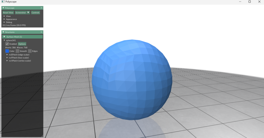
Once the project has been set up, we can begin to test and run our introduction.cu file. If you were to run it, you should get an output of a 3D sphere.
This means the project set up has been successful, we can now begin learning RXMesh.
RXMesh basic workflow
RXMesh provides custom data structures and functions to handle various low-level computational tasks that would otherwise require low-level implementation. Let’s explore the fundamentals of how this workflow operates.
The above is a slightly simplified version of what a for_each computation program would look like using RXMesh. for_each involves accessing every mesh element of a specific type (vertex, edge, or face) and performing some process on/with it.
In the code example above, the computation adjusts the green component of the vertex’s color based on the vertex’s Y coordinate in 3D space.
But how do we comprehend this code? We will look at it line by line:
The above line declares the RXMeshStatic object. Static here stands for a static mesh (one whose connectivity remains constant for the duration of the program’s runtime). Using the RXMesh’s Input directory, we can use some meshes that come with it. In this case, we pass in the dragon.obj file, which holds the mesh data for a dragon.
auto polyscope_mesh = rx.get_polyscope_mesh();
This line returns the data needed for Polyscope to display the mesh along with any attribute content we add to it for visualization.
auto vertex_pos = *rx.get_input_vertex_coordinates();
This line is a special function that directly gives us the coordinates of the input mesh.
auto vertex_color = *rx.add_vertex_attribute<float>("vColor", 3);
This line gives vertex attributes called “vColor”. Attributes are simply data that lives on top of vertices, edges, or faces. To learn more about how to handle attributes in RXMesh, check out this. In this case, we associate three float-point numbers to each vertex in the mesh.
The above lines represent a lambda function that is utilized by the for_each computation. In this case, for_each_vertex accesses each of the vertices of the mesh associated with our dragon. We pass in the arguments:
rxmesh::DEVICE – to let RXMesh know this is happening on the device i.e., the GPU.
[vertex_color, vertex_pos] – represents the data we are passing to the function.
(const rxmesh::VertexHandle vh) – is the handle that is used in any RXMesh computation. A handle allows us to access data associated to individual geometric elements. In this case, we have a handle that allows us to access each vertex in the mesh.
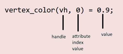
These 3 lines bring together a lot of the declarations made earlier. Through the kernel, we are accessing the attribute data we defined before. Since we need to know which vertex we are accessing its color, we pass in vh as the first argument. Since a vertex has three components (standing for RGB), we also need to pass which index in the attribute’s vector (you can think of it as a 1D array too) we are accessing. Hence vertex_color(vh, 0) = 0.9; which stands for “in the vertex color associated with the handle vh (which for the kernel represents a specific vertex on the mesh), the value of the first component is 0.9”. Note that this “first component” represents red for us.
What about vertex_color(vh, 1) = vertex_pos(vh, 1)? This line, similar to the previous one, is accessing the second component associated with the color, in the vertex the handle is associated with.
But what is on the right-hand side? We are accessing vertex_pos (our coordinates of each vertex in the mesh) and we are accessing it the same way we access our color. In this case, the line is telling us that we are accessing the 2nd positional coordinate (y coordinate) associated with our vertex (that our handle gives to the kernel).
vertex_color.move(rxmesh::DEVICE, rxmesh::HOST);
This line moves the attribute data from the GPU to the CPU.
This line uses Polyscope to add a “quantity” to Polyscope’s visualization of the mesh. In this case, when we add the VertexColorQuantity and pass vertex_color, Polyscope will now visualize the per-vertex color information we calculated in the lambda function.
polyscope::show();
We finally render the entire mesh with our added quantities using the show() function from Polyscope.
Throughout this basic workflow, you may have noticed it works similarly to any other program where we receive some input data, perform some processing, and then render/output it in some form.
More specifically, we use RXMesh to read that data, set up our attributes, and then pass that into a kernel to perform some processing. Once we move that data from the device to the host, we can either perform further processing or render it using Polyscope.
It is important to look at the kernel as computing per geometric element. This means we only need to think of computation on a single mesh element of a certain type (i.e., vertex, edge, or face) since RXMesh then takes this computation and runs it in parallel on all mesh elements of that type.
Writing kernels for queries
While our basic workflow covers how to perform for_each operation using the GPU, we may often require geometric connectivity information for different geometry processing tasks. To do that, RXMesh implements various query operations. To understand the different types of queries, check out this part of the README.
We can say there are two parts to run a query.
The first part consists of creating the launchbox for the query, which defines the threads and (shared) memory allocated for the process along with calling the function from the host to run on the device.
The second part consists of actually defining what the kernel looks like.
We will look at these one by one.
Here’s an example of how a launchbox is created and used for a process where we want to find all the vertex normals:
Notice how, in replacing the for_each part of our basic workflow, we instead declare the launchbox and call our function compute_vertex_normal (which we will look at next) from our main function.
We must also define the kernel which will run on the device.
template <typename T, uint32_t blockThreads>
__global__ static void compute_vertex_normal(const rxmesh::Context      context,
rxmesh::VertexAttribute<T> coords,
rxmesh::VertexAttribute<T> normals)
{


    auto vn_lambda = [&](FaceHandle face_id, VertexIterator& fv){
        // get the face's three vertices coordinates
        glm::fvec3 c0(coords(fv[0], 0), coords(fv[0], 1), coords(fv[0], 2));
        glm::fvec3 c1(coords(fv[1], 0), coords(fv[1], 1), coords(fv[1], 2));
        glm::fvec3 c2(coords(fv[2], 0), coords(fv[2], 1), coords(fv[2], 2));

        // compute the face normal
        glm::fvec3 n = cross(c1 - c0, c2 - c0);

        // the three edges length
        glm::fvec3 l(glm::distance2(c0, c1),
                     glm::distance2(c1, c2),
                     glm::distance2(c2, c0));

        // add the face's normal to its vertices
        for (uint32_t v = 0; v < 3; ++v) {
// for every vertex in this face
            for (uint32_t i = 0; i < 3; ++i) {
// for the vertex 3 coordinates
                atomicAdd(&normals(fv[v], i), n[i] / (l[v] + l[(v + 2) % 3]));
            }
        }
    };

    auto block = cooperative_groups::this_thread_block();

    Query<blockThreads> query(context);
    ShmemAllocator      shrd_alloc;
    query.dispatch<Op::FV>(block, shrd_alloc, vn_lambda);
}
A few things to note about our kernel
We pass in a few arguments to our kernel.
We pass the context which allows RXMesh to access the data structures on the device.
We pass in the coordinates of each vertex as a VertexAttribute
We pass in the normals of each vertex as an attribute. Here, we accumulate the face’s normal on its three vertices.
The function that performs the processing is a lambda function. It takes in the handles and iterators as arguments. The type of the argument will depend on what type of query is used. In this case, since it is an FV query, we have access to the current face(face_id) the thread is acting on as well as the vertices of that face using fv.
Notice how within our lambda function, we do the same as before with our for_each operation, i.e., accessing the data we need using the attribute handle and processing it for some output for our attribute.
Outside our lambda function, notice how we need to set some things up with regards to memory and the type of query. After that, we call the lambda function to make it run using query.dispatch
Visualizing face normals
Now that we’ve learnt all the pieces required to do some interesting calculations using RXMesh, let’s try a new one out.
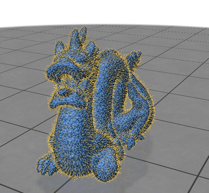
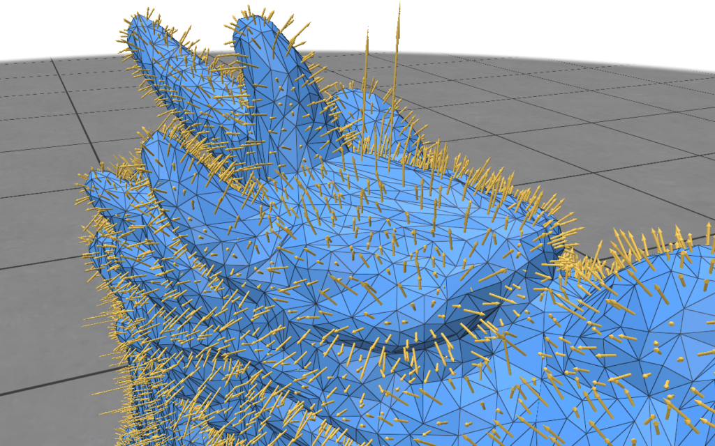
Try to visualize the face normals of a given mesh. This would mean obtaining an output like this for the dragon mesh given in the repository:
Here’s how to calculate the face normals of a mesh:
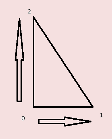
Take a vertex. Calculate two vectors that are formed by subtracting the selected vertex from the other two vertices.
Take the cross product of the two vectors.
The vector obtained from the cross product is the normal of the face.
Now try to perform the calculation above. We can do this for each face using the vertices it is connected to.
All the information above should give you the ability to implement this yourself. If required, the solution is given below.
The kernel that runs on the device:
template <typename T, uint32_t blockThreads>
global static void compute_face_normal(
const rxmesh::Context context,
rxmesh::VertexAttribute coords, // input
rxmesh::FaceAttribute normals) // output
{
auto vn_lambda = [&](FaceHandle face_id, VertexIterator& fv) {
    // get the face's three vertices coordinates

    glm::fvec3 c0(coords(fv[0], 0), coords(fv[0], 1), coords(fv[0], 2));
    glm::fvec3 c1(coords(fv[1], 0), coords(fv[1], 1), coords(fv[1], 2));
    glm::fvec3 c2(coords(fv[2], 0), coords(fv[2], 1), coords(fv[2], 2));

    // compute the face normal
    glm::fvec3 n = cross(c1 - c0, c2 - c0);
    normals(face_id, 0) = n[0];
    normals(face_id, 1) = n[1];
    normals(face_id, 2) = n[2];
};

auto block = cooperative_groups::this_thread_block();
Query<blockThreads> query(context);
ShmemAllocator shrd_alloc;
query.dispatch<Op::FV>(block, shrd_alloc, vn_lambda);

}
Color a vertex depending on how many vertices it is connected to.
Test the above on different meshes and see the results. You can access different kinds of mesh files from the “Input” folder in the RXMesh repo and add your own meshes if you’d like.
By the end of this, you should be able to do the following:
Know how to create new subdirectories in the RXMesh Fork
Know how to create your own for_each computations on the mesh
Know how to create your own queries
Be able to perform some basic geometric analyses’ using RXMesh queries
This blog was written by Sachin Kishan during the SGI 2024 Fellowship as one of the outcomes of a two week project under the mentorship of Ahmed Mahmoud and support of Supriya Gadi Patil as teaching assistant.