Or how to figure out the right way to skin a cat (for texture mapping)
By: Kirby Dietz and Bonnie Magland, mentored by Yusuf Sahillioglu
Introduction:
For the past two weeks, we have been doing research on how to optimize making 2D cuts onto a surface such that we get an optimal parameterization of the surface onto a disk. This question more generally is asking how we can take a triangulated surface and perform operations on it such that we see a representation of this surface on a disk that we can apply texture mapping or other various changes to.
Firstly let us explain why we want to make these cuts. We make these cuts so that we can use existing methods of disk parameterization from a surface with a boundary onto a disk. We can also think about making a 2D surface from our 3D surface using cuts in a more intuitive way. We can think about it like how a net works, that we know it is true that if we took enough cuts it would be true that we get a locally distortion free 2D representation of the surface; however doing this would both be computationally intensive and not very useful for performing tasks that we want, such as texture mapping, and it does not give an intuitive understanding of what the general surface is or what each section of the 2D map corresponds with each section of the surface. Thus the question becomes how do we take a minimal amount of cuts such that we have a 2D parameterization of the surface that minimizes distortion such that we can still use it for various texture mapping applications.
Disk Parameterization:
First we worked on mapping 3D meshes with existing boundaries to a disk. We implemented existing methods of disk conformal parameterization using three different weight functions. We start by mapping the mesh boundary to the circle, preserving the distance between chord edges. Placing the interior points is then a matter of solving a system of linear equations. In our first weighting method, each edge is weighted the same so in the resulting disk, interior points are the centroid of their neighbors. This gives one linear equation for each interior point, and since the boundary points are fixed, we can solve for the exact locations of each point on the disk.
Weighing each edge uniformly results in unnecessary distortion. Our second and third methods use the angles in the faces sharing the edge to add weights to the equations in the first method. The second method uses harmonic weights, with formula \(w_{i,j}=\frac{1}{2}\left( cot(i,j) + cot(i,j)\right)\) where \(\alpha_{i,j}\) and \(\beta_{i,j}\) are the angles opposite the edge connecting the \(i\) and \(j^{th}\) vertices. These weights reduce distortion, but obtuse angles can result in negative weights, so the resulting map is not guaranteed to be bijective. The third method, mean value weights, resolves this by instead using \(w_{i,j}=\frac{tan(\frac{\gamma_{i,j}}{2}) + tan(\frac{\delta_{i,j}}{2})}{2|| v_i – v_j ||}\) where \(\gamma_{i,j}\) and \(\delta_{i,j}\) are the angles adjacent to the edge connecting the \(i\) and \(j^{th}\) vertices. In our future disk parameterizations, we use these last two methods.
Virtual Boundary:
A downside to disk parametrization is that because the boundary has a fixed mapping to the circle, the resulting parameterization has a lot of distortion near the perimeter. There are a variety of free-boundary parameterization methods, but we focused on the virtual boundary method. By adding one or more layers of faces to the existing boundary, we create a new, virtual boundary that is mapped to the circle while the real boundary is allowed a less constrained shape. We can then ignore the added faces and use the resulting parameterization. The more layers in the virtual boundary, the more “free” the resulting boundary. For example, the mountain range mesh below has a boundary that is more rectangular in shape than circular. As we add more layers to the virtual boundary parameterization, we can see the outline become more square as well.

 |  |  |
| 1 Layer | 5 Layers | 10 Layers |
However, it is not always necessary to add multiple layers, but instead simply increase the size of the virtual boundary, this is due to how the virtual boundary is created following the method used in “Parametrization of Triangular Meshes with Virtual Boundaries” by Yunjin Lee, Hyoung Seok Kim, and Seungyong Lee. We create the virtual boundary by listing the vertices in the existing boundary as \(v_1,v_2,\dots,v_n\) and label the vertices in the virtual boundary \(v’_1,v’_2,\dots,v’_{2n}\) where \(v_i\) corresponds to \(v’_{2i}\), we then make sure the distance between \(v_i , v_{i+1} \) proportional to the distance between \(v_{2i} , v_{2i+2}\) and assigning \(v_{2i+1}\) to the midpoint between the two, to do this we simply say that \(v_{2i}=av_i\). Thus we can increase the size of the virtual boundary simply by increasing the a value, this allows a quicker method of getting a virtual boundary that gives the same results as running multiple layers of virtual boundaries.

 |  |
| a = 1.05 | a = 1.5 |
Many meshes that we want to parameterize in 2D do not have boundaries. In order to do this, we make a cut along existing edges in the mesh to create our own boundary. A cut can be visualized as exactly how it sounds—taking a pair of scissors and slicing through the mesh. It is created from a path of edges by duplicating the non-endpoint vertices in the path, and connecting them to create a loop of boundary edges. This connected loop will naturally form by reassigning the faces on one side of the path to contain the new vertices rather than the old duplicated vertices.
The trouble comes with determining which side of the cut each face is on. We created our own cutting algorithm, and solved this problem by using the orientation of the faces with edges on the path. Given a directed path, the faces with edges on one side of the path will be oriented in the direction of the path, while the faces on the other side will be oriented in the opposite direction. Thus we can easily separate the faces sharing edges along the cut. A more difficult task is separating the faces that only share one vertex with the cut path. To solve this quickly, we store the directions of edges coming from each point on the path that are confirmed to be on one side of the path. We then can determine which side of the path a face is based on how close its edges’ direction is to these edges. There are conceivable shares which will cause this to fail, but in practice this can quickly implement the vast majority of cuts.
We also tried a different algorithm to determine which side of the cut each face is on, making use of geometric properties of the surface, in specific the normal of the surface. We compared the normal of the face to the normal of the edge on the cut. We took the plane defined by the normal on the cut, and compared if the normal of the face projected onto the plane was on the left or right of the plane, when considering the y-axis of the plane to be the edge. This result showed initial success, and continuous to work along small cuts, or cuts along areas of low curvature, however when dealing with areas of large curvature the cut has a large issue, that is when the surface has high curvature it is possible for the edge to be behind the surface with respect to where the edge is, which gives the normal on the other side than we desire, and thus gives it to be on the right when it is on the left, and other such issues, for this reason we have discarded this approach, however we are open to the possibility that using some operation on the normals it might be possible to use this approach.
Euclidean Max Cut:
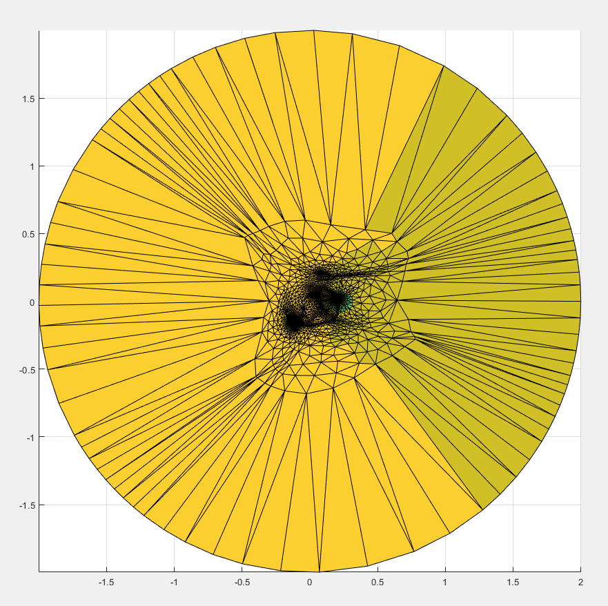
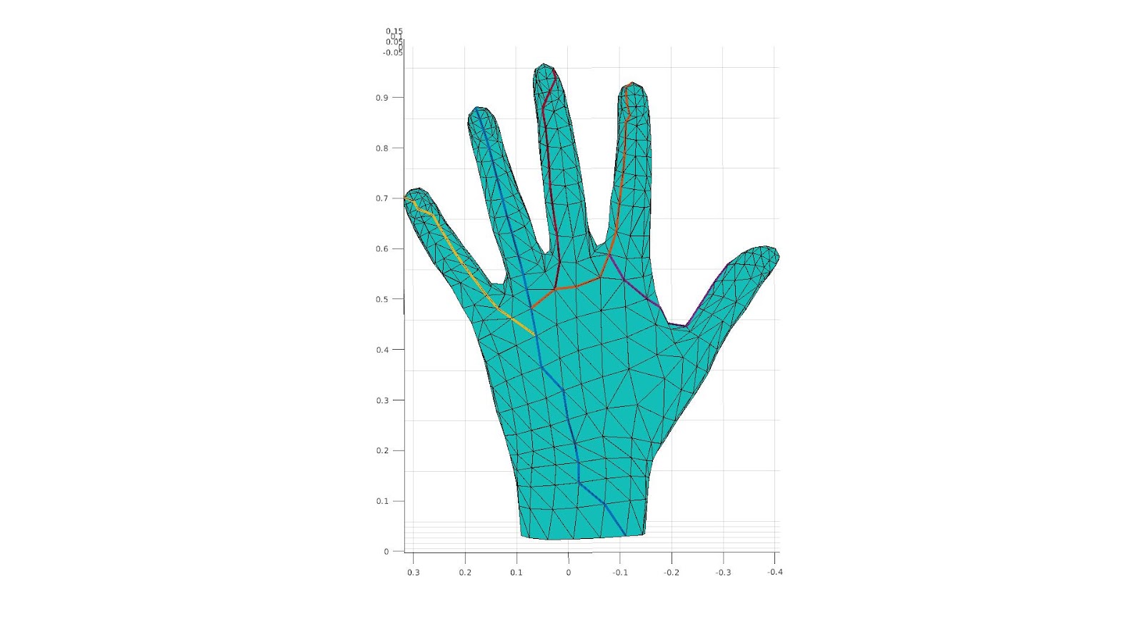
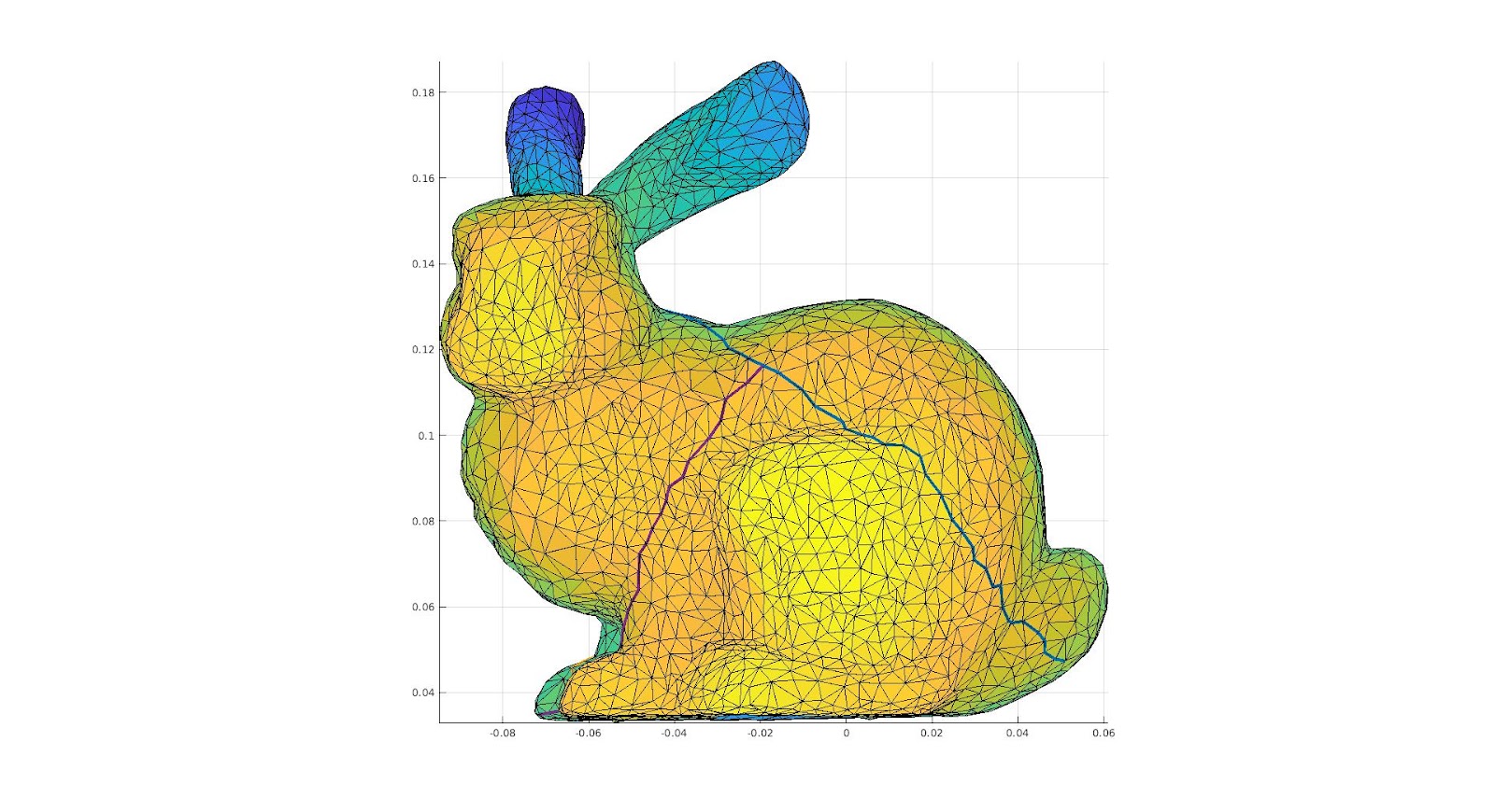
Now let us discuss our main method of how to choose a cut to make, we considered existing methods, namely the method of using a minimal spanning tree as used by Alla Sheffer in “Spanning Tree Seams for Reducing Parametrization Distortion of Triangulated Surfaces,” seemed to have the opposite desire than we want, that is, to minimize the size of the cut. It is clear simply from the boundaries we were provided as well as intuition that the larger the cut the smaller the distortion would be, as if we had a large enough cut there would be no distortion, however we also know that artifacts exist along the cuts, thus we created a new method. This method was a way of maximizing the distance of the cut while minimizing the artifacts. This was maximizing the Euclidean distance between the end points of the path of the cut while making the cut that takes the minimum geodesic distance.
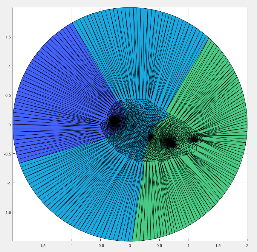
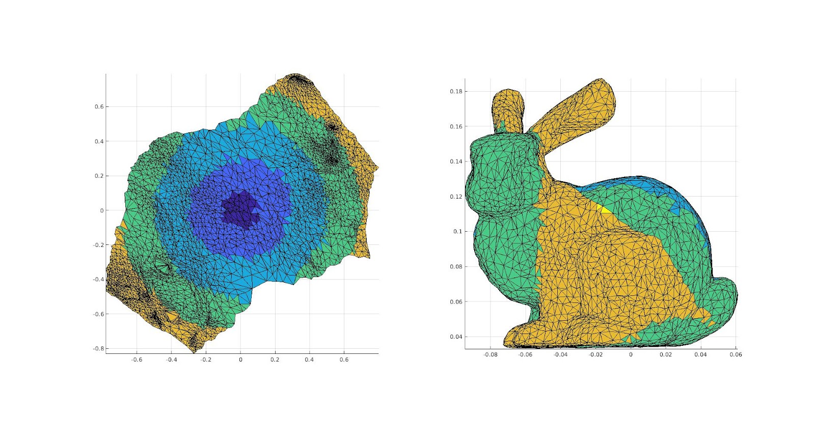
 |  |  |
| The surface, and the cut we are making upon it. | A color function we add to the surface in order to see where different areas are mapped onto a 2D Parameterization. | The 2D Parameterization with Virtual Boundary. |
 |  |  |
| The surface, and the cut we are making upon it. | A color function we add to the surface in order to see where different areas are mapped onto a 2D Parameterization. | The 2D Parameterization with Virtual Boundary. |
 |  |  |
| The surface, and the cut we are making upon it. | A color function we add to the surface in order to see where different areas are mapped onto a 2D Parameterization. | The 2D Parameterization with Virtual Boundary. |
 |  |  |
| The surface, and the cut we are making upon it. | A color function we add to the surface in order to see where different areas are mapped onto a 2D Parameterization. | The 2D Parameterization with Virtual Boundary. |
As we can see however this creates unintuitive cuts, and cuts that do not have our desired purpose, for this we considered a new method of cuts.
Medial Mesh Max Cut:
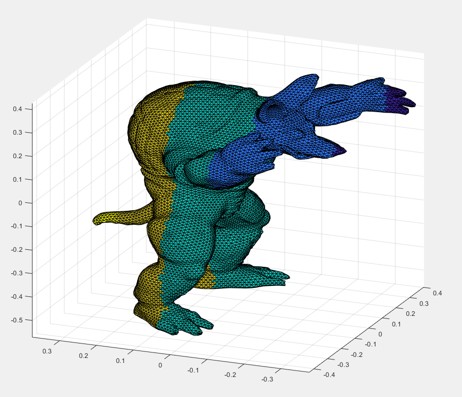
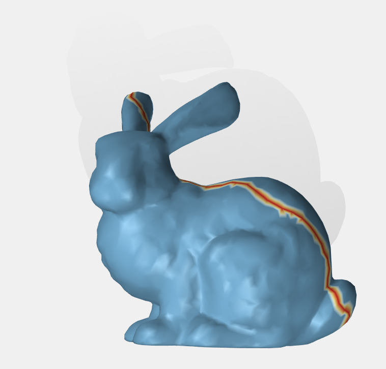
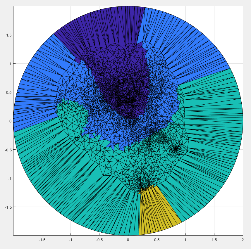
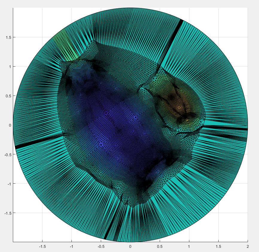
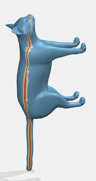
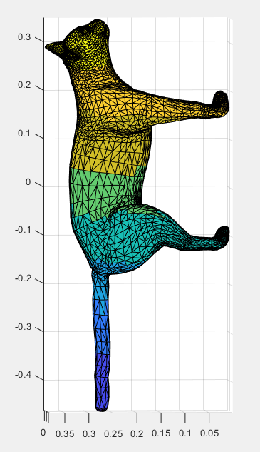
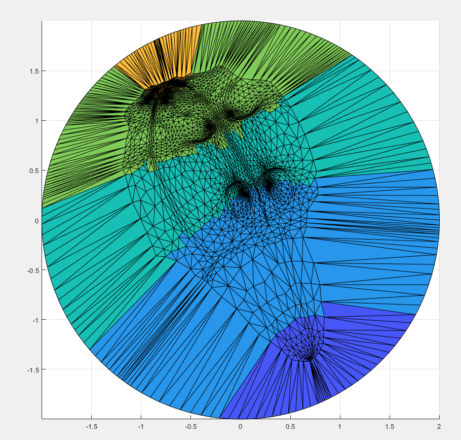
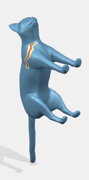
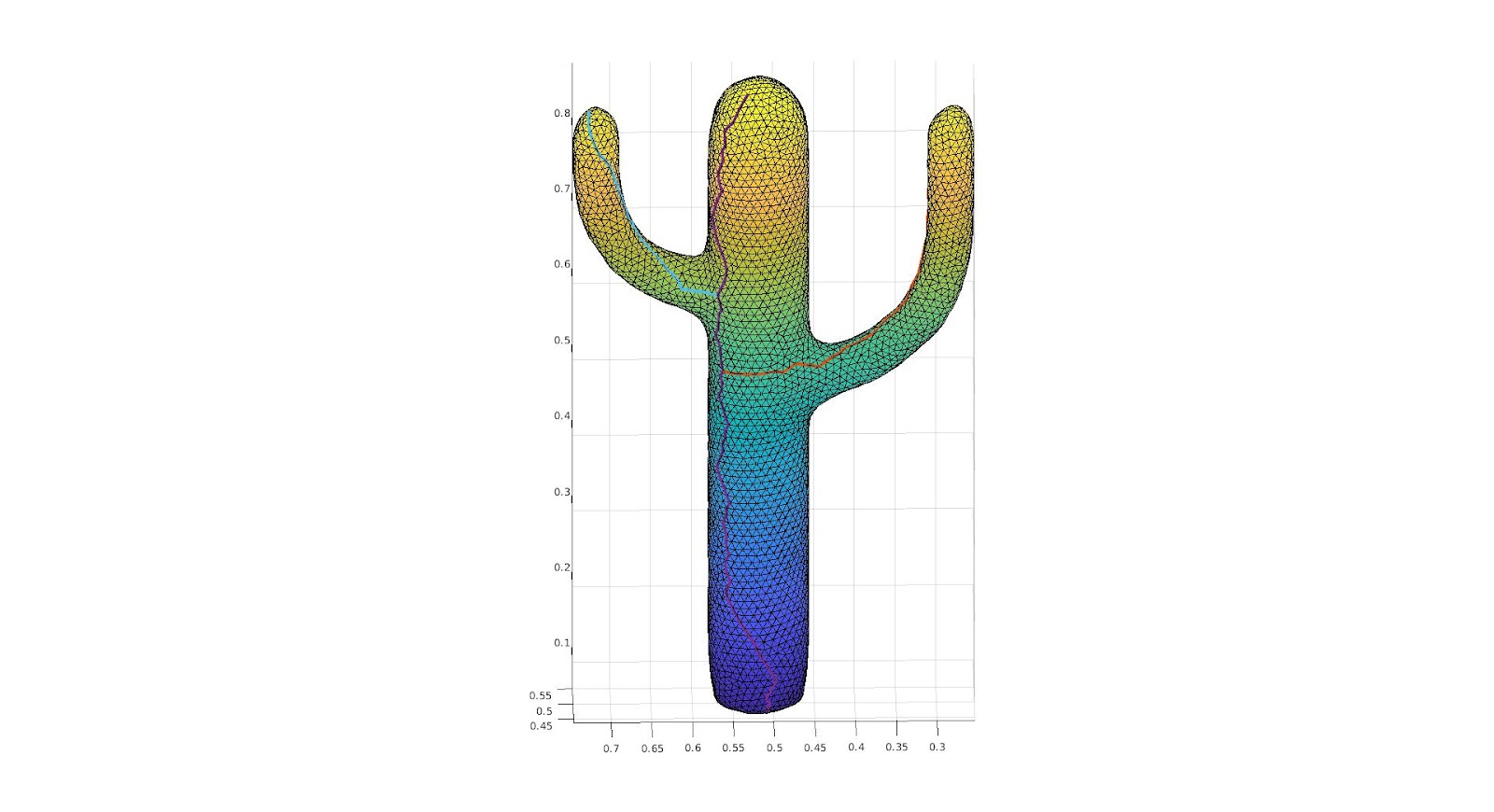
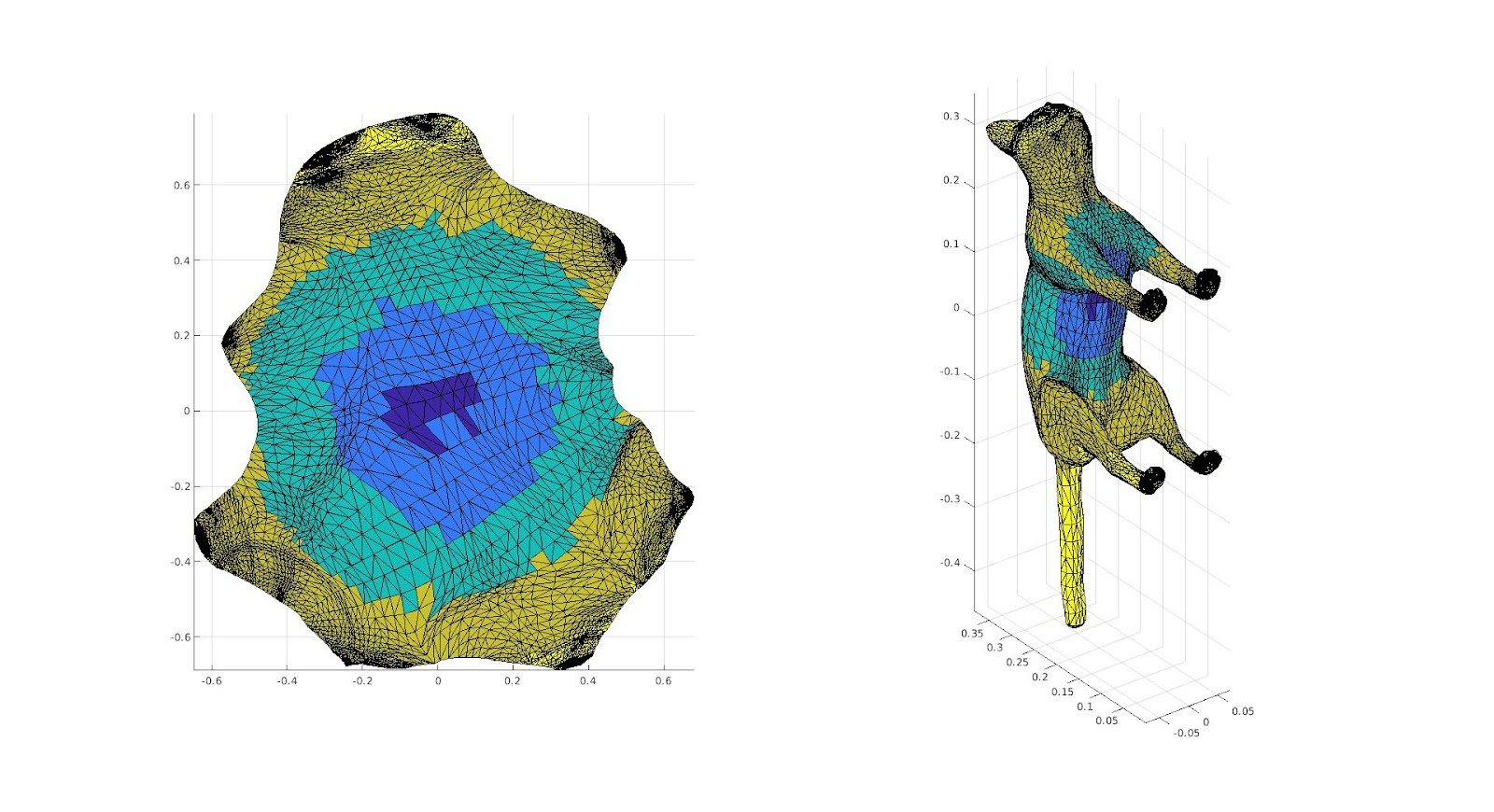
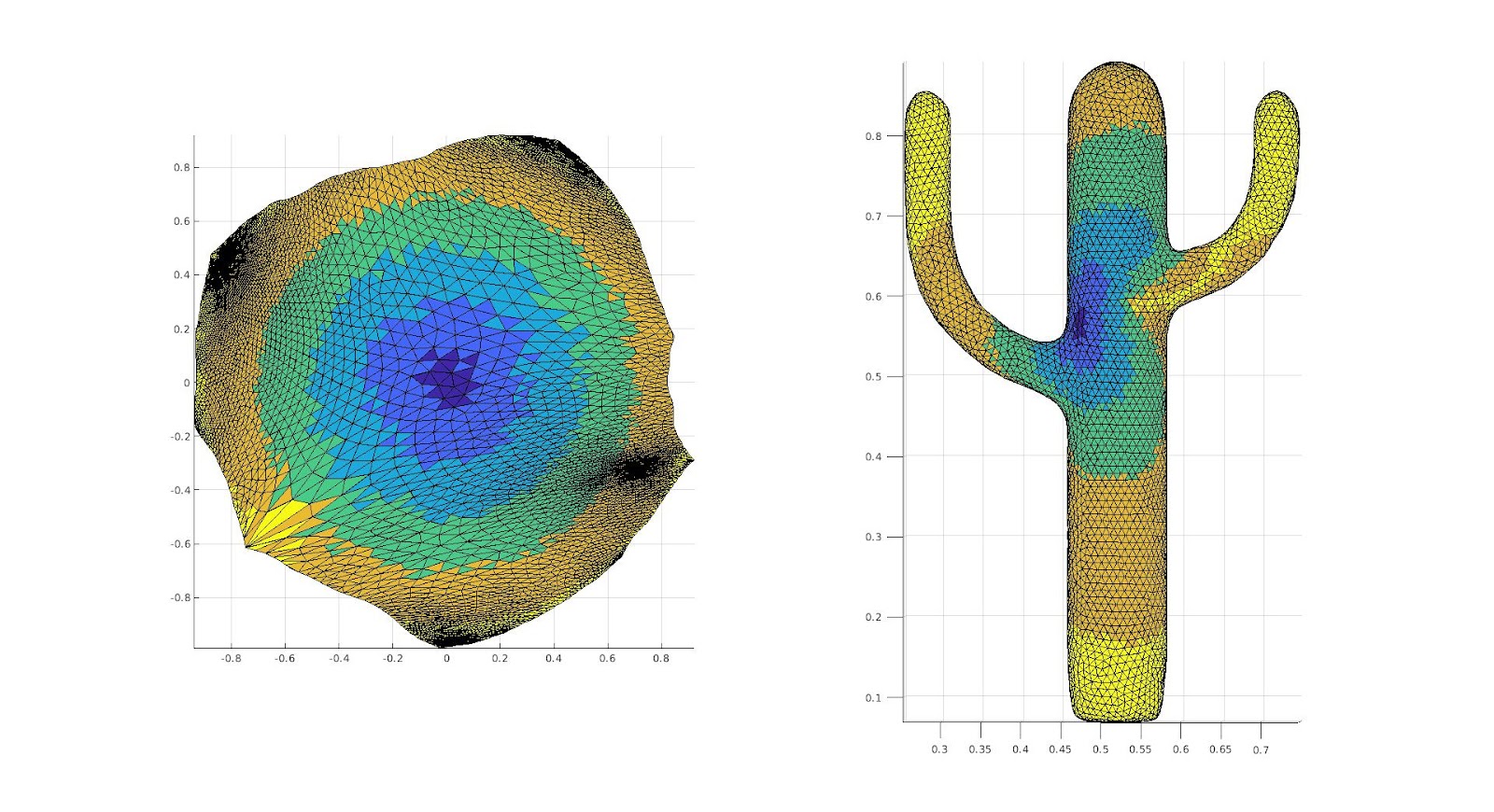
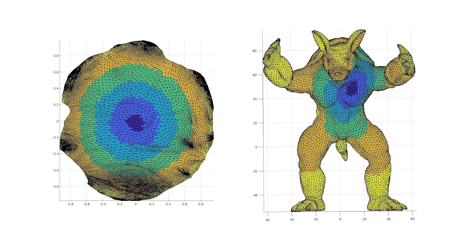
To deal with this issue, we implemented a new method using the medial mesh, that is we consider a simplified mesh of the object making use of the midpoints of the faces within the interior of the surface. We did not do implementation of finding this medial mesh ourselves, rather using the code created in “Q-MAT: Computing Medial Axis Transform by Quadratic Error Minimization” by Pan Li, Bin Wang, Feng Sun, Xiaohu Guo, Caiming Zhang and Wenping Wang. We then after obtaining the Medial Mesh, create the minimal spheres on each vertex, that is the smallest sphere with the center at a vertex in the medial mesh, such that it intersects with a vertex on the surface. We then created a graph with vertices representing the spheres, and creating an edge if the spheres overlap, we then calculated the maximum path existing on the graph, with the edge lengths equal to the distance between the center of the spheres. We then identified the vertices on the surface such that they were the closest to the points on each sphere such that the Euclidean distance between the two end point spheres is maximized, we use these as the two points to create a cut on and we create a cut with the minimum geodesic distance between the two points. This was hopefully to avoid areas of high curvature, and thus create a better cut still of a reasonably large size.
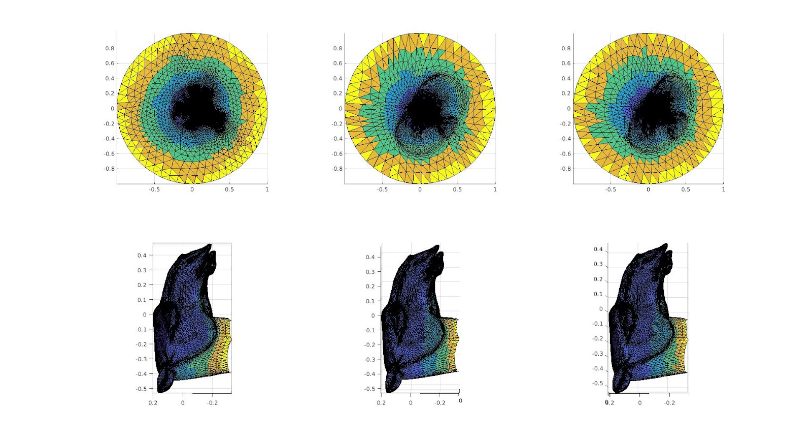
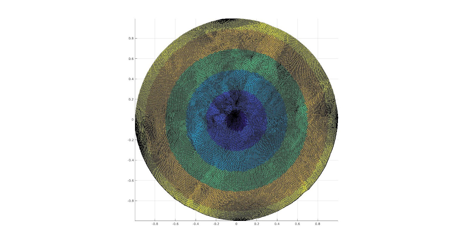
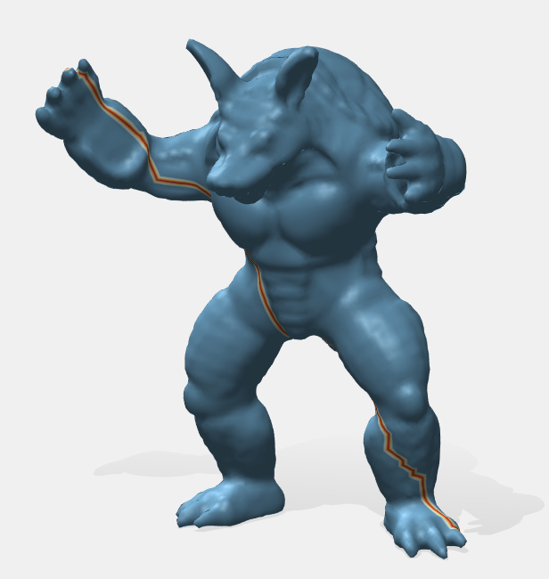
 | 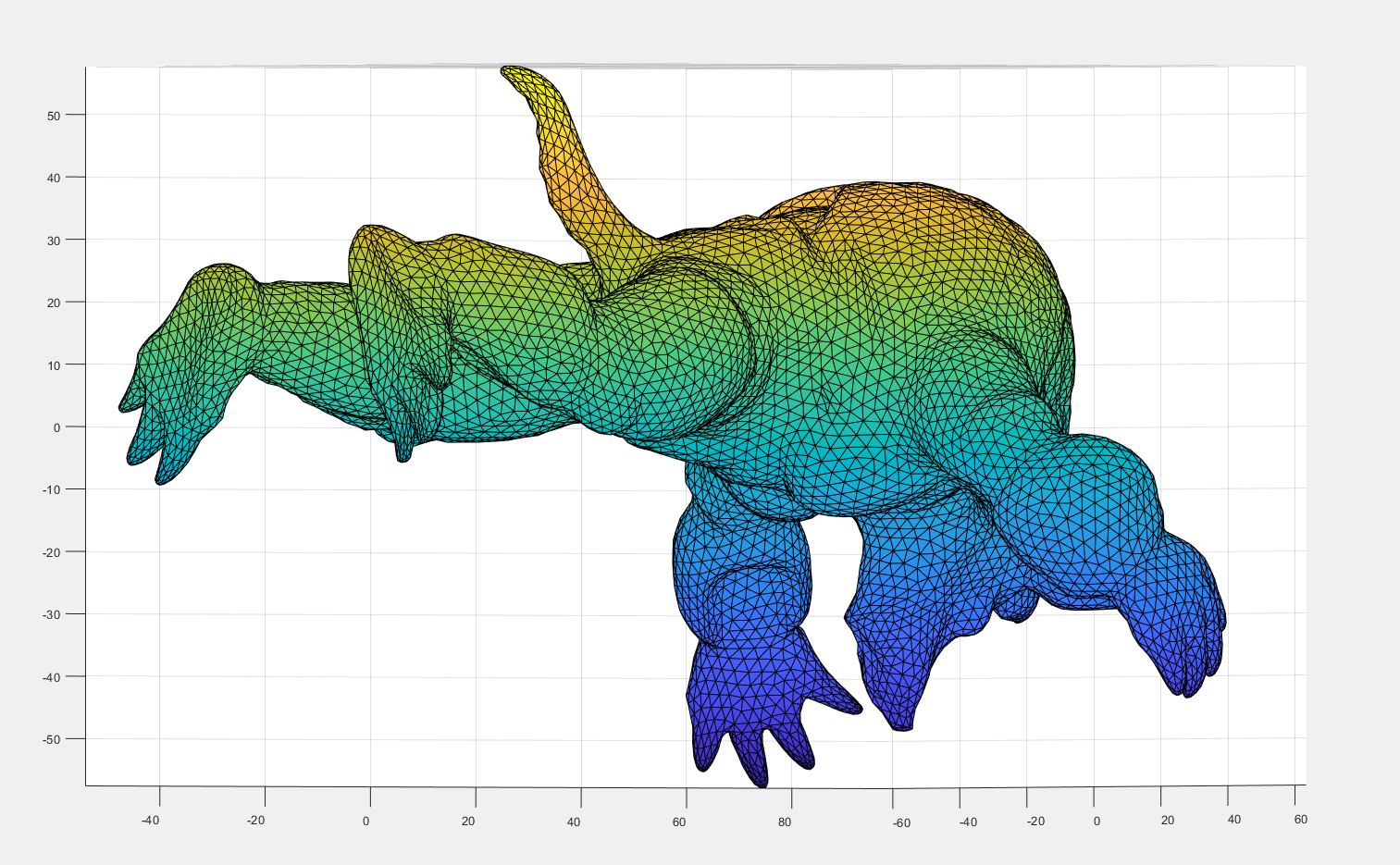 | 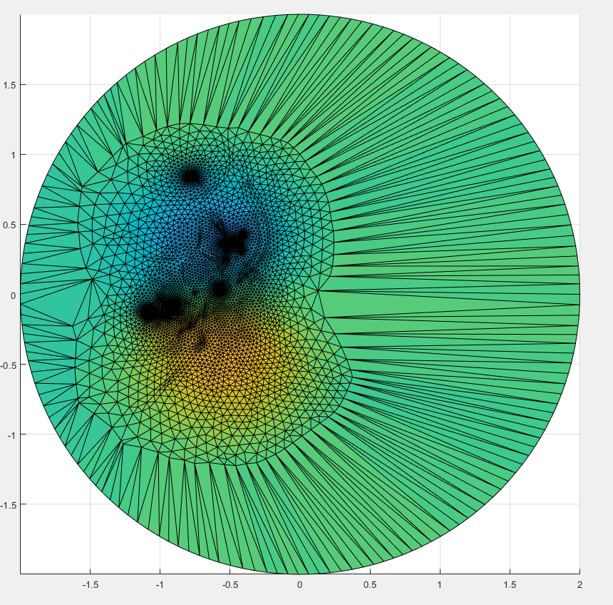 |
| The surface, and the cut we are making upon it. | A color function we add to the surface in order to see where different areas are mapped onto a 2D Parameterization. | The 2D Parameterization with Virtual Boundary. |
 | |  |
| The surface, and the cut we are making upon it. | A color function we add to the surface in order to see where different areas are mapped onto a 2D Parameterization. | The 2D Parameterization with Virtual Boundary. |
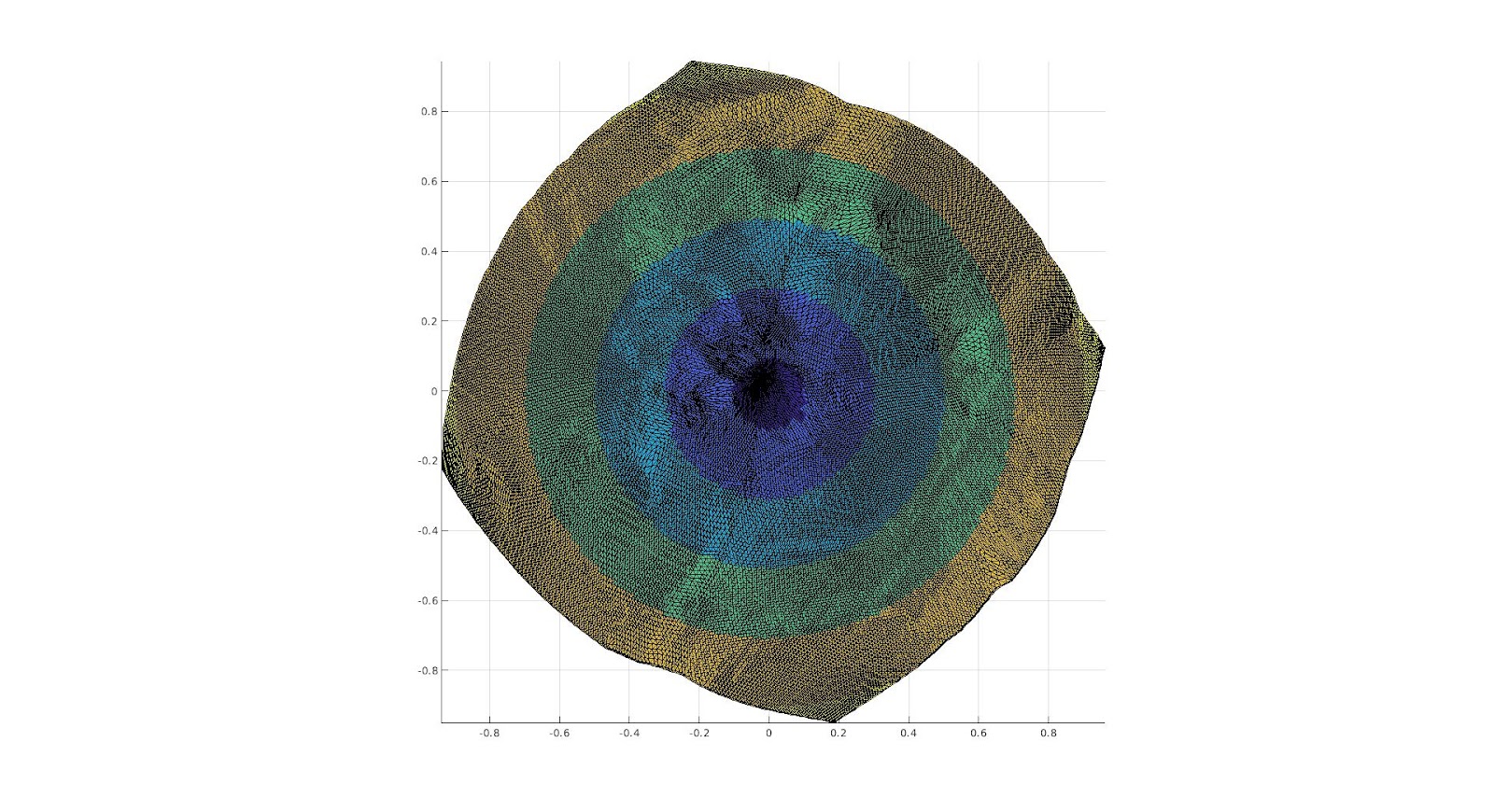
 |  |  |
| The surface, and the cut we are making upon it. | A color function we add to the surface in order to see where different areas are mapped onto a 2D Parameterization. | The 2D Parameterization with Virtual Boundary. |
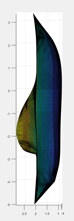
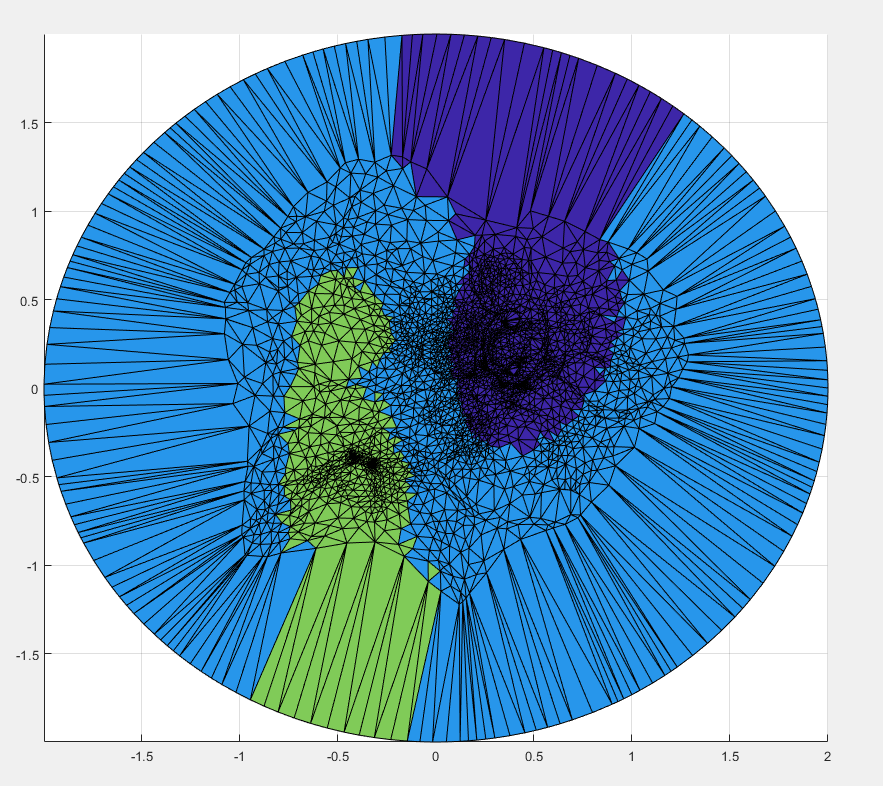
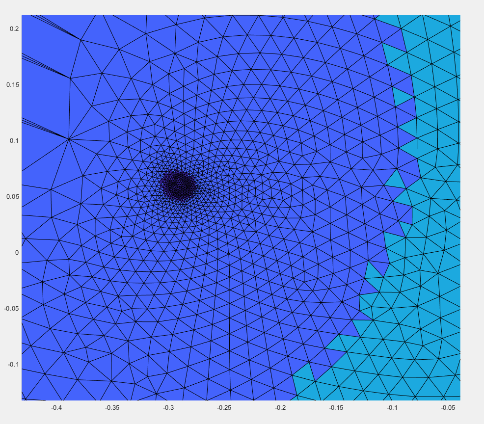
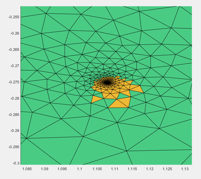
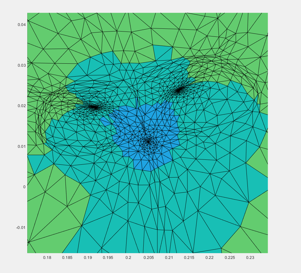
Of note is that areas that are not on the cut area directly are “tucked in” so to into the areas that we can barely see. The one below is in the left area with a high density of vertices. The rest follow from left to right the areas of high vertices.
 |  |  |  |
 | |  |
| The surface, and the cut we are making upon it. | A color function we add to the surface in order to see where different areas are mapped onto a 2D Parameterization. | The 2D Parameterization with Virtual Boundary. |
We again get areas of high curvature being sort of tucked into the surface.
 |  |
| The bottom left area that shows the face. | The right middle area showing the back legs and tail. |
How Multiple Cuts work:
Thus far we have only discussed and shown single cuts along simple paths. It is also possible, and often preferred, to make multiple cuts on intersecting paths. Making these cuts sequentially, each new cut is equivalent to making a cut on a shape that already has a boundary. If the cut path has one endpoint on the boundary and the rest of the points on the interior, then the resulting boundary is still a simple closed path, as is necessary for our 2D parameterization. The method is the same as before, except the endpoint on the existing boundary is duplicated in addition to the other points. Using multiple cuts increases the freedom of our cut paths and allows us to cut along branching pieces of a mesh.
We can extend our previous Euclidean maximum cut method to multiple cuts in an iterative process. After making our first cut as usual, we repeat the same method but restricting one of the endpoints to be on the previous cuts. Our second cut selects the point that is farthest from our new boundary and chooses the shortest path between them. This is repeated until there are the desired number of cuts. Below are some examples of multiple cuts using this method. One possible automated method of stopping would be to calculate the standard deviation of the distance from the boundary and continue to create cuts until it is below some threshold.
 |  |
| The surface, and the cuts we are making upon it. | The 2D Parameterization and a color function that we take from 2D parameterization to the surface. |
 |  |
| The surface, and the cuts we are making upon it. | The 2D Parameterization a color function that we take from 2D parameterization to the surface. |
 |  |
| The surface, and the cuts we are making upon it. | The 2D Parameterization a color function that we take from 2D parameterization to the surface. |
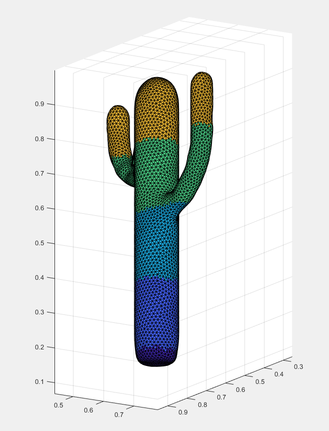
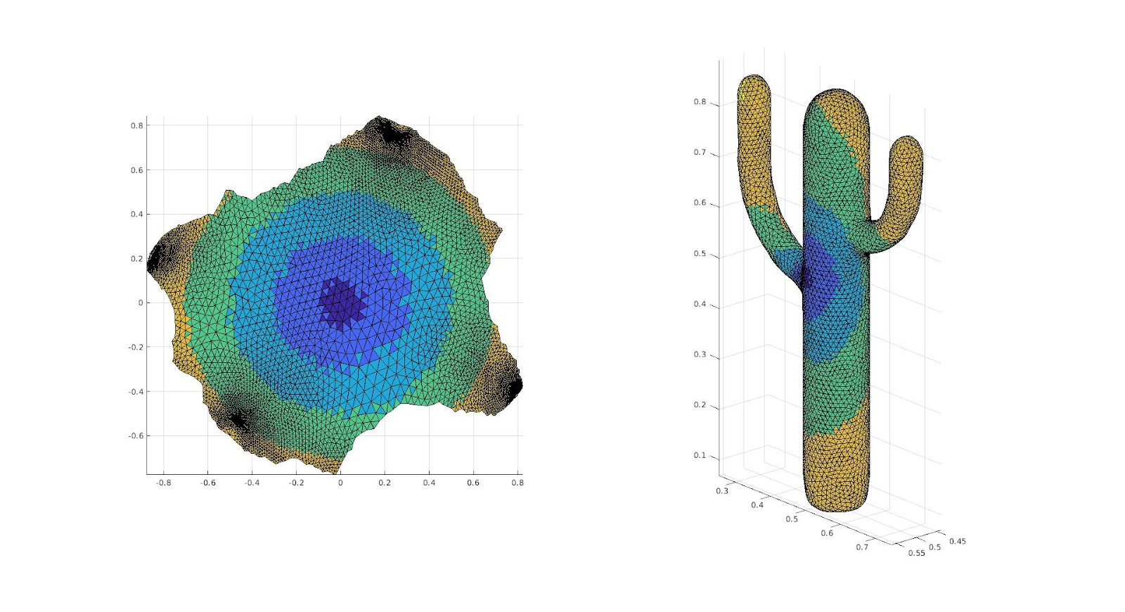
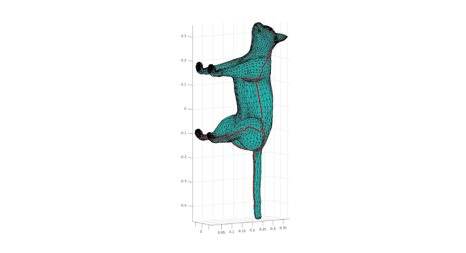
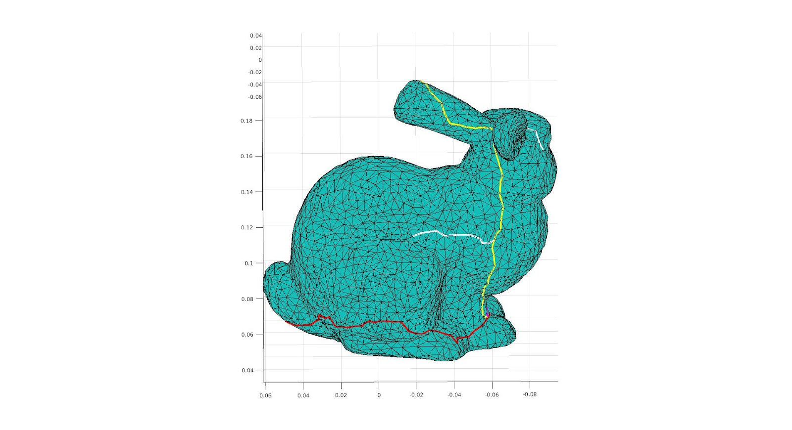
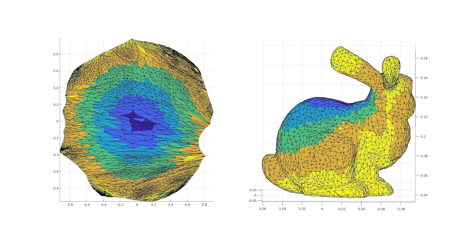
We can also use the sphere approximation to make multiple cuts. The spheres’ centers indicate important spots in the mesh, like joints and protrusions. We decided to use a minimum spanning tree to determine a sequence of cuts that connects each of these areas. First we project each sphere center to a vertex on the mesh. Then we make a weighted graph out of these points where an edge between two points is weighted as their geodesic distance. This graph gives a minimum spanning tree that can be broken into a sequence of cut paths that connects each point from our sphere approximation. The paths sometimes require simple adjustments to remove overlap, and then they are ready for our cutting algorithm.
 |  |
| The surface, and the cuts we are making upon it. | The 2D Parameterization a color function that we take from 2D parameterization to the surface. |
 |  |
| The surface, and the cuts we are making upon it. | The 2D Parameterization a color function that we take from 2D parameterization to the surface. |
 |  |
| The surface, and the cuts we are making upon it. | The 2D Parameterization a color function that we take from 2D parameterization to the surface. |
 | |  |
| The surface from the front, and the cut we are making upon it. | The surface from the back, and the cuts we are making upon it. | The 2D Parameterization a color function that we take from 2D parameterization to the surface. |
Conclusion:
This research was very interesting, but we did not get the sort of success that we would like: While we did get surfaces with minimal distortion, specifically those with multiple cuts, we did not get the desired usage that we would like. Thus it is necessary to state what future direction should be taken if this research would be continued. There are three main areas for future work.
The first is making cuts along lines that preserve symmetry, that is if the surface has symmetry along some axis, or some feature, the 2D parameterization also has these symmetries. This would be useful both for minimizing the distortion and would provide intuitive results for texture mapping. These lines of symmetry, however, would be incredibly difficult to calculate, so we would like for them to be usually user specified, which brings us to the second area: how the inclusion of landmark areas would be useful, that is specifying areas where the cut cannot travel through. This allows us to intuitively avoid areas of high curvature that are important to the surface and how it could be applied to different surfaces as useful for an artistic application.
We could also try to do this in an automated way by using a skeletal approximation of the surface, using either a simplified medial mesh or a method presented in the SGP 2021 Graduate School Course Shape Approximations & Applications: using the sphere mesh proxy simplification of a surface. This method considers the edges between the spheres as the “bones” and makes a cut on each bone section such that it goes over the entirety of the bone, but avoids areas of high curvature by making minimal geodesic cuts along each bone; the method connects the bones by paths the minimize the total geodesic distance. A secondary way to use this is to make cuts along the “bones” but additionally taking a cut perpendicular to the bone at each point where the sphere begins. To think of this on a 3D model of a cat, for example, we would take a cut along the spine, and then take a perpendicular cut along the cat. To see if either of these methods work and if so which is better, further research would be needed.