Bryce – SGI 2021

AKA: Takeaways from Weeks 1-2 of High-order Directional Field Design Research

Author: Bryce Van Ross

It’s incredible how much one can learn in a month, and I’m looking forward to learning more (especially theoretically). In that same spirit, I highlight some takeaways from research made in my first SGI project. This project was guided by research mentor Dr. Amir Vaxman and TA Klara Mundilova, where I worked with fellow SGI student Jonathan Mousley.

Question(s): Usually we think of vectors and computations like divergence and curl as interrelated, and they are. But can we determine something more nuanced about these properties with respect to some vector field if we encounter a complex (i.e. having multiple vertices/edges) triangular mesh? Yes, we can. But it depends on your choice of approach of partitioning your mesh. For the sake of my research, we focus on the face-based representation.

Face-based representations of vector fields can then be broken down into vertex-based and edge-based approaches, per face per triangle. This means we are working with vector fields on faces that are gradients of (piecewise linear) functions that are either defined on the vertices or on the midpoints of edges. Depending on the choice of approach, then your computations are different. But which way is better and what are the consequences?

Answer(s): This is a natural question. Vertex-based (for certain reasons) seems to yield better approximations, which lead to better attempts at mimicry of continuity. In this sense, vertex-based computations are considered conforming, whereas edge-based computations are deemed nonconforming (w.r.t. continuity). Suppose we wanted to express a given vector field u in terms of familiar computations. Naturally, we would prefer to use vertex-based computations. However, we must remember that degrees of freedom (D.O.F.) must be maintained. Surprisingly, using purely vertex-based computations (or, purely edge-based computations) are in violation of D.O.F. More surprisingly, we find that our only solution is to use a mix of both the conforming and nonconforming terms. So, even though the gradients are distinct, both are equally valuable in terms of a reduction of u. So, there is a need to incorporate both \(G_v\) (the vertex-based gradient) and \(G_e\) (the edge-based gradient). This mixture could be complicated, but isn’t…it only requires the sum of 3 terms. The first term includes \(G_v\) and computes the divergence but is curl-free. For the second term, including \(G_e\), it computes the curl yet is div-free. The last term, referred to as \(h\), is both divergence-free and curl-free. Note: that \(G_v\) and \(G_e\) can be interchanged w.r.t. the first two terms if such equation is multiplied by the rotation matrix \(J\). Ultimately, u (or any vector space) has non-trivial representation (a.k.a. there’s more than meets the eye).

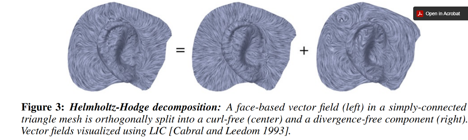
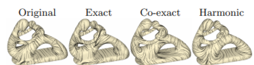
There’s more to it, but the above refers to the Helmholtz-Hodge Decomposition: \[u = G_v\cdot f + J\cdot G_e\cdot g + h.\] A better visualization can be found below (Source: Vector Field Processing on Triangle Meshes), where the h term is not illustrated, in the topmost picture below. In the secondary picture, all components are expressed (Source: Subdivision Directional Fields, Figure 9, Top Row).

Author: Bryce Van Ross

Currently, we’re finishing the first half of the 2-week Robust computation of the Hausdorff distance between triangle meshes project. This research is lead by mentor Dr. Leonardo Sacht, TA Erik Amézquita, and in my immediate team, I work with fellow students Deniz Ozbay and Talant Talipov. The below is a brief summary of what’s happened so far:

A mathematical visualization of the Hausdorff distance of two meshes

Source: https://en.wikipedia.org/wiki/Hausdorff_distance

Applications: Primarily computer vision, computer graphics, digital fabrication, 3D-printing, and modeling. For example, in computer vision, it is often desirable to identify a best-candidate target relative to some initial template. In reference to the set of points within the template, the Hausdorff distance can be computed for each potential target. The target with the minimum Hausdorff distance would qualify as being the best fit, ideally being a close approximation to the template object.

Motivation: Objects are geometrically complex. There are different ways to compare objects to each other via a range of geometry processing techniques and geometric properties. Distance is often a common metric of comparison. But what type of distance should we use, which distances are favorable, and why? These are important questions.

Pitfalls of using other types of distance for triangular meshes

Source: http://cgm.cs.mcgill.ca/~godfried/teaching/cg-projects/98/normand/main.html

For our research, we focus on computing the Hausdorff distance \(h\). “Hausdorff” may seem familiar to you if you know topology. There, a (topological) space is considered Hausdorff if any two elements can be separated into disjoint (open) sets. The key idea here is the separation property with respect to points.

In geometry processing, this idea is extended (in some sense) to the separation of triangle meshes. The Hausdorff distance \(h\) is fundamentally a maximum distance among desirable distances between 2 meshes. These desirable distances are minimum distances of all possible vectors resulting from points taken from the first mesh to the second mesh. But why is \(h\) significant? If \(h\) converges to zero (the smallest possible distance), then this implies that our meshes, and therefore the objects themselves, are very similar. This, like most things in math, implies within some epsilon, representing marginal change such as a slight deformation, rotation, translation, compression, or stretch. If \(h\) is large, then this implies that the two objects are dissimilar. Intuitively, this is due to a lack of ideal correspondence from triangle to triangle. In short, \(h\) serves as a means of computing the similarity between digital objects in terms of maximally separating the meshes’ points according to their minimum distances.

Tasks: To compute \(h\), we find the maximizer, the point (in the first mesh) corresponding to the computation of \(h\). This point is found via an algorithmic process called the branch and bound technique. Sparing the details, the result of applying this technique will provide a (very small) region where the minimizer is claimed to exist, after a series of triangle subdivisions and deletions. There are different ways to implement this technique. Our collective goal this week was to achieve accurate \(h\) given any two meshes. Once this is ensured, Week 2 would focus on making our code more robust (efficient/fast). This work can be simplified into three primary tasks: encoding the lower bound and upper bound of possible values of \(h\), and the subdivision method. My work focused on the lower bound, for which the other two functions are dependent.

Accomplishments: By Day 2, we started with writing pseudocode for the lower bound, using only the vertices of the first mesh and computing their distances with respect to vertices of the second mesh. This was computed per face, and the minimum was found. Although this method was correct, it didn’t account for either the edge or interior cases of a given triangle. Looping through an edge would be immediately doable, but the interior case would be more challenging. Thankfully, Dr. Sacht had us search through gptoolbox for such functionality that would account for all three cases. Once finding this function, we were able to reduce my code to two lines! The irony is although this was valid, the referenced function was basically an empty shell. The function was actually calling a C++ function that would have to compiled and linked against other libraries and due to our time constraints we decided it was best to address this issue in a future time. Ultimately, we ended up having to write from scratch once more. In searching for similar point-triangle distance algorithms, we initially found an approach using normal vectors, which would offer projective power of the former mesh vertices relative to the latter mesh. The computations were erroneous and misrepresentative. Since then, our team has been using a combinatorial plane-vector approach to find the lower bounds per vertex.

Hopefully we’ll finish soon… we’re excited for the next steps!