SGI research projects – Page 3

As the whirlpool of the first week of SGI came to an end, I felt that I’d learnt so much and perhaps not enough at the same time. I couldn’t help but wonder: Did I know enough about geometry processing (…or was it just the Laplacian) to actually start doing research the very next week? Nevertheless, I tried to overcome the imposter syndrome and signed up to do a research project.

I joined Professor Marcel Campen’s project on “Improved 2-D Higher Order Meshing” for Week 2. The project focused particularly on higher order triangle meshes, which are characterized by their curved (rather than straight) edges. We studied a previously presented algorithm for the generation of these meshes in 2D, with the goal of improving or generalizing it.

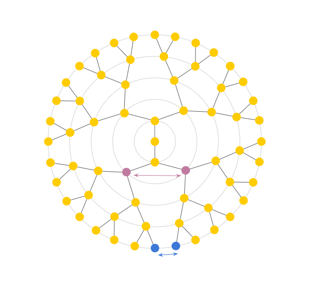
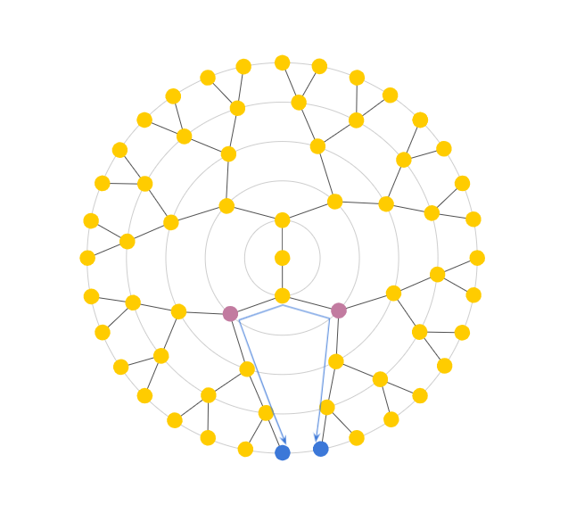
After an initial trial, where we struggled to get the program running on our systems, we discussed potential areas of research with Professor Campen and dived straight into the implementation of our ideas. The part of the algorithm that I worked on was concerned with the process of splitting given Bézier curves (for the purpose of creating a mesh), particularly how to choose the point of bisection, \(t\). During a later stage of the algorithm, the curves are enveloped by quadrilaterals (or two triangles with a curved edge). If two quads intersect, we must split one of the curves. The key idea here was that the quads could then potentially inform how the curves were to be split. Without going into too much technical detail, I essentially tried to implement different approaches to optimize the splitting process. The graph below shows a snippet of my results.

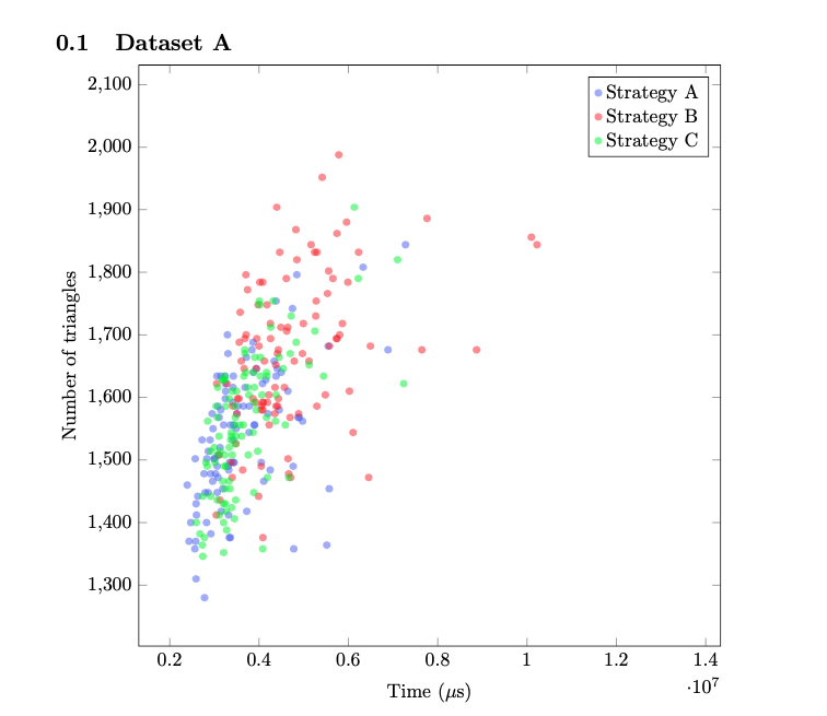
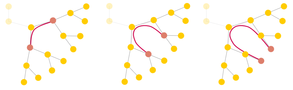
While Strategy A is the original algorithm implementation, Strategy B and C were possible improvements to it. For both of the latter strategies I used an area function to find the point where the resulting quads would have the approximately equal area. This equal distribution could point to an optimal solution. The difference between B and C has to do with how the value of \(t\) is iteratively changed as is shown below.

While I was only able to run the program on a sample size of 100 2D images, basic quantitative analysis pointed towards Strategy A and C as the more optimal choices. However, to get more conclusive results, the strategies need to be tested on more data. In addition to Strategy B and C, another direction for further consideration was to use the corners of the quad to find the projection of the closest corner to the curve.

As the week came to an end, I was sad to leave the project at this somewhat incomplete stage. During the week, I went from nervously reading my first research paper to testing potential improvements to it. It was an exciting week for me and I can’t wait to see what’s next!

By: Zeltzyn Montes and Sneha Sambandam

Many of the datasets we would like to perform machine learning on have an intrinsic hierarchical structure. This includes social networks, taxonomies, NLP sentence structure, and anything that can be represented as a tree. While the most common machine learning tools work in the Euclidean space, this space is not optimal for representing hierarchical data.

When representing hierarchical data in the 2D space, we have two main objectives: to preserve the hierarchical relationships between parent and child nodes; and to ensure distances between nodes are somewhat proportional to the number of links in between. However, when representing this structure in the 2D Euclidean space, we run into a few limitations.

Fig 1. A tree with branching factor of 2 drawn in the Euclidean space. (Courtesy of Alison Pouplin)

For example, let’s first draw a tree, with a branching factor of 2 (Fig 1). When our tree is very deep, placing nodes equidistantly causes us to run out of space rather quickly, like in our example above at only a depth of 5. The second problem we run into is with untrue distance relationships among nodes. To help visualize this phenomenon, refer to Fig 2a. Here, arc refers to the shortest path between two nodes.

—————————————— –Fig 2a.—————––––——– ——————————-–––—––– ——————–Fig 2b.
Euclidean vs desired measurement of distance between nodes.
(Courtesy of Alison Pouplin)

In theory, since the length of the arc between the purple nodes is less than that of the blue nodes, the purple nodes should result in the smaller distance. However, the Euclidean distance between the purple nodes is larger than the distance between the blue nodes. With the Euclidean 2D space, we observe that siblings in later generations end up closer and closer together, rendering Euclidean distance almost meaningless, as it only grows linearly with depth. Instead, we need a better distance measure: one that somehow travels “up” a tree before going back down as shown in Fig 2b and that is analogous to tree distance that grows exponentially as shown in Fig 3.

Fig 3. Desired measurement of distances between nodes. (Courtesy of Alison Pouplin)

A solution for this is to add an extra dimension (Fig 4). Now, the tree follows a smooth manifold: a hyperboloid. A hyperboloid is a manifold with a negative sectional curvature in the Minkowski space, drawn by rotating a parabola around its symmetrical axis. Note, the Minkowski space is similar to the Euclidean space except dimension 1 is treated differently, while other dimensions are treated similarly to the Euclidean space.

Fig 4. Adding a fourth dimension to hierarchical data. (Courtesy of Alison Pouplin)

Embedding the tree on a smooth manifold now allows us to compute geodesics (shortest distance between two points on a surface). We can also project the data onto a lower dimensional manifold, such as the Poincaré disk model. This model can be derived using a stereoscopic projection of the hyperboloid model onto the unit circle of the z = 0 plane (Fig 5).

Fig 5. Projecting hyperbolic geodesic to Poincaré disk. (Courtesy of Alison Pouplin)

The basic idea of this stereoscopic projection is:

Start with a point P on the hyperboloid we wish to map.
Extend P out to a focal point N = (0,0,−1) to form a line.
Project that line onto the z = 0 plane to find our point Q in the Poincaré model.

The Poincaré disk model is governed by the Möbius gyrovector space in the same way that Euclidean geometry is governed by the common vector space (i.e., we have different rules, properties and metrics that govern this space). While we won’t go into the specifics of what constitutes a gyrovector space, we shall detail the properties of the Poincaré disk that make it advantageous for representing hierarchical data.

Fig 6. A tree with branching factor of 2 drawn on the Poincaré disk. (Source)

In Fig 6, we can see a hierarchical tree with branching factor two embedding into a Poincaré disk. Distances between all points are actually equal because distances grow exponentially as you move toward the edge of the disk.

Some notable points of this model are the following:

The arcs never reach the circumference of the circle. This is analogous to the geodesic on the hyperboloid extending out to infinity, that is, as the arc approaches the circumference it’s approaching the “infinity” of the plane.
This means distances at the edge of the circle grow exponentially as you move toward the edge of the circle (compared to their Euclidean distances).
Each arc approaches the circumference at a 90 degree angle, this just works out as a result of the math of the hyperboloid and the projection. The straight line in this case is a point that passes through the “bottom” of the hyperboloid at (0,0,1).

With these properties we are able to represent data in a compact, visually pleasing and apt form using hyperbolic geometry. Current research explores how we can harness these properties in order to perform effective machine learning on hierarchical data.