By Zhecheng Wang, Zeltzyn Guadalupe Montes Rosales, and Olga Guțan
Note: This post describes work that has occurred between August 9 and August 20. The project will continue for a third week; more details to come.
I. Introduction
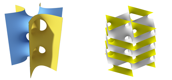
For the past two weeks we had the pleasure of working with Nicholas Sharp, Etienne Vouga, Josh Vekhter, and Erik Amezquita. We learned about a special type of minimal surfaces: triply-periodic minimal surfaces. Their name stems from their repeating pattern. Broadly speaking, a minimal surface minimizes its surface area. This is equivalent to having zero mean curvature. A triply-periodic minimal surface (TPMS) is a surface in \(\mathbb{R}^{3}\) that is invariant under a rank-3 lattice of translations.
Let’s talk about nonmanifold surfaces. “Manifold” is a geometry term that means: every local region of the surface looks like the plane (more formally — it is homeomorphic to a subset of Euclidean space). Non-manifold then allows for parts of the surface that do not look like the plane, such as T-junctions. Within the context of triangle meshes, a nonmanifold surface is a surface where more than 3 faces share an edge.
II. What We Did
First, we read and studied the 1993 paper by Pinkhall and Polthier that describes the algorithm for generating minimal surfaces. Our next goal was to generate minimal surfaces. Initially, we used pinned (Dirichlet) boundary conditions and regular manifold shapes. After ensuring that our code worked on manifold surfaces, we tested it on non-manifold input.
Additionally, our team members learned how to use Blender. It has been a very enjoyable process, and the work was deeply satisfying, because of the embedded mathematical ideas intertwined with the artistic components.
III. Reading the Pinkall Paper
“Computing Discrete Minimal Surfaces and Their Conjugates,” by Ulrich Pinkall and Konrad Polthier, is the classic paper on this subject; it introduces the iterative scheme we used to find minimal surfaces. Reading this paper was our first step in this project. The algorithm that finds a discrete locally area-minimizing surface is as follows:
- Take the initial surface \(M_0\) with boundary \(∂M_0\) as first approximation of M. Set i to 0.
- Compute the next surface \(M_i\) by solving the linear Dirichlet problem $$ \min_{M} \frac{1}{2}\int_{M_{i}}|\nabla (f:M_{i} \to M)|^{2}$$
- Set i to i+1 and continue with step 2.
The stopping condition is \(|\text{area}(M_i)-\text{area}(M_{i+1})|<\epsilon\). In our case, we used a maximum number of iterations, set by the user, as a stopping condition.
There are additional subtleties that must be considered (such as “what to do with degenerate triangles?”), but since we did not implement them — their discussion is beyond the scope of this post.
IV. Adding Periodic Boundary Conditions
This is, at its core, an optimization problem. To ensure that the optimization works, the boundary conditions have to be periodic instead of fixed in space. This is because we are enforcing a set of boundary conditions on periodic shapes — that is, tiling in a 3D space.
IV(a). Matching Vertices
First, we need to check every two pairs of vertices in the mesh. We are looking to see if they have identical coordinates in two dimensions, but are separated by exactly two units in the third dimension. When we find such pairs of vertices, we classify them to \(G_x\), \(G_y\), or \(G_z\). Note that we only store unique pairs.
IV(b). Laplacian Smoothness at the Boundary Vertices
Instead of using the discrete Laplacian, now we introduce a sparse matrix K to adjust our smoothness term based on the new boundary:
$$\min_{x}x^T(L^TK^TKL)x \text{ s.t. } x[b] = x_0[b].$$
Next, we construct the matrix K, which is a sparse square matrix of dimension #vertices by #vertices. To do so, we set \(K(i,i) = 1\), \(K(i,j) = 1\), and set the \(j\)th row entries to 0 for every pair of unique matched boundary vertices. For every interior vertex \(i\), we set \(K(i,i) = 1\).
IV(c). Aligning Boundary Vertices
Now we no longer want to pin boundary vertices to their original location in space. Instead, we want to allow our vertices to move, while the opposite sides of the boundary still match. To do that, we need to adjust the existing constraint term and to include additional linear constraints \(Ax=b\).
Therefore, we add two sets of linear constraints to our linear system:
- For any pair of boundary vertices distanced by 2 units in one direction, the new coordinates should differ by 2 units.
- For any pair of boundary vertices matched in the two other directions, the new coordinates should differ by 0.
We construct a selection matrix \(A\), which is a #pairs of boundary vertices in \(G\) by #vertices sparse matrix, to get the distance between any pair of boundary vertices. For every \(r\)th row, \(A(r,i)=1, A(r,j)=-1.\)$
Then we need to construct 3 \(b\) vectors, each of which is a sparse square matrix of the size [# of vector pairs of boundary vertices in G for a 3D coordinate (x,y,z)]. Based on whether at one given moment we are working with \(G_x\), \(G_y\), or \(G_z\), we enter \(2\) for those selected pairs, and \(0\) for the rest.
V. Correct Outcomes
Below, we can see the algorithm being correctly implemented. Each video represents a different mesh.
VI. Aesthetically Pleasing Bugs
Nothing is perfect, and coding in Matlab is no exception. We went through many iterations of our code before we got a functional version. Below are some examples of cool-looking bugs we encountered along the way, while testing the code on (what has become) one of our favorite shapes. Each video represents a different bug applied onto the same mesh.
VII. Conclusion and Future Work
Further work may include studying the physical properties of nonmanifold TPMS. It may also include additional basic structural simulations for physical properties, and establishing a comparison between the results for nonmanifold surfaces and the existing results for manifold surfaces.
Additional goals may be of computational or algebraic nature. For example, one can write scripts to generate many possible initial conditions, then use code to convert the surfaces with each of these conditions into minimal surfaces. An algebraic goal may be to enumerate all possible possibly-nonmanifold structures and perhaps categorize them based on their properties. This is, in fact, an open problem.
The possibilities are truly endless, and potential directions depend on the interests of the group of researchers undertaking this project further.
One reply on “Minimal Surfaces, But Periodic”
[…] week we worked on extending the results described here. We learned an array of new techniques and enhanced existing skills that we had developed the […]