topology – SGI 2021

Finding the Lower Bounds of the Hausdorff Distance

Author: Bryce Van Ross

Currently, we’re finishing the first half of the 2-week Robust computation of the Hausdorff distance between triangle meshes project. This research is lead by mentor Dr. Leonardo Sacht, TA Erik Amézquita, and in my immediate team, I work with fellow students Deniz Ozbay and Talant Talipov. The below is a brief summary of what’s happened so far:

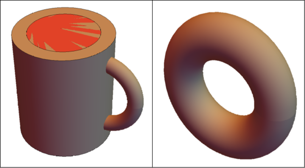
A mathematical visualization of the Hausdorff distance of two meshes

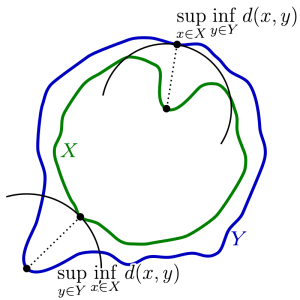
Source: https://en.wikipedia.org/wiki/Hausdorff_distance

Applications: Primarily computer vision, computer graphics, digital fabrication, 3D-printing, and modeling. For example, in computer vision, it is often desirable to identify a best-candidate target relative to some initial template. In reference to the set of points within the template, the Hausdorff distance can be computed for each potential target. The target with the minimum Hausdorff distance would qualify as being the best fit, ideally being a close approximation to the template object.

Motivation: Objects are geometrically complex. There are different ways to compare objects to each other via a range of geometry processing techniques and geometric properties. Distance is often a common metric of comparison. But what type of distance should we use, which distances are favorable, and why? These are important questions.

Pitfalls of using other types of distance for triangular meshes

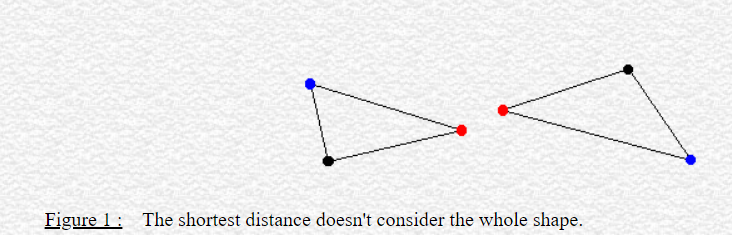
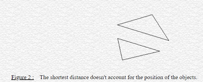
Source: http://cgm.cs.mcgill.ca/~godfried/teaching/cg-projects/98/normand/main.html

For our research, we focus on computing the Hausdorff distance \(h\). “Hausdorff” may seem familiar to you if you know topology. There, a (topological) space is considered Hausdorff if any two elements can be separated into disjoint (open) sets. The key idea here is the separation property with respect to points.

In geometry processing, this idea is extended (in some sense) to the separation of triangle meshes. The Hausdorff distance \(h\) is fundamentally a maximum distance among desirable distances between 2 meshes. These desirable distances are minimum distances of all possible vectors resulting from points taken from the first mesh to the second mesh. But why is \(h\) significant? If \(h\) converges to zero (the smallest possible distance), then this implies that our meshes, and therefore the objects themselves, are very similar. This, like most things in math, implies within some epsilon, representing marginal change such as a slight deformation, rotation, translation, compression, or stretch. If \(h\) is large, then this implies that the two objects are dissimilar. Intuitively, this is due to a lack of ideal correspondence from triangle to triangle. In short, \(h\) serves as a means of computing the similarity between digital objects in terms of maximally separating the meshes’ points according to their minimum distances.

Tasks: To compute \(h\), we find the maximizer, the point (in the first mesh) corresponding to the computation of \(h\). This point is found via an algorithmic process called the branch and bound technique. Sparing the details, the result of applying this technique will provide a (very small) region where the minimizer is claimed to exist, after a series of triangle subdivisions and deletions. There are different ways to implement this technique. Our collective goal this week was to achieve accurate \(h\) given any two meshes. Once this is ensured, Week 2 would focus on making our code more robust (efficient/fast). This work can be simplified into three primary tasks: encoding the lower bound and upper bound of possible values of \(h\), and the subdivision method. My work focused on the lower bound, for which the other two functions are dependent.

Accomplishments: By Day 2, we started with writing pseudocode for the lower bound, using only the vertices of the first mesh and computing their distances with respect to vertices of the second mesh. This was computed per face, and the minimum was found. Although this method was correct, it didn’t account for either the edge or interior cases of a given triangle. Looping through an edge would be immediately doable, but the interior case would be more challenging. Thankfully, Dr. Sacht had us search through gptoolbox for such functionality that would account for all three cases. Once finding this function, we were able to reduce my code to two lines! The irony is although this was valid, the referenced function was basically an empty shell. The function was actually calling a C++ function that would have to compiled and linked against other libraries and due to our time constraints we decided it was best to address this issue in a future time. Ultimately, we ended up having to write from scratch once more. In searching for similar point-triangle distance algorithms, we initially found an approach using normal vectors, which would offer projective power of the former mesh vertices relative to the latter mesh. The computations were erroneous and misrepresentative. Since then, our team has been using a combinatorial plane-vector approach to find the lower bounds per vertex.

Hopefully we’ll finish soon… we’re excited for the next steps!

There is a famous saying – A topologist is a person who can’t differentiate between a donut and a mug. At the first glance, this might sound very confusing… Donuts and mugs are two very different objects, so how can someone not be able to tell them apart? Well, to realize this joke, we first need to understand homeomorphisms. In this post, we will try to dig deeper into this concept, and then we will talk briefly about surface-to-surface mapping.

Before diving into the theoretical explanation, let us elucidate the matter with some interesting visualizations. Below is a picture of a basic 3D mug and a donut drawn in Wolfram Mathematica. (Disclaimer: The objects may not look very attractive, but let’s keep it this way for simplification)

Figure 1: A mug and a donut drawn in Wolfram Mathematica. (Source)

Now, if we look closely, we can change (or deform) the mug into a donut shape. The related code snippet and the deformation are shown below:

Figure 2: The corresponding Wolfram code that draws the mug and the donut in an interactive prompt. (Source)

Figure 3: The mug is being deformed into a donut. (Source)

We can also go back to our original mug shape from the donut shape. So, we can say that this change is invertible and bijective:

Figure 4: The mug and the donut are being deformed into each other. (Source)

So far, we have seen that we can deform a mug into a donut and vice versa. In other words, we can say there is a map between these two shapes. In mathematical definition, this phenomenon is known as homeomorphism. To be more concise, two shapes are called to be homeomorphic when there is a map between them that is continuous, invertible, and bijective.

Now that we have a basic understanding of homeomorphism, let’s dive deeper into this matter. In the donut and mug example above, we manually designed a deformation function that mapped between these objects. This map will not always work for every other shape we encounter. Moreover, it will be very tedious to manually find every map between all possible pairs of shapes. So, we need to find a generic solution that will work for a larger class of shapes. In geometric terms, this task is commonly referred to as “Surface-to-Surface Mapping”. This task is especially useful for a wide range of geometric applications, such as shape correspondence, texture transfer, layout transfer, and abstract layout embedding.

In the SGP 2021 Graduate School, there was a session titled “Maps Between Surfaces” by M. Campen and P. Schmidt, where the authors described different methods of surface-to-surface mapping in detail. I am deeply intrigued by their talk, and much of the later part of this post has been inspired by their talk.

To understand the concept of surface-to-surface mapping, we need to understand plane-to-plane mapping and surface-to-plane mapping first. In simple terms, plane-to-plane mapping is a homeomorphic map that takes a 2D plane to a different 2D plane. Similarly, surface-to-plane mapping is a homeomorphic map that takes a surface (represented as a triangular mesh) to a 2D plane. But, this might not always be possible for non-disk surfaces. For example, no matter how much we try, a homeomorphic map can’t be found between a 3D sphere and a plane. In such cases, we will use a cut graph to simplify our 3D surface representation.

We are now ready to look at different representation techniques of surface-to-surface mapping:

Deduction to surface-to-plane mapping (for smooth surface): We can deduce the problem to a simpler surface-to-plane mapping problem. That is, surface A would be mapped to a plane C, and C would be mapped to the other surface, B.
Vertex to ambient map: In this map, we store the corresponding 3D coordinate of each vertex of surface A.
Vertex to surface map: Instead of directly storing the 3D coordinate, we store the corresponding triangle ID and relative position on surface B for each vertex of A.
Vertex to vertex map: For every vertex of surface A, we store a vertex of surface B.
Functional map: In this setting, we represent the mapping using low-frequency functions (for example, from a Laplacian eigenbasis of the mesh).

However, each of these settings has some disadvantages. The common problem is that all of these maps are only storing information for vertices of A, but not other points on A (such as the points that lie on the edges). Hence, it might be difficult to find the inverse map from surface B to surface A. In other words, these maps are not bijective. For defining perfect homeomorphisms, we can take inspiration from Gauss-Bonnet Theorem. Using this theorem, we can map shapes with 0, 1 and greater than one genus to sphere, plane and hyperbolic plane using Poincare model, Beltrami-Klein model, and hyperboloid model, respectively, so that bijectivity is ensured.

Apart from homeomorphism, a surface-to-surface map must also abide by some other constraints: it has to ensure a low distortion rate, abide by semantic and topological constraints. These constraints can be satisfied by following a two-step approach, consisting of map initialization and map optimization. The authors also described in detail how this approach works. As this is out of the scope of this post, we will not look deeper into those techniques. Interested readers are encouraged to watch their full session here: https://youtu.be/jMWJ79EpyfQ.