Foqia – SGI 2021

Isogeometric analysis (IGA) is an analysis technique that combines computer aided design (CAD) with traditional finite element analysis (FEA). It uses the same spline basis functions to construct the geometry and the solution space, which is beneficial as traditional FEA requires geometric approximation that can lead to inaccuracies [1].

For our week 3 project, my group and I used IGA simulation software that has been developed for modelling material transport in neurons. The software solves Navier-Stokes equations to obtain the velocity field and models the transport process by reaction-diffusion-transport equations. For our purposes, we used the solver to simulate material transport in complex neurons and heat transfer processes in various geometries including a simple block model and a rod model [2].

Our project was split into two main parts: geometric modeling and analysis. For geometric modelling, we used two open source software packages (HexGen and Hex2Spline [3]) for the construction of geometries, and we then used the aforementioned IGA software for simulation purposes. I was in charge of using the IGA software to run the simulations and visualizing the results with Paraview (a visualization application).

In this post, I’ll demonstrate our results using the simple model the team created and also share some of the results I got using the IGA software on some additional models.

Here is the example model we used:

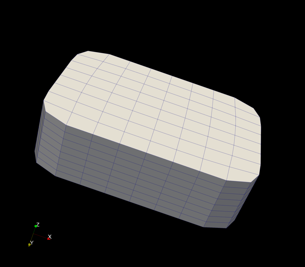
After the geometric modeling stage, I received 3 input files that contained the control mesh, an initial velocity field and the simulation parameters (particle concentrations, diffusion coefficient, velocities of material, etc.). These files were used as input for the IGA solver [2], which consists of four stages: spline construction, mesh partition for parallel computing, solving Navier-Stokes equations, and final transport simulation.

Due to the high computational needs of the last two stages, we set up the simulation environment at the Pittsburgh Supercomputer Center (PSC). We ran the simulation by connecting to the remote supercomputer via an ssh client. Finally, after getting the results, I was able to visualize them using Paraview.

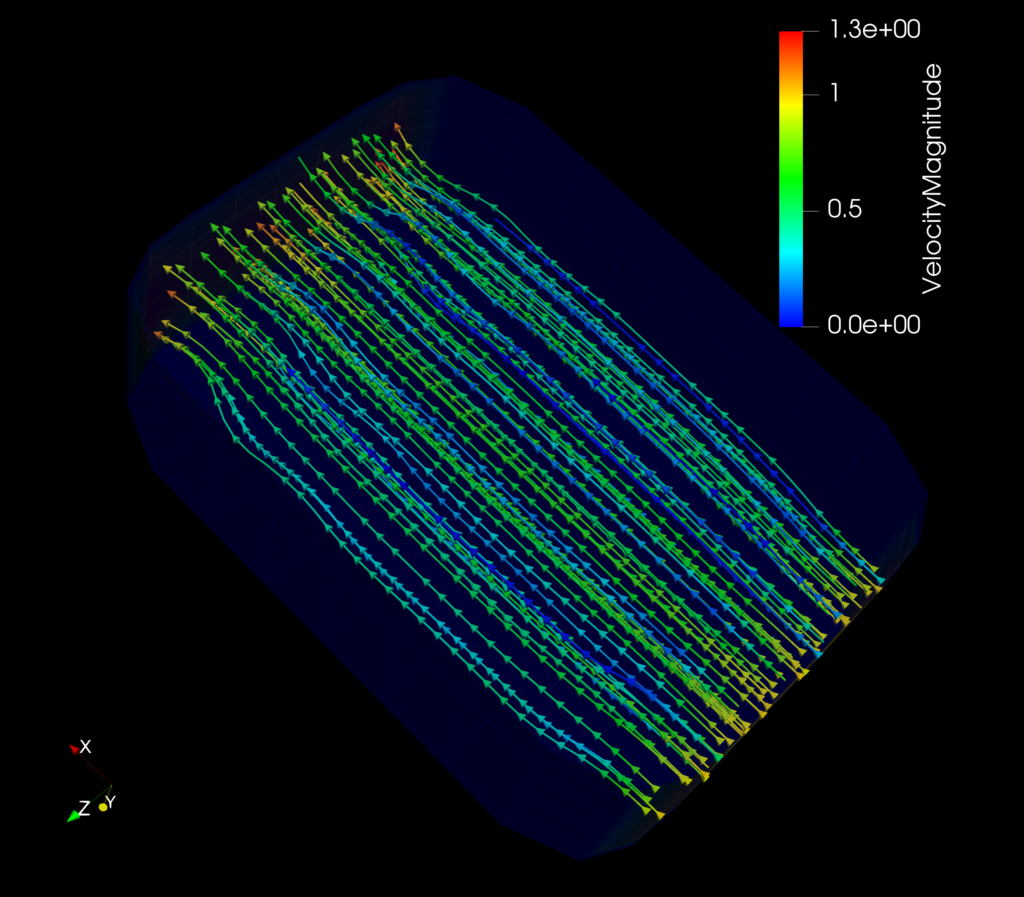
In the above example, the color bar shows the transport velocity magnitude. I also added streamlines that show the direction of flow.

Here is an animation of our results that depicts the movement of the particles:

I also ran the solver on a rod model (that Angran Li, our mentor, provided):

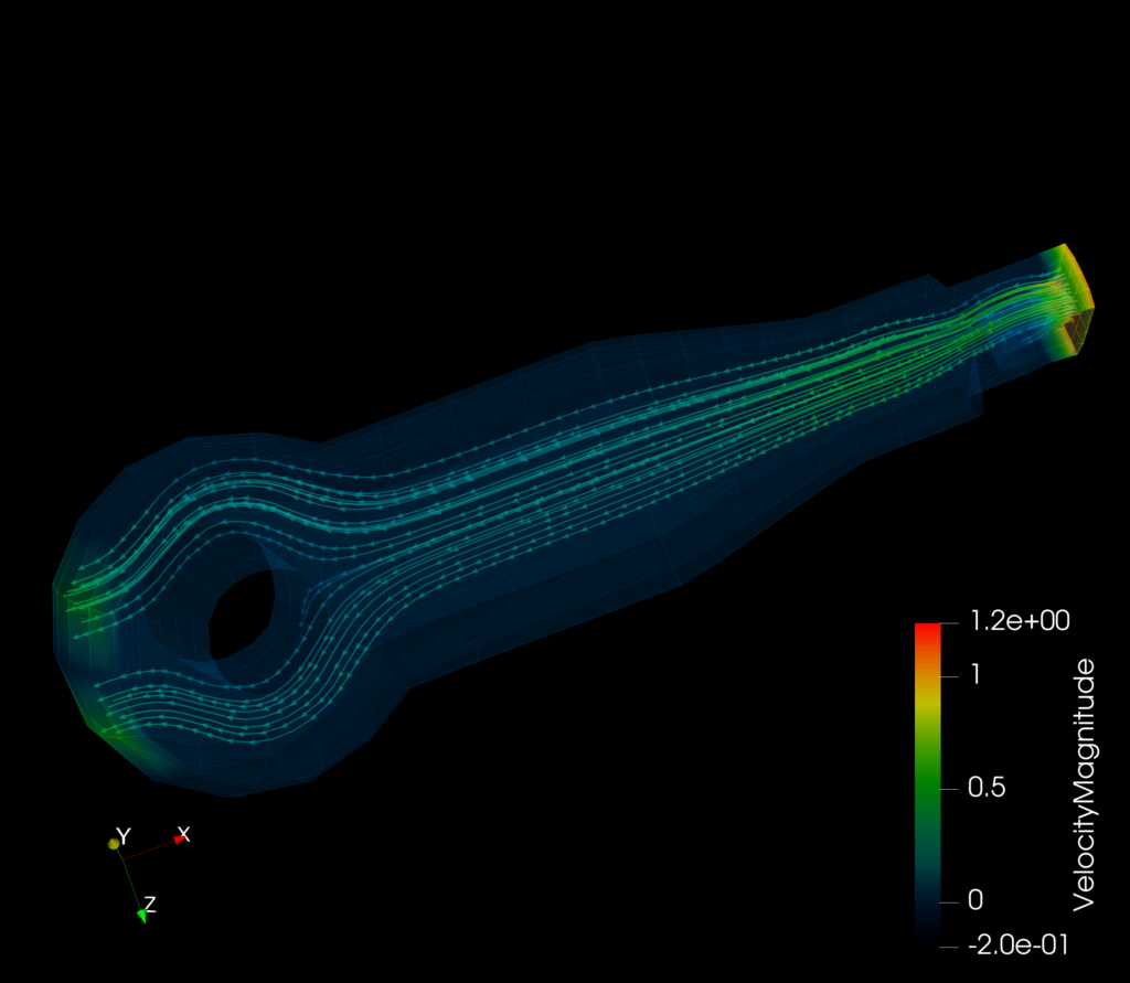
The model shows the flow of heat through the rod as it is input from the right end of the model. Again, the colorbar represents the magnitude of the velocity of particles at that point.

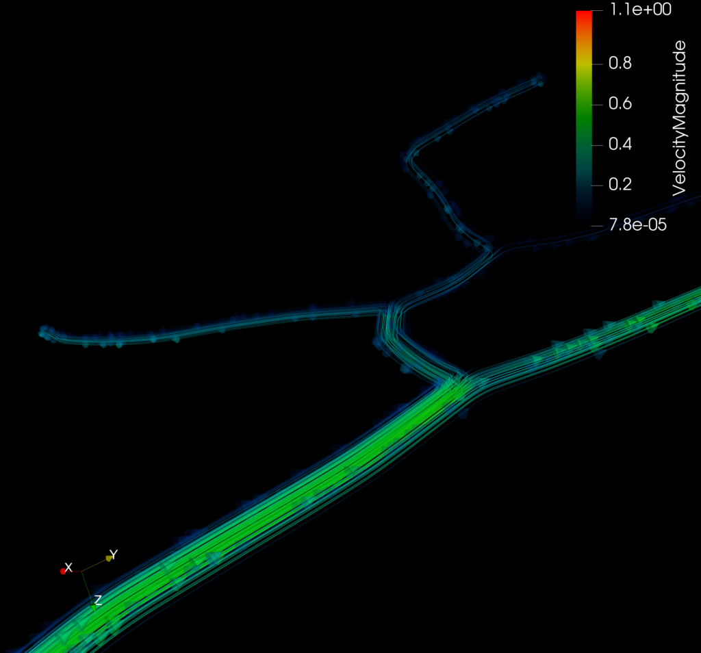
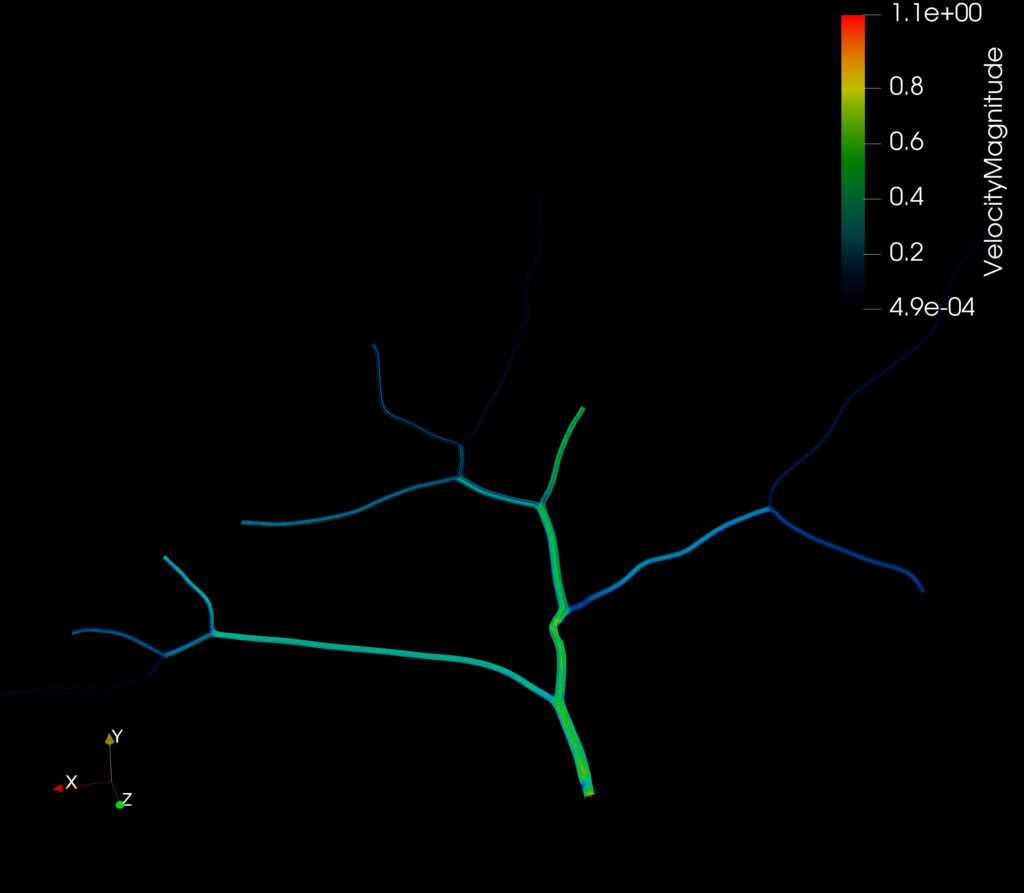
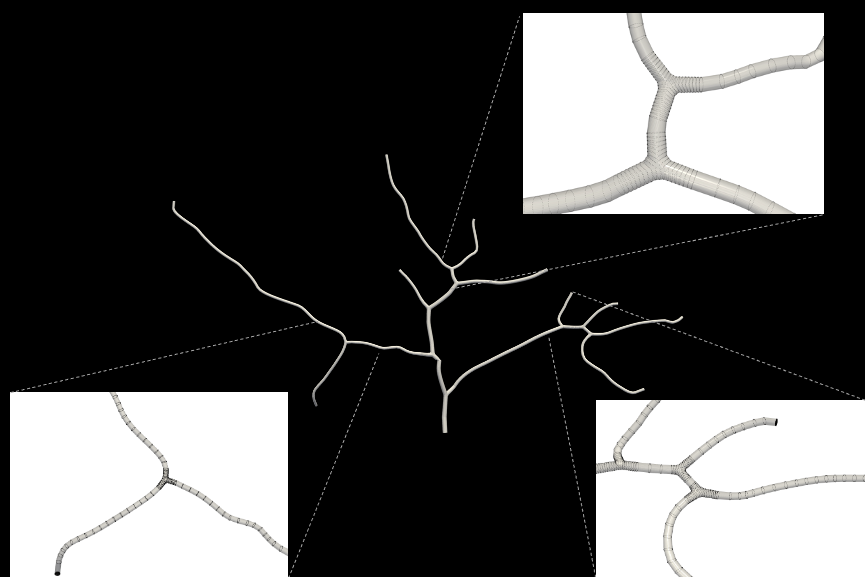
Finally, I also ran the IGA solver on a neuron model (found on NeuroMorpho.org and edited with the help of Angran).

The geometry of the neuron (visualised using Paraview)

Images show results we got by running the IGA solver on the neuron geometry

The transport of material through the neuron over time

From using the remote computer to editing the neurons for our analysis, I learned a ton of new techniques during the week. I enjoyed learning about the IGA solver and its applications ranging from neuroscience to engineering. I’d like to end this post by thanking Angran his support and for bearing with me through my 1000 questions—it was a pleasure learning with you! 🙂

References:

[1] T. J. Hughes, J. A. Cottrell, Y. Bazilevs. Isogeometric analysis: CAD, finite elements, NURBS, exact geometry and mesh refinement. Computer Methods in Applied Mechanics and Engineering, 194(39-41), 4135-4195, 2005.

[2] A. Li, X. Chai, G. Yang, Y. J. Zhang. An Isogeometric Analysis Computational Platform for Material Transport Simulations in Complex Neurite Networks. Molecular & Cellular Biomechanics, 16(2):123-140, 2019. GitHub link: https://github.com/CMU-CBML/NeuronTransportIGA

[3] Y. Yu, X. Wei, A. Li, J. G. Liu, J. He, Y. J. Zhang. HexGen and Hex2Spline: Polycube-Based Hexahedral Mesh Generation and Unstructured Spline Construction for Isogeometric Analysis Framework in LS-DYNA. Springer INdAM Serie: Proceedings of INdAM Workshop “Geometric Challenges in Isogeometric Analysis”. Rome, Italy. Jan 27-31, 2020. GitHub link: https://github.com/CMU-CBML/HexGen_Hex2Spline

As the whirlpool of the first week of SGI came to an end, I felt that I’d learnt so much and perhaps not enough at the same time. I couldn’t help but wonder: Did I know enough about geometry processing (…or was it just the Laplacian) to actually start doing research the very next week? Nevertheless, I tried to overcome the imposter syndrome and signed up to do a research project.

I joined Professor Marcel Campen’s project on “Improved 2-D Higher Order Meshing” for Week 2. The project focused particularly on higher order triangle meshes, which are characterized by their curved (rather than straight) edges. We studied a previously presented algorithm for the generation of these meshes in 2D, with the goal of improving or generalizing it.

After an initial trial, where we struggled to get the program running on our systems, we discussed potential areas of research with Professor Campen and dived straight into the implementation of our ideas. The part of the algorithm that I worked on was concerned with the process of splitting given Bézier curves (for the purpose of creating a mesh), particularly how to choose the point of bisection, \(t\). During a later stage of the algorithm, the curves are enveloped by quadrilaterals (or two triangles with a curved edge). If two quads intersect, we must split one of the curves. The key idea here was that the quads could then potentially inform how the curves were to be split. Without going into too much technical detail, I essentially tried to implement different approaches to optimize the splitting process. The graph below shows a snippet of my results.

While Strategy A is the original algorithm implementation, Strategy B and C were possible improvements to it. For both of the latter strategies I used an area function to find the point where the resulting quads would have the approximately equal area. This equal distribution could point to an optimal solution. The difference between B and C has to do with how the value of \(t\) is iteratively changed as is shown below.

While I was only able to run the program on a sample size of 100 2D images, basic quantitative analysis pointed towards Strategy A and C as the more optimal choices. However, to get more conclusive results, the strategies need to be tested on more data. In addition to Strategy B and C, another direction for further consideration was to use the corners of the quad to find the projection of the closest corner to the curve.

As the week came to an end, I was sad to leave the project at this somewhat incomplete stage. During the week, I went from nervously reading my first research paper to testing potential improvements to it. It was an exciting week for me and I can’t wait to see what’s next!