Natasha – SGI 2021

By: Judy Chiang, Natasha Diederen, Erick Jimenez Berumen

Project mentor: Christian Hafner

Architects often want to create visually striking structures that involve curved materials. The conventional way to do this is to pre-bend materials to form the shape of the desired curve. However, this generates large manufacturing and transportation costs. A proposed alternative to industrial bending is to elastically bend flat beams, where the desired curve is encoded into the stiffness profile of the beam. Wider sections of the beam will have a greater stiffness and bend less than narrower sections of the beam. Hence, it is possible to design an algorithm that enables a designer or architect to plan curved structures that can be assembled by bending flat beams. This is a topic currently being explored by Bernd Bickel and his student Christian Hafner (our project mentor).

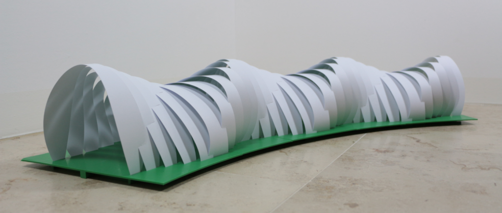
A model created using the concept of active bending (source)

For the flat beam to remain bent as the desired curve, we must ensure that the beam assumes this form at its equilibrium point. In Lagrangian mechanics, this occurs when energy is minimised, since this implies that there is no other configuration of the system which would result in lower overall energy and thus be optimal instead. Two different questions arise from this formulation. First, given the stiffness profile \(K\), what deformed shapes \(\gamma\) can be generated? Second, given a curve \(\gamma\), what stiffness profiles \(K\) can be generated? In answering the first problem we will find the curve that will result from bending a beam with a given width profile. However, we are more interested in finding the stiffness profile of a beam which will result in a curved shape \(\gamma\) of our choice. Hence, we wish to solve the second problem.

Below, we will give a full formulation of our main problem, and discuss how we transformed this into MATLAB code and created a user interface. We will conclude by discussing a more generalised case involving joint curves.

Problem formulation

To recap, the problem we want to solve is, given a curve \(\gamma \), what stiffness profiles \(K\) can be generated? For each point \(s\) on our curve \(\gamma: (0,\ell) \to \mathbb{R}^2\), we have values for the position \(\gamma(s)\), turning angle \(\alpha(s)\), and signed curvature \(\alpha'(s)\). In addition, we define the energy of the beam system to be \[W[\alpha] := \int_0^\ell K(s)\alpha'(s)^2 ds,\] where \(K(s)\) is the stiffness at point \(s\). At the equilibrium state of the system, \(W[\alpha]\) will take a minimum value. Intuitively, this implies that, in general, regions of larger curvature will have a lower stiffness. However, it is not true that two different points of equal curvature will have equal stiffness, since there are other factors at play.

Now, before finding the \(K\) that minimises \(W[\alpha]\), we must set additional constraints \[\alpha(0) = \alpha_0, \quad \alpha(\ell) = \alpha_\ell\] and \[\gamma(0) = \gamma_0, \quad \gamma(\ell) = \gamma_\ell.\] In words, we are fixing the turning angles (tangents) and positions of the two boundary points. These constraints are necessary, since they dictate the position in space where the curve begins and ends, as well as the initial and final directions the curve moves in.

We have now formulated a problem that can be solved using variational calculus. Without going into detail, we find that stationary points of this function are given by the equation \[K \kappa = a + \langle b, \gamma \rangle,\] where \(\kappa\) is the signed curvature (previously \(\alpha’\)), and \(a \in \mathbb{R}\) and \(b \in \mathbb{R}^2\) are constants to be found. However, a stiffness profile cannot be generated for all curves \(\gamma\). More specifically, it was shown by Bernd Bickel and Christian Hafner that a solution exists if and only if there exists a line \(L\) that intersects \(\gamma\) exactly at its inflections. With this information in hand, we can begin to create a linear program that computes the stiffness function \(K\).

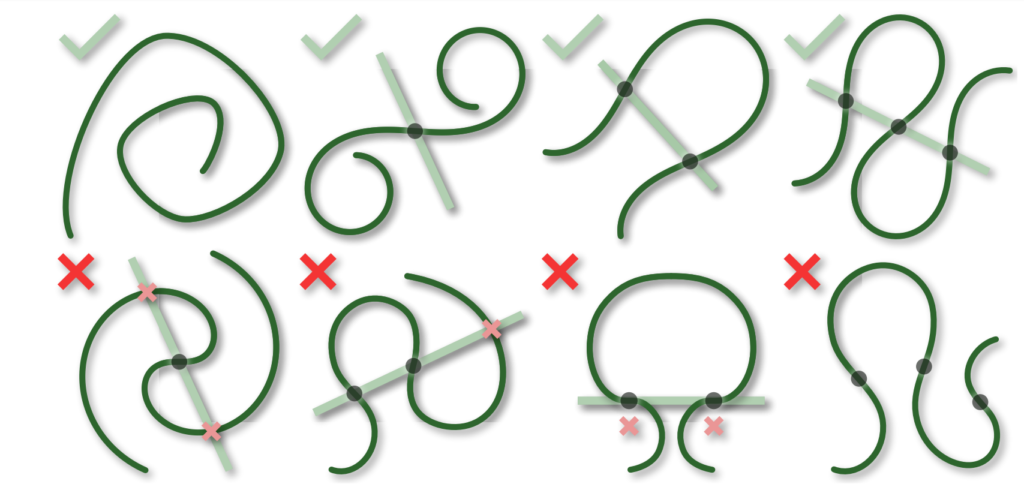
The top four curves can be created using active bending, but the bottom four cannot (source)

Creating a linear programme

In order to find the stiffness \(K\), we need to solve for the constants \(a\) and \(b\) in the equation \( K \kappa = a + \langle b, \gamma \rangle \), which can be discretised to \[ K(s_i) = \frac{a + \langle b, \gamma(s_i) \rangle }{\kappa(s_i)}.\] It is possible that there is more than one solution to \(K\), so we want some way to determine the “best” stiffness profile. If we think back to our original problem, we want to ensure that our beam is maximally uniform, since this is good for structural integrity. Hence, we solve for \(a\) and \(b\) in the above inequality in such a way that the ratio between maximum and minimum stiffness is minimised. To do this we set the minimum stiffness to an arbitrary value, for example 1, and then constrain \(K\) between 1 and \(M = \text{min}_i K_i\), thus obtaining the inequality \[1 \leq \frac{a + \langle b, \gamma(s_i) \rangle }{\kappa(s_i)} \leq M.\] This can be solved using MATLAB’s linprog function (read the documentation here). In this case, the variables we want to solve for are \(a \in \mathbb{R}\), \(b \in \mathbb{R}^2\), and \(M\) (a scalar we want to minimise). So, using the linprog documentation \(x\) is the vector \((a,b_1,b_2,M)\) and \(f\) is the vector \((0,0,0,1)\), since \(M\) is the only variable we want to minimise. Since linprog only deals with inequalities of the form \(A \cdot x \leq b\), we can split the above inequality into two and write it in terms of the elements of \(x\), like so: \[-\Bigg(\frac{1}{\kappa(s_i)}a + \frac{\gamma_x(s{i})}{\kappa(s_i)}b_1 + \frac{\gamma_y(s_{i})}{\kappa(s_i)}b_2 + 0\Bigg) \leq -1,\] \[\frac{1}{\kappa(s_i)}a + \frac{\gamma_x(s_{i})}{\kappa(s_i)}b_1 + \frac{\gamma_y(s_{i})}{\kappa(s_i)}b_2 -M \leq 0.\]
These two equations are of a form that can be easily written into linprog to obtain the values of \(a\), \(b\) and \(M\) and hence \(K\).

User Interface

Once we solved the linear program outlined above, we created a user interface in MATLAB that would allow users to draw and edit a spline curve and see the corresponding elastic strip created in real time. Custom splines can be imported as a .txt file in the following format

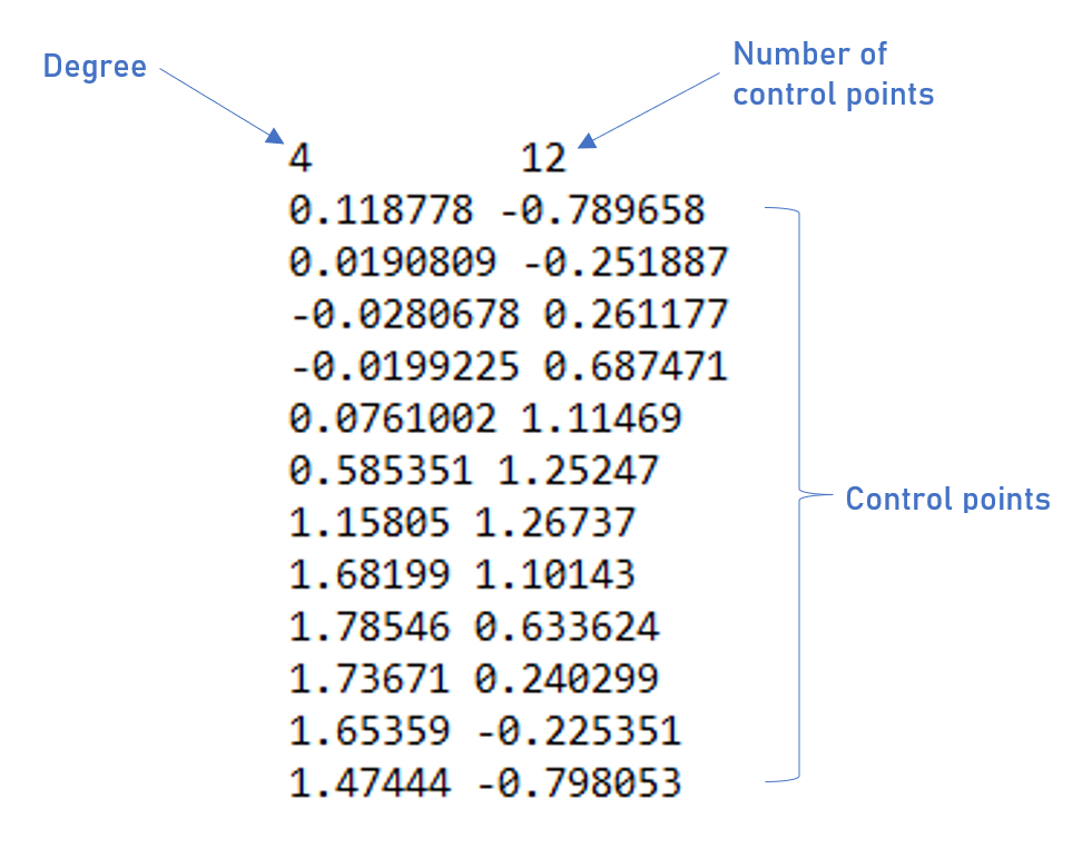
or alternatively, the file that is already in the folder can be used. Users can then run the user interface and edit the spline in real time. To add points, simply shift-click, and a new point will be added at the midpoint between the selected point and the next point. The user can right-click to delete a point, and left-click and drag to move points around. If there are zero or one control points remaining, then the user can add a new point where their mouse cursor is by shift-clicking. The number of control points must be greater than or equal to the degree plus one for the spline to be formed.
There are certain cases in which the linear program cannot be solved. In these cases the elastic strip is not plotted, and the user must move the control points around until it is possible to create a strip.

Demonstration of the user interface

Here is the link to the GitHub repository, for those who want to try the user interface out.

Joints Between Two or More Strips

The current version of our code is able to generate elastic strips for any (feasible) spline curve generated by the user. However, an as of yet unsolved problem is the feasibility condition for a pair of elastic strips with joints. Solving this problem would allow us compute a pair of stiffness functions \(K_1\) and \(K_2\) that yield elastic strips that can be connected via slots at the fixed joint locations. With a bit of maths we were able to derive the equilibrium equations that would produce such stiffness functions. Suppose the two spline curves are given by \(\gamma_{1}: [0,\ell_{1}] \to \mathbb{R}^2\) and \(\gamma_{2}: [0,\ell_{2}] \to \mathbb{R}^2\) and that they intersect at exactly one point such that \(\gamma_{1}(t_a) = \gamma_{2}(t_b)\). Then we must solve the following two equations: \[ K_{1}(t) \kappa_{1}(t) = \left \{ \begin{array}{ll} a_1 + \langle b_1, \gamma_{1}(t) \rangle + \langle c, \gamma_{1}(t) \rangle & 0 \leq t \leq t_a \\ a_1 + \langle b_1, \gamma_{1}(t) \rangle + \langle c, \gamma_{1}(t_a) \rangle & t_a < t \leq \ell_{1} \end{array}\right. \] \[ K_{2}(t) \kappa_{2}(t) = \left \{ \begin{array}{ll} a_2 + \langle b_2, \gamma_{2}(t) \rangle – \langle c, \gamma_{2}(t) \rangle & 0 \leq t \leq t_b \\ _2 + \langle b_2, \gamma_{2}(t) \rangle – \langle c, \gamma_{2}(t_b) \rangle & t_b < t \leq \ell_{2} \end{array}\right. \]

Similar to the one-spline case, these can be translated into a linear program problem which can be solved. Due to the time constraint of this project, we were not able to implement this into our code and build an associated user interface for creating multiple splines. Furthermore, above we have only discussed the situation with two curves and one joint. Adding more joints would increase the number of unknowns and add more sections to the above piece-wise-defined functions. Lastly, we are still lacking a geometric interpretation for the above equations. All of these issues regarding the extension to two or more spline curves would serve as great inspiration for further research!

An exploration of computational fluid dynamics

By: Natasha Diederen, Joana Portmann, Lucas Valença

These past two weeks, we have been working with Paul Kry to extend Jos Stam’s work on stable, incompressible fluid flow simulation. Stam’s paper Flows on Surfaces of Arbitrary Topology implements his stable fluid algorithm over patches of Catmull-Clark subdivision surfaces. These surfaces are ideal since they are smooth, can have arbitrary topologies, and have a quad patch parameterisation. However, Catmull-Clark subdivision surfaces are a quite specific class of surface, so we wanted to explore whether a similar algorithm could be implemented on triangle meshes to avoid the subdivision requirement.

Understanding basics of fluid simulation algorithms

We spent the first week of our project coming to terms with the different components of fluid flow simulation, which is based on solving the incompressible Navier-Stokes equation for velocities (1) and a similar advection-diffusion equation for densities (2) \[ \frac{\partial \mathbf{u}}{\partial t} = \mathbf{P} { -(\mathbf{u} \cdot \nabla)\mathbf{u} + \nu \nabla^2 \mathbf{u} + \mathbf{f} }, \quad (1)\] \[\frac{\partial \rho}{\partial t} = -(\mathbf{u} \cdot \nabla)\rho + \kappa \nabla^2 \rho + S, \quad (2)\] where \( \mathbf{u}\) is the velocity vector, \(t\) is time, \(\mathbf{P}\) is the projection operator, \( \nu\) is the viscosity coefficient, \(\mathbf{f}\) are external sources, \( \rho\) is the density scalar, \( \kappa\) is the diffusion coefficient, and \( S \) are the external sources. In the above equations, the Laplacian (often denoted \( \Delta\)) is written as \( \nabla^2\), as is usually done in works from the fluids community.

In his paper, Stam uses a splitting technique to deal with each term on its own. The algorithm carries out the following steps twice: first for the velocities and then for the densities (with no “project” step required for the latter). \[ \mathbf{u_0} {\underset{\overbrace{\text{add force}}^\text{ }}{\Rightarrow}} \mathbf{u_1} {\underset{\overbrace{\text{diffuse}}^\text{ }}{\Rightarrow}} \mathbf{u_2} {\underset{\overbrace{\text{advect}}^\text{ }}{\Rightarrow}} \mathbf{u_3} {\underset{\overbrace{\text{project}}^\text{ }}{\Rightarrow}} \mathbf{u_4} \]

Source: Flows on Surfaces of Arbitrary Topology

We start by adding any forces or sources we require. In the vector case, we can add acceleration forces such as gravity (which changes the velocities) or directly add velocity sources with a fixed location, direction, and intensity. In the scalar case, we add density sources that directly affect other quantities.

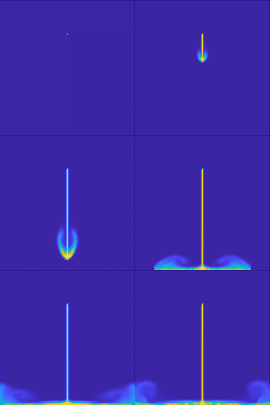
Single density source pouring down with gravity over an initially zero velocity field

Densities and velocities are moved from a high to low concentration in the diffusion step, then moved along the vector field in the advection step. The final projection step ensures incompressible flow (i.e., that mass is conserved), using a Helmholtz-Hodge decomposition to force a divergence-free vector field. We will not go into much more detail on Stam’s original Stable Fluids solver. Dan Piponi’s Papers We Love presentation gives a very comprehensive introduction for those interested in learning more.

To better understand the square grid fluids solver, we implemented a MATLAB version of the C algorithm described in Stam’s paper Real-Time Fluid Dynamics for Games. In terms of implementation, since we were coding in MATLAB, we did not use the Gauss-Seidel algorithm (like Stam did) to solve the minimisation problems. Instead, we solved our own quadratic formulations directly. Although some of our methods differed from the original, the overall structure of the code remained the same.

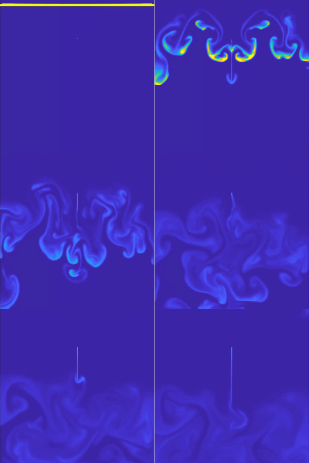
Full simulation results over a square grid can be seen below.

Generalising to triangle meshes

After a week, we understood the stable fluid algorithm well enough to extend it to triangle meshes. Stam’s paper for triangle meshes adapted the algorithm above from square grids to patches of a Catmull-Clark subdivided mesh, with the simulation boundary conditions at the edges of the parametric surfaces. We, on the other hand, wanted a method that would work over any triangular mesh, as long as such mesh, as a whole, is manifold without boundary. Moreover, we wished to do so by working directly with the triangles in the mesh without relying on subdivision surfaces for parameterisation. The main difference between our method and Stam’s was the need to deal with the varying angles between adjacent faces and their effect on advection, diffusion, and overall interpolation. In addition, since we’re working with manifolds without boundaries, we did not need to deal with boundary conditions (like in our 2D implementation). Furthermore, we had to choose between storing both vector and scalar quantities at the barycentre of each face or at each vertex. For simplicity, we chose the former.

What follows is a detailed explanation of how we implemented the three main steps of the fluid system: diffusion, advection and projection.

Diffusion

To diffuse quantities, we solved the equation\[ \dot{\mathbf{u}} = \nu \nabla^2 \mathbf{u},\] which can be discretised using the backwards Euler method for stability as follows \[ (\mathbf{I}-\Delta t \nu \nabla^2)\mathbf{u_2} = \mathbf{u_1}.\] Here, \( \mathbf{I} \) is the identity matrix and \( \mathbf{u_1}, \ \mathbf{u_2} \) are the respective original and final quantities for that iteration step, and can be either densities or vectors.

Surprisingly, this was far easier to solve for a triangle mesh than a grid due to the lack of boundary constraints. However, we needed to create our own Laplacian operators. They were used to deal with the transfer of density and velocity information from the barycentre of the current triangle to its three adjacent triangles. The first Laplacian we created was a linear operator that worked on vectors. For each face, before combining that face’s and its neighbours’ vectors with Laplacian weighting, it locally rotated the vectors lying on each of the face’s neighbouring faces. This way, the adjacent faces lay on the same plane as the central one. The rotated vectors were further weighted according to edge length (instead of area weighting) since we thought this would best represent flux across the boundary. The other Laplacian was a similar operator, but it worked on scalars instead of vectors. Thus, it involved weighting but not rotating the values at the barycentres (since they were scalars).

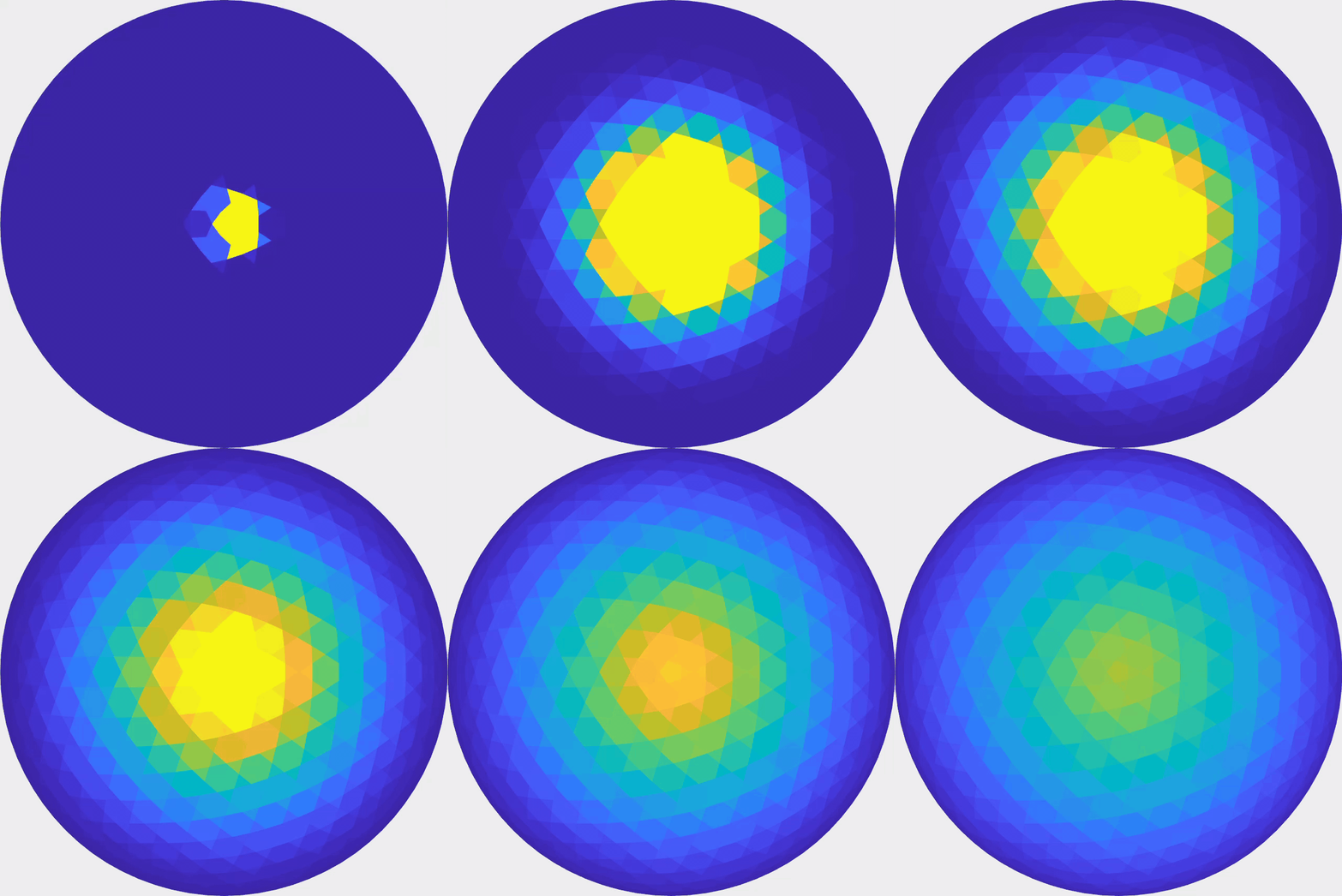
Diffusion of scalars over a flattened icosahedron

Advection

Advection was the most involved part of our code. To ensure the system’s stability, we implemented a linear backtrace method akin to the one in Stam’s Stable Fluids paper. Our approach considered densities and velocities as quantities currently stored at barycentres. It first looked at the current velocity at a chosen face then walked along the geodesic in the opposite direction (i.e., back in time). This allowed us to work out which location on the mesh we started at so that we would arrive at the current face one time-step later. This is analogous to Stam’s 2D walking over a square grid, interpolating quantities at the grid centres, but with a caveat. To walk the geodesics, we first had to use barycentric coordinates to work out the intersections with edges. Each time we crossed an edge, we rotated the walk direction vector from the current face to the next, making it as if we were walking along a plane. At the end of the geodesic, we obtain the previous position for the quantity on our current position. We then carried out a linear interpolation using barycentric coordinates and pre-interpolated vertex data. The result determined the previous value for the quantity in question. This quantity was then transported back to the current position. Vector quantities were also projected back onto the face plane at the end to account for any numerical inaccuracies that may have occurred.

Our advection code initially involved walking a geodesic for each mesh face, which is not computationally efficient in MATLAB. Thus, it accounted for the majority of the runtime of our code. The function was then mexed to C++, and the application now runs in real-time for moderately-sized meshes.

Projection

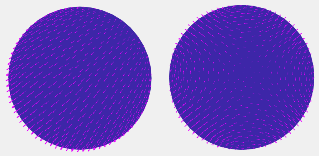
So far, we have not guaranteed that diffusion and advection will result in incompressible flow. That is, the amount of fluid flowing into a point is the same as the amount of fluid flowing out. Hence, we need some way of creating such a field. According to the Helmholtz-Hodge decomposition, any vector field can be decomposed into curl-free and divergence-free fields, \[ \mathbf{w} = \mathbf{u} + \nabla q, \] where \( \mathbf{w}\) is the velocity field, \( \mathbf{u} \) is the divergence-free component, and \( \nabla q\) is the curl-free component.

A solution (for \(q\)) is implicitly found by solving a Poisson equation of the form \[ \nabla \cdot \mathbf{w} = \nabla^2 q\] where we used the cotangent Laplacian in gptoolbox for \(\nabla^2 q\). Subtracting the solution from the original vector field gives us the projection operator \( \mathbf{P}\) to find the divergence free component \( \mathbf{u} \) \[\mathbf{u} = \mathbf{Pw}=\mathbf{w}-\nabla q. \]

A uniform vector field before (left) and after (right) projection

This method works really nicely for our choice of having vector quantities stored at the faces. The pressures we get will be at the vertices. The gradients of those pressures are naturally computed at faces to alter the velocities to give an incompressible field. The only challenge is that the Laplacian is not full rank, so we need to regularise it by a small amount.

Future work

We would like to implement an alternative advection method, possibly more complicated. This method would involve interpolating vertex data and walking along mesh edges, rather than storing all our data in faces and walking geodesics crossing edges. This could possibly avoid extra blurring, which might be introduced by our current implementation. This occurs because we must first interpolate the data at the neighbouring barycenters to the vertices. This data is then used to do a second interpolation back to the barycentric coordinate the geodesic ends at.

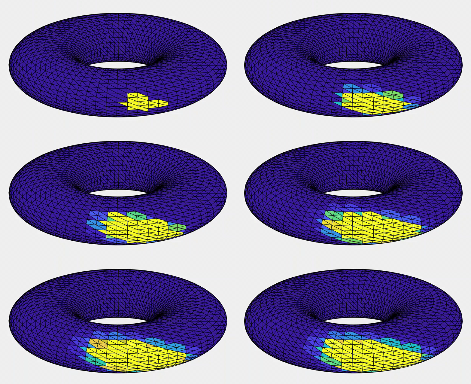
For diffusion, although our method worked, there were a few things that could be improved upon. Mainly, diffusion did not look isotropic in cases with very thin triangles, which could be improved by an alternative to our current weighting of the Laplacian operator. Alternatively, we could use a more standard Laplacian operator if we stored quantities at the vertices instead of barycenters. This would result in more uniform diffusion at the expense of a more complicated advection algorithm.

Example of non-isotropic diffusion over a flattened torus

Conclusion

Final results

We would like to give a thousand thanks to Paul Kry for his mentorship. As a first foray into fluid simulations, this started as a very daunting project for us. Still, Paul smoothly led us through it by having dozens of very patient hours of Zoom calls, where we learned a lot about maths and coding (and biking in the rain). His enthusiasm for this project was infectious and is what enabled us to get everything working in such a short period. Still, even though we managed to get a good start on extending Stam’s methods to more general triangle meshes, there is a lot more work to do. Further extensions would focus on the robustness and speed of our algorithms, separation of face and vertex data, and incorporation of more components such as heat data or rotation forces. If anyone would like to view our work and play around with the simulations, here is the link to our GitHub repository. If anybody has any interesting suggestions about other possibilities to move forward, please feel free to reach out to us! 😉