gptoolbox – SGI 2022

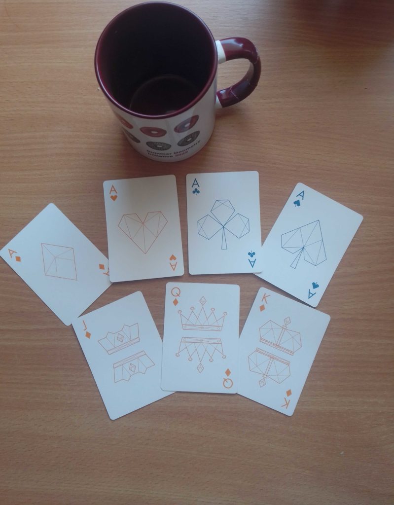
Selection of Cards from MathWorks’ Playing Cards…. and the SGI 2022 Mug.

For my first SGI blog, I have decided to combine what we have learned during the second day of the tutorial week given by the amazing Silvia Sellán to get an alternative version of the playing cards that we, fellows, have received in the swag package. The code can be found on SGI’s GitHub.

The cards are nicely designed already, so the goal is not to get a superior design but to put the knowledge we have collected into practice.

If you are curious about how the design was made by Mathworks, you can consult this website where they provide an explanation of the code that went into building the patterns. To briefly summarize the concept, the patterns were made using a Penrose Tiling, an aperiodic tiling that covers a surface with shapes such as triangles, polygons, etc. The Penrose Tiling is more distinct in larger surfaces where the tile’s repetition creates a distinct pattern.

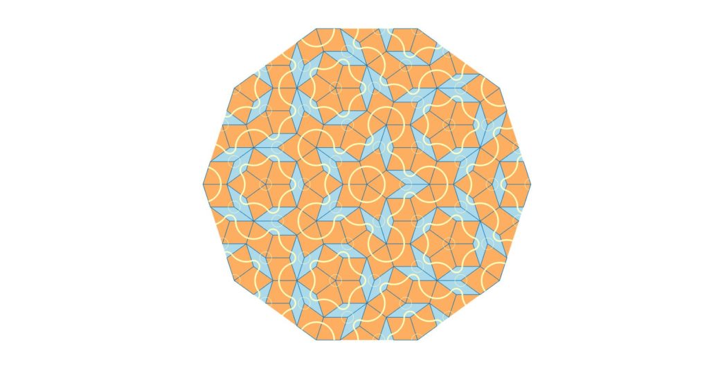
Penrose tiling as obtained after running the steps in the Playing Cards blog.

The tiling in the deck of playing cards is much simpler than what the Penrose Tiling usually ends up looking like because the number of tiles used to divide the shapes is very small. The aim is to recreate a simple pattern using triangulation principles that we have covered during the tutorial week.

The steps making our approach, which we are going to detail in this post, can be summarized in the pipeline below:

The idea used to recreate the cards is based on two commands, one of them being the drawing tool from the gpltoolbox and the triangulation tool:

[V,E,cid] = get_pencil_curves(1e-6); (1)

[U,G] = triangle(V,E,[],'Flags','-q30'); (2)

To recreate the style of the playing cards, we will need to transfer the drawing obtained in (1) to a polyline-based design. The drawing from get_pencil_curve is never straight, so we have to detect the existing segments and estimate their positions.

To achieve this polyline-based design, the position of the segment bounds and their connections are estimated which means that to recreate the polylines, we need to estimate the points that have corner properties and build the connections between these points.

To execute the step that consists of detecting these corner points, we can use the script find_corners.m. The principle is simple: a corner point is a point \(x_{i}\) where the sign of the derivative changes when measured between \(x_{i}\)’s predecessor \(x_{i-1}\) and successor \(x_{i+1}\). The edge cases where vertical lines exist in the drawing and that yield to +/-Inf derivatives and the case of horizontal lines that have a zero derivative along the segment are also accounted for.

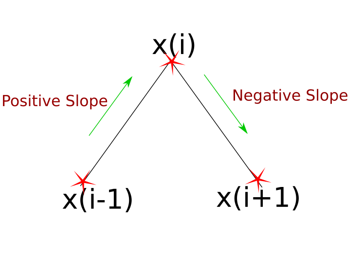
\(x_{i}\) is a corner with a change in the slope’s sign.

Points that satisfy this change in the slope’s sign will be considered corner candidates. At the end of the corner detection process, a pruning occurs to discard points that are very close to each other. Once we have these corner points, the polylines can be immediately seen as the connection between two consecutive corners.

Curvatures also naturally trigger this change in the slope’s sign. We do however need to distinguish between an intentional curvature and a non-intentional one caused by drawings which inherently have lines with varying degrees of curvature attributed to hand made drawings with the get_pencil_curve tool. This is solved by fixing a derivative threshold that discards very small variations.

When the polyline-based design is ready, we can run the triangulation tool as in (2) to obtain our resulting shapes.

In the pictures below, we have collected the results from our algorithm which generated triangulated polyline versions of shapes created by users. The results are not perfect due to many irregularities in the original drawing. These irregularities stem from the low quality of the drawings when using a mouse instead of an actual pen.

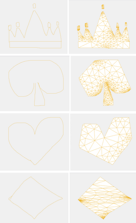
A queen, a spade, a heart and a diamond before and after triangulation.

Some interesting observations can be made from the results of the heart and spade shapes: the algorithm converts their curved lines into two straight lines which meet at a point that showcases corner properties which validates that strong curvatures are properly considered and the inevitable ones are discarded.

And with that, we can finally say that we have our own “artsy” playing cards design or maybe this could already be Mathworks’ design in a parallel universe!

Many of the SGI fellows experienced an error using the png2poly function from the gptoolbox: when applied to the example picture, the function throws an indexing error and in some cases makes Matlab crash. So, I decided to investigate the code.

The function png2poly transforms a png image into closed polylines (polygons) and applies a Laplacian smoothing operation. I found out that this operation was returning degenerated polygons, which later in the code was crashing Matlab.

But first, how does Laplacian smoothing work?

I had never seen how a smoothing operation works, and I was surprised with how simple the idea of Laplacian smoothing is. It’s an iterative operation, and at each iteration the positions of the vertices are updated using local information, the position of neighbor vertices.

New position of vertices after one iteration (credit: Stanford CS 468).

\[p_i \gets p_i + \frac{(p_{i+1} – p_i)}{2} + \frac{(p_{i-1} – p_i)}{2}\]

In polylines, every vertex has 2 neighbors, apart from boundary vertices, to which the operation is not applied. For closed polylines, Laplacian smoothing converges to a single point after many iterations.

The Laplacian matrix \(L\) can be used to apply the smoothing for the whole polyline at once, and a Lambda parameter (0 ≤ λ ≤ 1) can be introduced to control how much the vertices are going to move in one iteration:

\[p \gets p + \lambda L p\]

The best thing about Laplacian smoothing is that the same idea pleasantly applies for meshes in 3D! The difference is that in meshes every vertex has a variable number of neighbors, but the same formula using the Laplacian matrix can be used to implement it.

For more details on smoothing, check out this slide from Stanford, from which the images in this post were taken. It also talks about ways to improve this technique using an average of the neighbors weighted by curvature.

What about the bug?

The bug was the following: For some reason, the function that converts the png into polygons was generating duplicate vertices. Later in the code, a triangulate function is used on these polygons, and the duplicate vertices by themselves make the function crash. But even worse, when smoothing is applied to a polygon with duplicate vertices, strange things happen. Here’s an example of a square with 5 vertices (1 duplicated); after 3 iterations it becomes a non-simple polygon:

You can try to simulate the algorithm to see that it happens.

Also, the lambda parameter used was 1.0, which was too high, making small polygons collapse or generating new duplicate points, so I proposed 0.5 as the new parameter. For closed curves, Laplacian smoothing will converge to a single point, making the polygon really small after many iterations, which is also a problem for the triangulation function. In most settings, these converged polygons can be erased.

Some other problems were also found, but less relevant to be discussed here. A pull request was merged into the gptoolbox repository removing duplicate points and fixing the other bugs, and now the example used in the tutorial week should work just fine. The changes I made don’t guarantee that the smoothing operation is not generating self-intersection anymore, but for most cases it does.

Fun fact: There’s a technique for finding if a polygon has self-intersection called sweep line, which works in \(O(n\log n)\)—more efficient than checking every pair of edges!

The things I learned

Laplacian smoothing is awesome.
It’s really hard to build software for geometry processing that works properly for all kinds of input. You need to have complete control over degenerate cases, corner cases, precision errors, … the list goes on. It gets even harder when you want to implement something that depends on other implementations, that may by themselves break with certain inputs. Now I recognize even more the effort of professor Alec Jacobson and collaborators for creating gptoolbox and making it accessible.

Big thanks to Lucas Valença, for encouraging me to try and solve the bug, and to Dimitry Kachkovski, for testing my code.