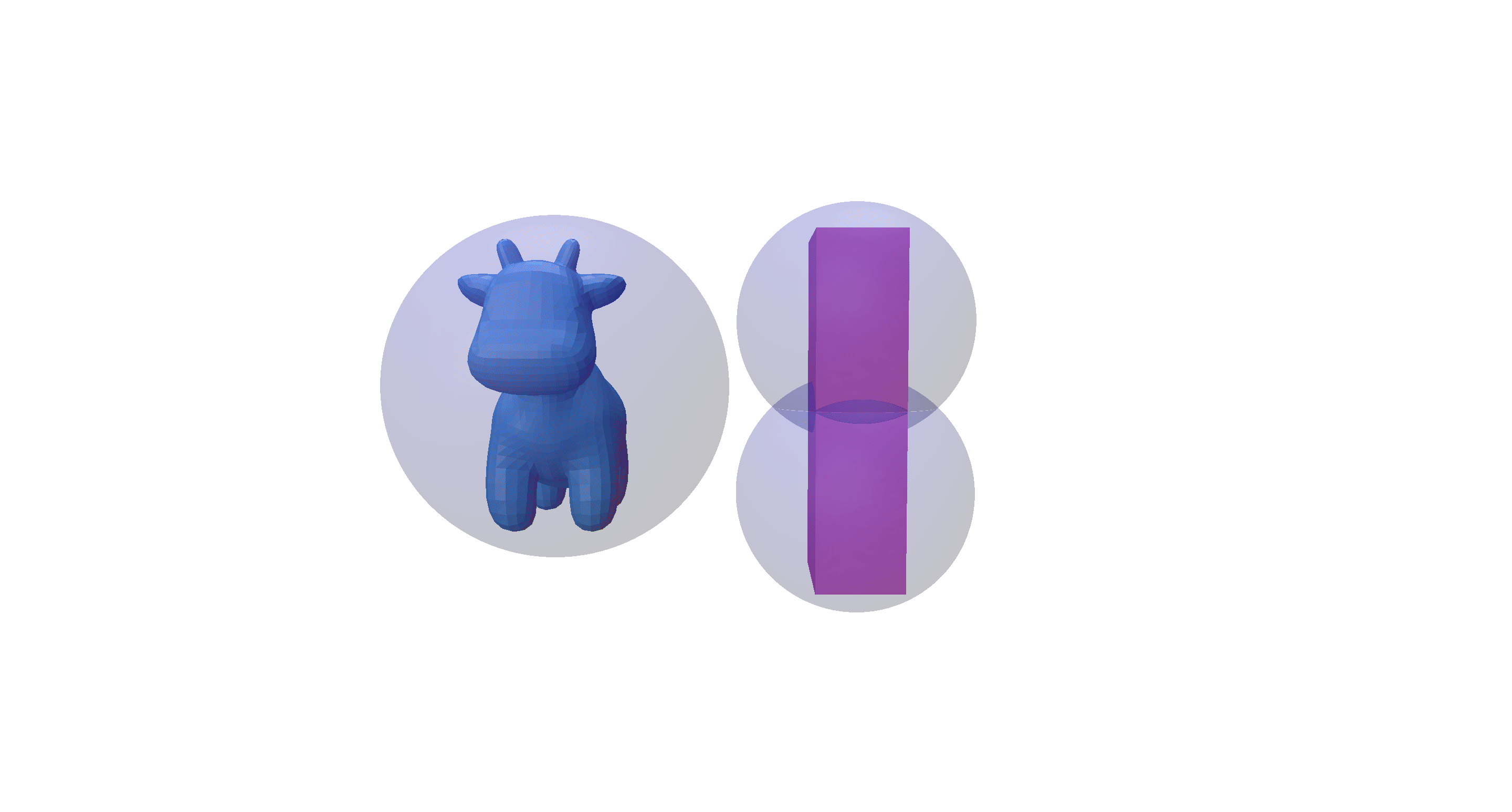
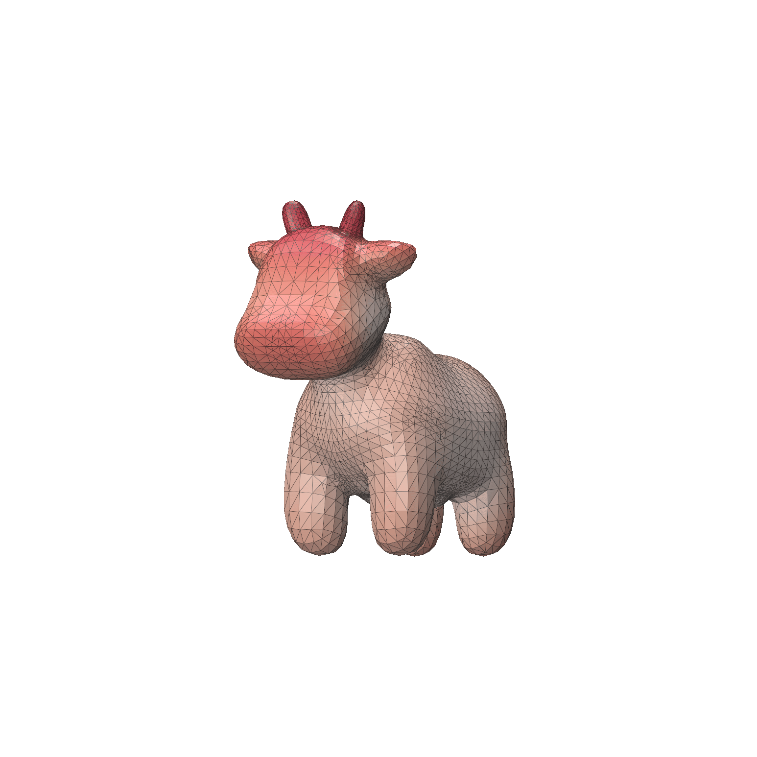
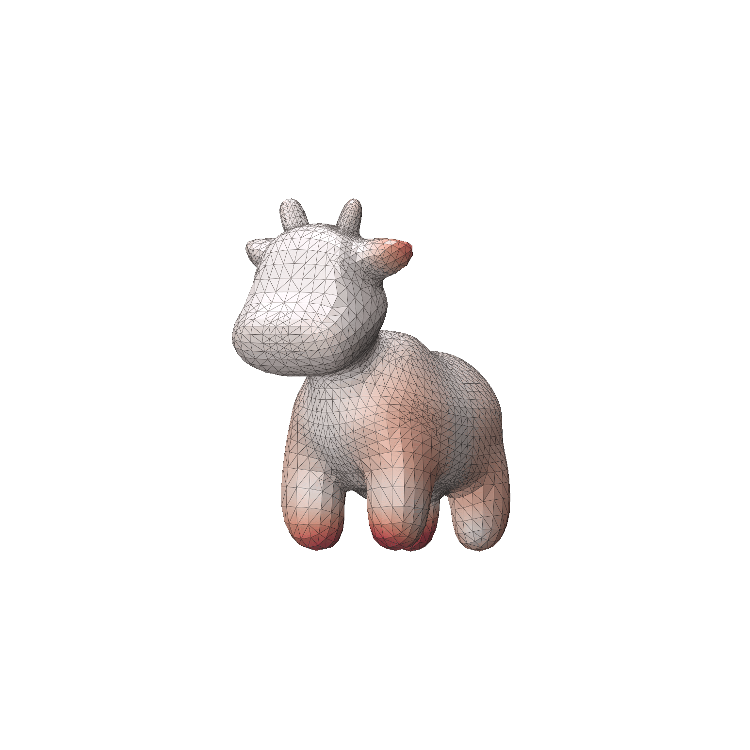
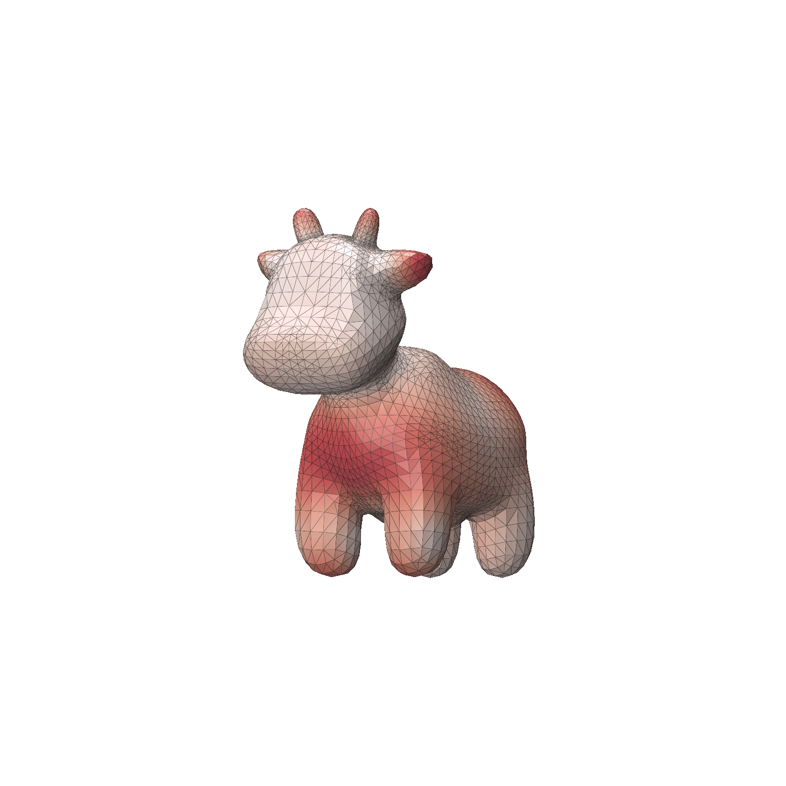
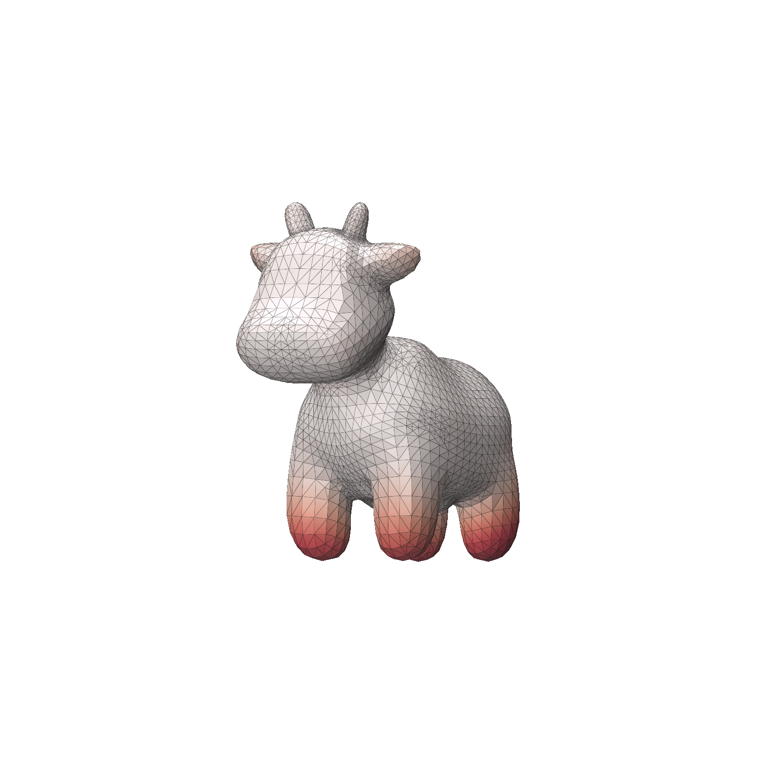
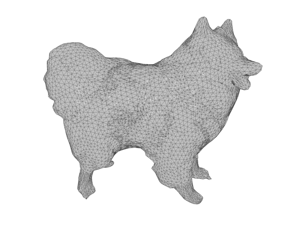
Figure 1: Our example 3D implementations of Gpytoolbox sweeping of Stanford bunny and Spot cow object across zig-zag trajectory
By Juan Parra, Kimberly Herrera, and Eleanor Wiesler
Project mentors: Silvia Sellán, Noam Aigerman
Introduction
Given a surface we can represent it moving along certain trajectory in space by a swept area or swept volume. It’s a good idea to take this approach to model 3D shapes or to detect a collision of the shape with another shape in its environment. There are several algorithms in the literature that address the construction of the surface of a swept volume in space, each taking their respective assumptions on the surface and the trajectory.
In our project we trained neural networks to predict the sweeping of a surface, and attempted to find the best representation of a neural network that deals with discontinuities that appear in the process.
Using Signed-Distance Functions to Model Shape Sweeping
By a swept volume we mean the trajectory that a solid moving through space made. The importance of representing a swept volume can go from art modeling to collision detection in robotics. We can model the swept volume of the solid motion as a surface in 3D. The goal of this project is to train neural networks to learn swept volumes, and so we conducted the experiments of this study using 2D shapes swept across a trajectory in the coordinate plane and evaluated resulting swept area. To study the trajectory or “sweeping” of these shapes, we used Signed Distance Functions (SDFs).
A signed distance function is a way to represent a closed orientable surface S in 3D (or a closed curve in 2D). This signed distance function (SDF) is given by a function:
\( D:\mathbb{R}^3\to\mathbb{R} \) such that \( |D(p)| = \min\{d(p,q)^2: q\in S\} \), and the sign of \( D(p) \) is negative if \( p \) is inside the surface and positive otherwise. The zero level set \( D^{-1}(0) \) is equal to the surface \( S \).
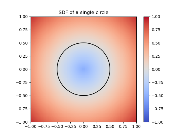
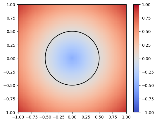
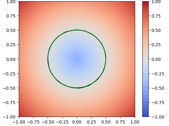
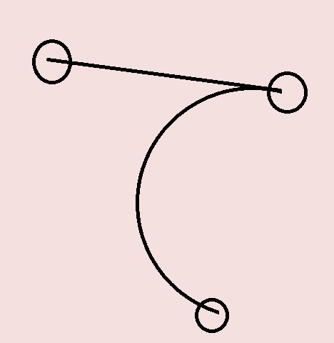
Given a signed distance function, we can use the Marching Cubes algorithm to construct a mesh representation of the surface. For example, \( G(x,y)=x^2 + y^2 -1 \) is the SDF of the unit circle.
Figure 1: SDF of a single circle
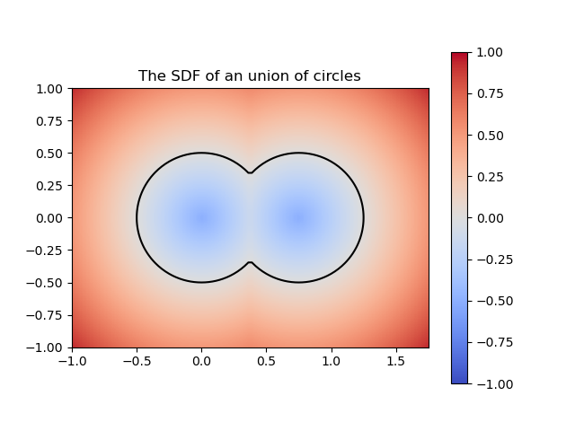
How to represent the SDF of the swept volume of a solid moving through space? We can leverage the operations between SDF’s to construct more complicated surfaces. For instance, the SDF of a unit circle is given by the function \( G(x,y) = x^2 + y^2 – 1 \) and the SDF of a translated circle to the right is \( H(x,y) = (x-0.75)^2 + y^2 – 1 \).
So if we wanted to paste both circles as if they were bubbles, we could define the union SDF as:
\[
\mathrm{union}(x,y)
=
\min\{
G(x,y), H(x,y)
\}
\]
Figure 2: SDF of a union of circles
If we want to perform a continuous motion of the solid we have to model it with a continuous function \(T: [0,1] \to SO(3)\) parametrized by the time, where
\(SO(3)\) is the set of rigid motions in 3D (abuse of notation to consider translations as well). Analogously we can think of rigid motions in 2D.
Suppose that \(F:\mathbb{R}^3 \to \mathbb{R}\) is the SDF of the solid we’re moving through space with the motion
\(T:[0,1] \to SO(3)\).
Then the swept volume of the solid is given by the SDF
$$
\text{swept volume}(\mathbf{x})
=
\min_{t\in[0,1]}
F(T_t^{-1}(\mathbf{x})).
$$
For the construction of a swept volume (or area) we can start with a previous
step, which is to define the function \(t^*:\mathbb{R}^3 \to \mathbb{R}\)
$$
t^*(\mathbf{x})
=
\mathrm{argmin}_{t\in [0,1]}
F(T_t^{-1}(\mathbf{x})),
$$
for which we will also have
$$
\text{swept volume}(\mathbf{x})
=
F
\left(
T_{t^*(\mathbf{x})}^{-1}
(\mathbf{x})
\right).
$$
The \(t^*\) function now it’s a “piecewise” continuous function on its domain
as shown in the following figures.
Finite Stamping
In order to compute an approximation for the swept volume, one first approach will be to make finite stamping of the SDF moving along a finite discretized sequence of times
\(0= t_1< \cdots< t_n=1\) and then compute the SDF
$$
\text{swept volume approximation}(\mathbf{x})
=
\min_{t\in \{t_1, \ldots, t_n\}}
F(T_t^{-1}(\mathbf{x})).
$$
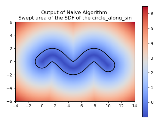
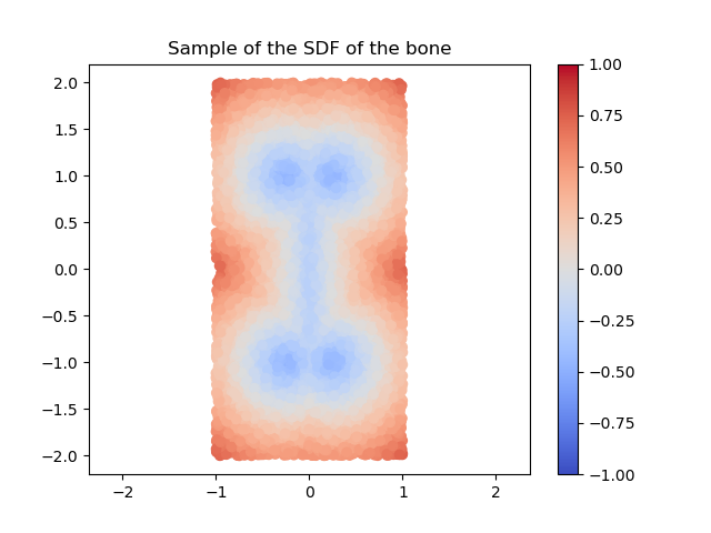
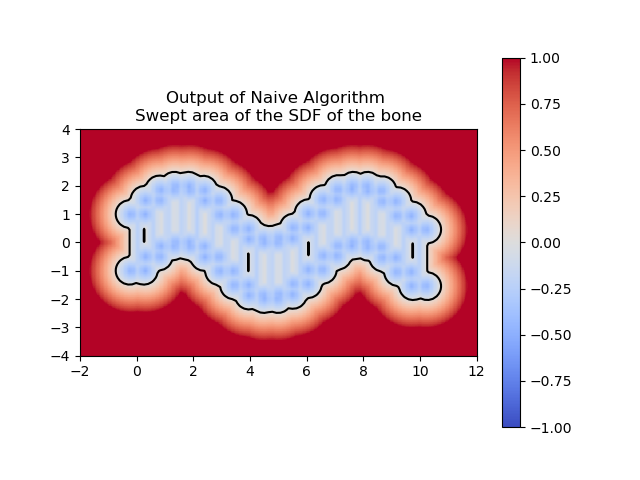
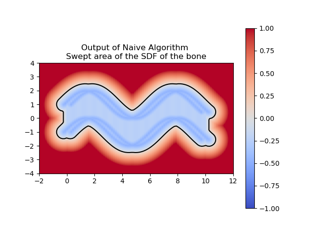
For example, if we define an SDF of a bone (see next 3 images),
and let's say we defined the motion \(T_t(x,y) = (x,y) + (t, \sin(t))\), then depending on how fine is our discretization, we can have a good or a bad approximation.
(a) 20 times
(b) 100 times
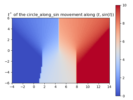
In this case we can also define an approximation to the \(t^*\) function as
follows
$$
t^*_{\text{approx}}(\textbf{x})
=
\text{argmin}_{t \in \{ t_1, \ldots, t_n \}}
F(T_{t}^{-1} (\mathbf{x})).
$$
However, we can notice that looking for the argument of the minimum
of a function can be computationally expensive, and that’s something we may want to do only once in our lifes.
Maybe we could substitute our Finite Stamping SDF with a neural network.
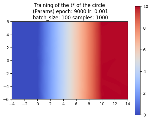
Knowing that \(t^*\) is not a continuous function, it will be interesting to fit a neural network to it, and play with its architecture so we find a neural network that represents better those discontinuities.
Learning Swept SDFs with Neural Networks
How to use a NN for SDFs
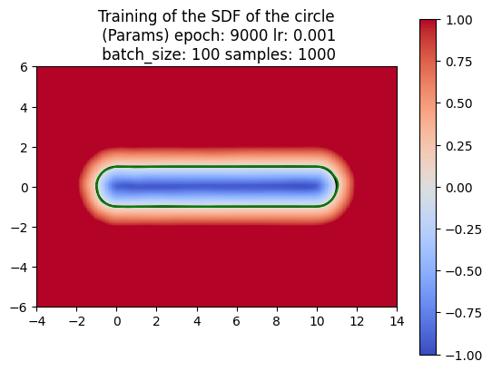
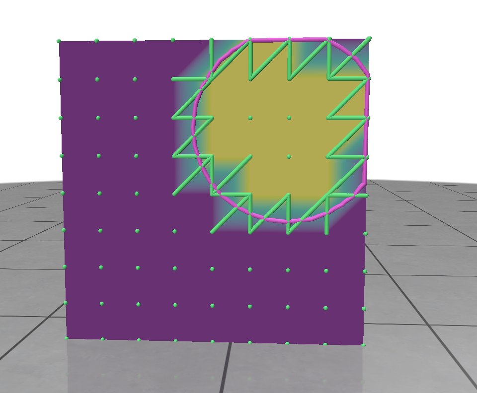
A neural network is just a function with many parameters; we can tweak these parameters to best approximate an SDF. To train the network, we first sample random points from the circle and compute their actual SDF values. The network’s goal is to predict these SDF values. By comparing the predicted values to the actual values using a loss function, the network can adjust its parameters to reduce the error. This adjustment is typically done through gradient descent, which iteratively refines the network’s parameters to minimize the loss. After training, we visualize the results to assess how well the neural network has learned to approximate the SDF. In the image below, the green represents the prediction for the circle by the neural network.
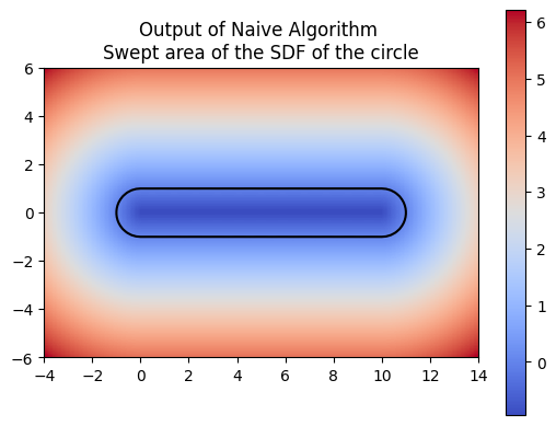
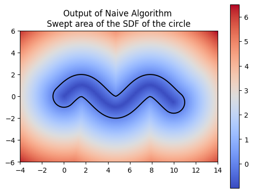
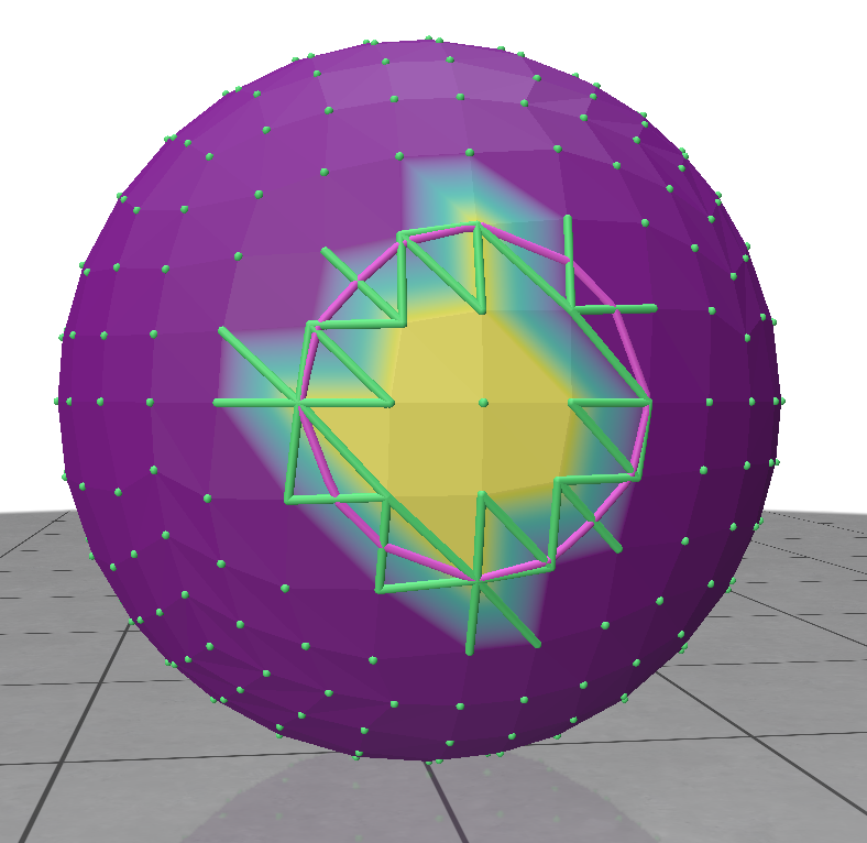
For computing a swept area, the neural network needs to approximate the union of multiple SDFs that together represent the swept area. Computing the swept area involves shifting the SDF along the trajectory at various points in time and then taking the union of all these SDFs. Once we understood how to compute the swept area ourselves, we had the neural network attempt the same. The following images show the results of our manual computation, which we refer to as the naive algorithm, for the sweeping of the circle along a horizontal path in comparison to the computation produced by the neural network. Similarly, the green represents the prediction for the swept area by the neural network.
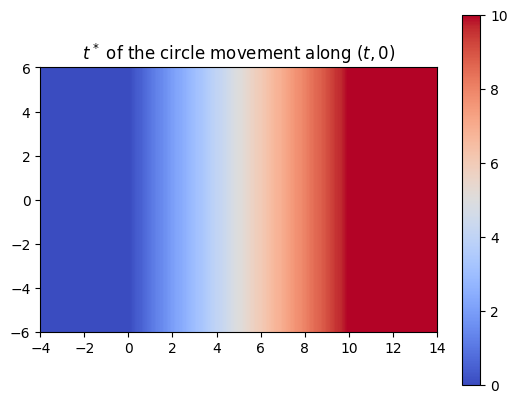
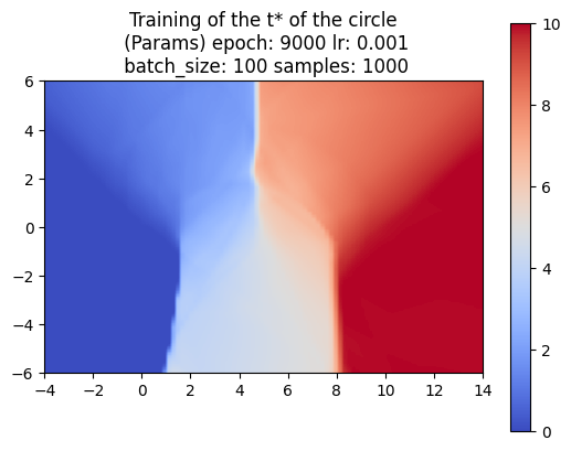
So far, we’ve trained the neural network to compute the SDF values for each point in a 2D grid. Now, since we are sweeping a shape over time, we want the network to return the times corresponding to these SDF values. We call these times t*. With the same shape and trajectory as above, the network has little issue doing this.
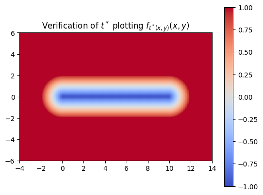
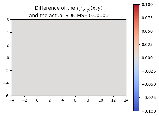
We also made sure that the t*‘s that we computed were producing the correct SDF of the swept area.
NN Difficulties detecting discontinuities
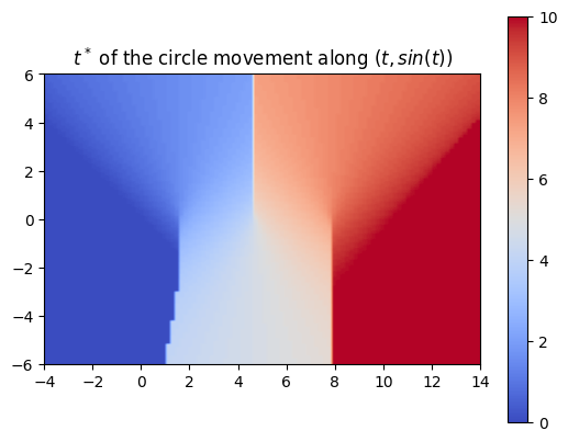
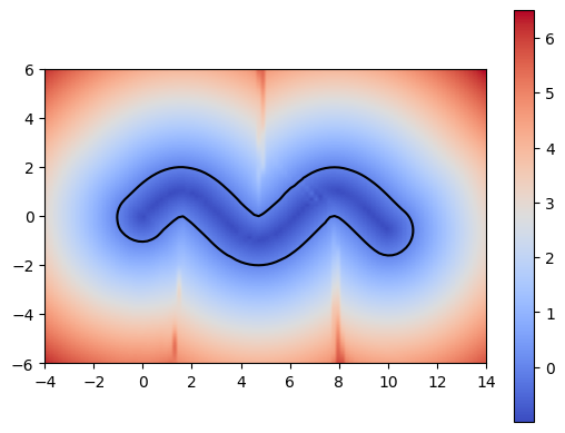
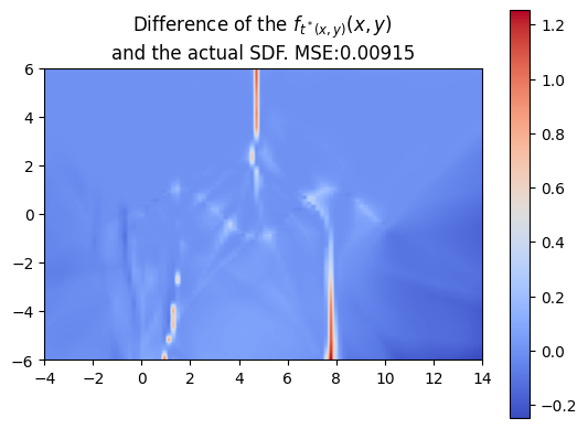
Using a more complex trajectory, such as a sine wave, introduces some challenges. While the neural network performs well in predicting the t* values, issues arise when computing the SDF with respect to these times. Specifically, the resulting SDF shows three lines emerging from the peaks and troughs of the curve. We can see this even more through the MSE plot.
The left image shows the sweeping of the circle using the t* values computed by the neural network.
These challenges become even more apparent when using shapes with sharper
edges such as a square. Because of this, we decided to work on optimizing the
neural network architecture.
Adjusting Our Neural Network Architecture
Changing Our Activation Function
Every neural network has a defined activation function. In the case of our preliminary neural network experiments above, the specified activation function was a Rectified Linear Unit (ReLU). Despite this, we did not achieve the most desirable outcome of minimal error in the predicted swept SDF versus the naive algorithm swept SDF. Specifically, we observed errors at sites of discontinuity, where there were changes in sign, for example.
In an attempt to improve neural network performance, we decided to experiment with different activation functions by altering our neural network architecture. Below, we present their corresponding results when used for swept SDF prediction.
Fellows: Sergius Justus Nyah, Nicolas Pigadas, Mutiraj Laksanawisit
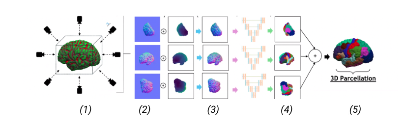
Picture 1: A high-level of the 2D projection descriptor pipeline we propose. (1) Extraction of multiple views and multiple descriptors from the 3D shape; (2) The extracted descriptors can be: normals, depth and curvature; (3) Input of the descriptors into a multi-view network; (4) Segmentation of the views (5) 3D reconstruction of the 3D segmented shape.
Abstract
Labeling brain surfaces is vital to many aspects of neuroscience and medicine, but to do so manually is laborious and time-consuming. An automated method would streamline the process, enabling more efficient analysis and interpretation of neuroimaging data. Such a task aligns with the longstanding inquiry in computer vision: is it more effective to use 3D shape representations or would 2D projection descriptor approaches yield better understanding of the shape? In this work, we explore the 2D approach of this question. We propose an automated end-to-end pipeline, structured into four main phases: selection of views for 2D projection extraction, rendering of the cortical mesh from multiple perspectives, segmentation of these projections and inverse rendering to map 2D segmentations back to 3D, integrating multiple views (Picture 1)
Definitions of Basic Project-Related Terms:
Pseudo-Rendering: This is a process whereby a 3D model, such as a cortical mesh (in our case), is projected into 2D images from multiple perspectives. This process involves a transformation from the 3D coordinate space to the 2D image plane. The perspectives can be defined by a virtual camera’s position and orientation relative to the 3D model. The resulting 2D images retain depth information from the 3D model, hence bringing forth the perception of three-dimensionality.
2D Segmentation: 2D Segmentation is the process of dividing a 2D image into distinct regions based on pixel characteristics such as color, intensity, or texture. The segmentation method, which can include techniques like thresholding, clustering, watershed, and edge-based methods, determines how these regions are defined. For example, in an image of an airplane in the sky, one region might be the blue sky and another the white airplane. Similarly, an image of a chair could be segmented into regions representing the chair’s legs, seat, and backrest. Post-processing steps may be applied to refine these regions. The success of the segmentation can be evaluated using metrics like pixel accuracy, Intersection over Union (IoU), and Dice coefficient (a measure of the performance of Segmentation algorithms).
Cortical Mesh: This is a 3D model that represents the outer surface of the brain (cerebral cortex), usually obtained from Magnetic Resonance Imaging data.
Parcellation: This refers to the process of dividing cortical meshes, typically derived from brain imaging data, into distinct regions or parcels. These parcels often represent functionally or structurally distinct areas of the brain. Its purpose here is to simplify the analysis of brain imaging data by reducing the complexity of the data and focusing on regions of interest.
Initial Steps:
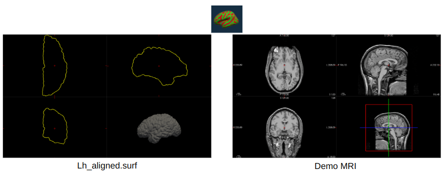
Load and visualize Brain surfaces with FreeSurfer [Link]
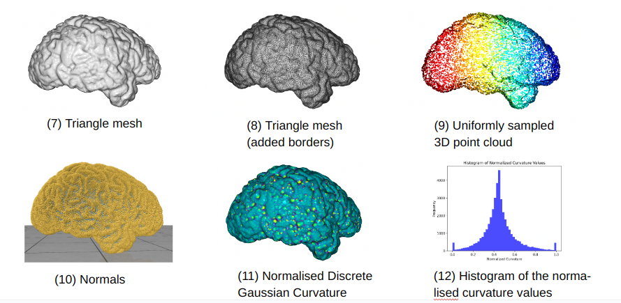
Compute Normals, Curvature, and Point clouds from the Mesh surface
Method:
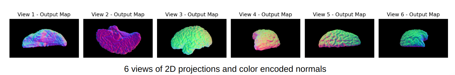
Selecting camera views to Extract 2D Images.
The selection of camera views is a critical step which involves determining the optimal perspectives from which to project the 3D cortical mesh onto 2D planes. Our goal here is to capture the most informative views that will facilitate accurate segmentation and subsequent inverse rendering.
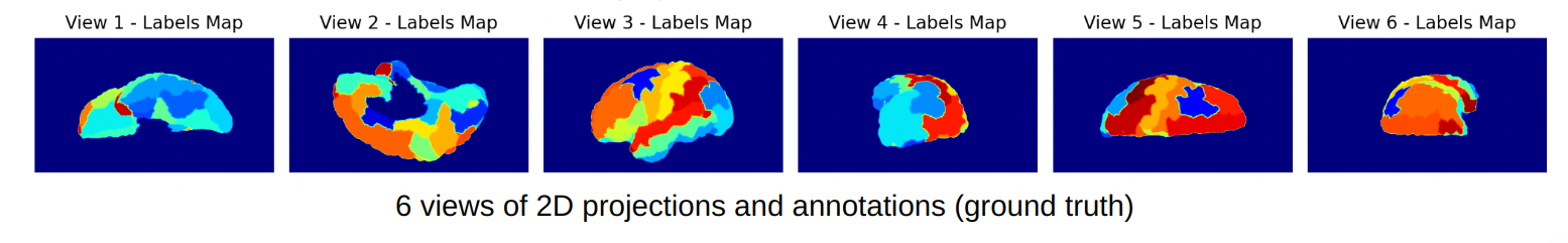
We will start adopting a systematic approach to select six canonical views: Front, Bottom, Top, Right, Back, and Left. These views are chosen to ensure comprehensive coverage of the cortical surface, capturing its intricate geometry from multiple angles.
The selection process begins by computing the intrinsic matrix for the camera, which is used to simulate the camera’s perspective. The intrinsic matrix is calculated using the following function in Python:
def compute_intmat(img_width, img_height):

    intmat = np.eye(3)

    # Fill the diagonal elements with appropriate values
    np.fill_diagonal(intmat, [-(img_width + img_height) / 1, -(img_width + img_height) / 1, 1])

    # Set the last column of the matrix for image centering
    intmat[:,-1] = [img_width / 2, img_height / 2, 1]

    return intmat
Next, we’ll create external transformation matrices to align the camera with the six predefined views. These matrices help us generate rays for ray casting, allowing us to simulate what the camera would see from each perspective. We’ll use the pinhole camera model to generate these rays.
By casting rays from these six perspectives, we can project the entire cortical surface onto 2D planes, making sure we capture all the important features. This multi-view approach strengthens the segmentation process by reducing the chances of occlusions and giving us a more complete picture of the 3D structure.
The following images illustrate the six canonical views we used in our pipeline:
Now, We will accompany each 2D projection with annotations (ground truth).
These views are crucial for the next steps in our pipeline, such as rendering, segmentation, and inverse rendering. By carefully choosing and using these perspectives, we improve both the accuracy and efficiency of the automated labeling process. The six camera positions ensure that every part of the cortical surface is captured, giving us a complete set of 2D projections that can be accurately mapped back to the 3D structure.
2D Projections: Annotations and Curvature
To continue, we take the 2D projections obtained from the six camera views and perform annotations and curvature calculations, which are essential for understanding the cortical surface’s geometry and features.
Process:
Calculate the curvature of the cortical surface from the 2D projections, which helps in identifying important features and understanding the surface’s geometry.
Annotate the 2D projections with relevant labels, such as different brain regions or anatomical landmarks.
Use these annotations to the CNN (As seen below) for automated labeling.
Code:
# Compute per-face curvature using gpytoolbox (angle defect)
curvature = gpy.angle_defect(vertices, faces)


# Debugging: Print raw curvature values
print("Raw Curvature Values:")
print(curvature)
print("Curvature min:", np.min(curvature))
print("Curvature max:", np.max(curvature))


# Percentile-based normalization
lower_percentile = np.percentile(curvature, 1)
upper_percentile = np.percentile(curvature, 99)


# Clipping the curvature values to the 1st and 99th percentiles to diminish the effect of outliers
curvature_clipped = np.clip(curvature, lower_percentile, upper_percentile)


# Normalize the clipped curvature values between 0 and 1
curvature_normalized = (curvature_clipped - lower_percentile) / (upper_percentile - lower_percentile)


# Debugging: Print normalized curvature values
print("Normalized Curvature Values:")
print(curvature_normalized)


# Select color map
color_map = plt.get_cmap('viridis')
curvature_colors = color_map(curvature_normalized)[:, :3] # Ignore alpha channel


# Create Open3D mesh
mesh = o3d.geometry.TriangleMesh()
mesh.vertices = o3d.utility.Vector3dVector(vertices)
mesh.triangles = o3d.utility.Vector3iVector(faces)
mesh.vertex_colors = o3d.utility.Vector3dVector(curvature_colors) # Apply colors to vertices


# Compute normals to improve lighting in visualization
mesh.compute_vertex_normals()


# Visualize the mesh with curvature coloring
o3d.visualization.draw_geometries([mesh], window_name='Mesh with Curvature Colors')


# Visualize the normalized curvature values as a histogram
plt.figure()
plt.hist(curvature_normalized, bins=50, color='blue', alpha=0.7)
plt.title("Histogram of Normalized Curvature Values")
plt.xlabel("Normalized Curvature")
plt.ylabel("Frequency")
plt.show()
Result (As seen also in (2) above):
Training the multi-view CNN
Now we use the annotated 2D projections to train a multi-view Convolutional Neural Network (CNN). This multi-view CNN leverages the different perspectives to improve the accuracy of the labeling process.
Process:
Data Preparation:
Prepare the annotated 2D projections as input data for the CNN.
Split the data into training, validation, and test sets.
import os
import nibabel as nib
import torch
from torch.utils.data import Dataset, DataLoader

def load_data(data_dir):

    data = []
    labels = []

    for subject_dir in os.listdir(data_dir):
        surf_dir = os.path.join(data_dir, subject_dir, 'surf')
        label_dir = os.path.join(data_dir, subject_dir, 'label')

        if os.path.isdir(surf_dir) and os.path.isdir(label_dir):
            # Load surface data
            surf_file = os.path.join(surf_dir, 'lh_aligned.surf')
            if os.path.exists(surf_file):
                surf_data = nib.freesurfer.read_geometry(surf_file)[0]
                data.append(surf_data)

            # Load label data
            label_file = os.path.join(label_dir, 'lh.annot')
            if os.path.exists(label_file):
                label_data = nib.freesurfer.read_annot(label_file)[0]
                labels.append(label_data)

    return np.array(data), np.array(labels)


# Load actual data
train_data, train_labels = load_data('/home/sergy/cortical-mesh-parcellation/10brainsurfaces (1)')
val_data, val_labels = load_data('/home/sergy/cortical-mesh-parcellation/10brainsurfaces (1)')


# Convert data to PyTorch tensors
train_data = torch.tensor(train_data, dtype=torch.float32)
train_labels = torch.tensor(train_labels, dtype=torch.long)
val_data = torch.tensor(val_data, dtype=torch.float32)
val_labels = torch.tensor(val_labels, dtype=torch.long)


# Define custom dataset class
class ExampleDataset(Dataset):
    def __init__(self, data, labels):
        self.data = data
        self.labels = labels

    def __len__(self):
        return len(self.data)

    def __getitem__(self, index):
        return self.data[index], self.labels[index]


# Create DataLoader for training and validation data
train_dataset = ExampleDataset(train_data, train_labels)
val_dataset = ExampleDataset(val_data, val_labels)

train_loader = DataLoader(train_dataset, batch_size=32, shuffle=True)
val_loader = DataLoader(val_dataset, batch_size=32, shuffle=False)
2. Model Architecture:
Design a CNN architecture that can handle multi-view inputs.
Use techniques like data augmentation to improve the model’s robustness.
from trainCNN import MultiViewCNN
import torch.nn as nn

# Initialize the model
model = MultiViewCNN()

# Define the loss function and optimizer
criterion = nn.CrossEntropyLoss()
optimizer = torch.optim.Adam(model.parameters(), lr=0.001)
3. Training the CNN:
Train the CNN using the prepared data.
Monitor the training process using metrics like accuracy and loss.
# Training loop
for epoch in range(5): # 5 epochs
model.train()
for i, (inputs, labels) in enumerate(train_loader):
optimizer.zero_grad()
outputs = model(inputs)
loss = criterion(outputs, labels)
loss.backward()
optimizer.step()
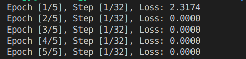
if i % 100 == 0:
print(f"Epoch [{epoch+1}/5], Step [{i+1}/{len(train_loader)}], Loss: {loss.item():.4f}")
# Validation loop
model.eval()
val_loss = 0.0
with torch.no_grad():
for inputs, labels in val_loader:
outputs = model(inputs)
loss = criterion(outputs, labels)
val_loss += loss.item()
val_loss /= len(val_loader)
print(f"Validation Loss after Epoch [{epoch+1}/5]: {val_loss:.4f}")
Training result:
Analysis of Training Results:
Initial Loss: In the first epoch, the initial loss is 2.3174. This indicates that the model is starting to learn from the data, but there is still a significant difference between the predicted and actual labels.
Subsequent Epochs: From the second epoch onwards, the loss drops to 0.0000. This suggests that the model has quickly learned to minimize the loss and make accurate predictions.
3D Reconstruction: Annotations and Curvature:
To conclude, we will map the 2D annotations and curvature back to the 3D structure, which provides a comprehensive view of the cortical surface with detailed annotations and curvature information. We can divide this into 3 steps;
Mapping Annotations:
Firstly, we will map the annotations predicted by the Multi-View CNN back to the 3D cortical surface, which involves projecting the 2D annotations onto the 3D mesh.
import numpy as np
def map_annotations_to_3d(annotations_2d, vertices, faces):
    # Initialize a 3D array to store the annotations
    annotations_3d = np.zeros(vertices.shape[0])
    # Iterate over each face and map the 2D annotations to the 3D vertices
    for i, face in enumerate(faces):
        for vertex in face:
            annotations_3d[vertex] = annotations_2d[i]
    return annotations_3d
# Example usage
annotations_2d = np.random.randint(0, 10, size=(faces.shape[0],))  # Replace with actual 2D annotations
annotations_3d = map_annotations_to_3d(annotations_2d, vertices, faces)
2. Mapping Curvature:
We then map the calculated curvature values from the 2D projections back to the 3D surface. This will help us in visualizing the curvature on the 3D model.
def map_curvature_to_3d(curvature_2d, vertices, faces):
    # Initialize a 3D array to store the curvature values
    curvature_3d = np.zeros(vertices.shape[0])

    # Iterate over each face and map the 2D curvature to the 3D vertices
    for i, face in enumerate(faces):
        for vertex in face:
            curvature_3d[vertex] = curvature_2d[i]

    return curvature_3d

# Define vertices and faces
vertices = np.array([[0, 0, 0], [1, 0, 0], [1, 1, 0], [0, 1, 0]])
faces = np.array([[0, 1, 2], [0, 2, 3]])
3. Integration and Visualization:
Finally, we will integrate the annotations and curvature into a single 3D model and use a visualization tool (Polyscope, in this case) to display the final annotated and curved 3D structure.
# Load annotations and curvature data
annotations_path = '10brainsurfaces (1)/100206/label/lh.annot'
curvature_path = 'curvature_array.npy'
annotations_3d = nib.freesurfer.read_annot(annotations_path)[0]
curvature_3d = np.load(curvature_path)
# Ensure curvature_3d has the correct shape
if curvature_3d.shape[0] != vertices.shape[0]:
    curvature_3d = curvature_3d[:vertices.shape[0]]
# Initialize Polyscope
ps.init()

# Register the 3D mesh with Polyscope
mesh = ps.register_surface_mesh("annotated_brain", vertices, faces)
# Add the annotations and curvature as scalar quantities
mesh.add_scalar_quantity("annotations", annotations_3d, defined_on="vertices", cmap="viridis")
mesh.add_scalar_quantity("curvature", curvature_3d, defined_on="vertices", cmap="coolwarm")
# Show the visualization
ps.show()
Final Results from Annotations and Mappings:
Our pipeline successfully achieved its goals:
The trainCNN script trained the MultiViewCNN model and saved the state dictionary.
The projections.py script visualized the cortical mesh with annotations and curvature, as seen below
The trained model extracted features from the 2D projections, enhancing our understanding of the cortical surface.
Our goal of Pseudo Rendering was achieved.
Figure 1: Front view of brain section with labeled annotations:
Figure 2: Back view of brain section with labeled annotations:
To conclude this long post, permit us discuss the practical use-scopes of Pseudo rendering, across diverse feilds in Science, healthcare, and Research:
Pseudo-rendering enhances the visualization of complex anatomical structures, aiding in better diagnosis and treatment planning by providing detailed 3D models of organs and tissues.
Enables efficient analysis of 3D data by generating 2D projections from multiple camera angles, like in the case of cortical mesh parcellation.
Reduces computational resources required for rendering complex 3D models, making the process less resource-intensive.
Supports interactive exploration of 3D models, allowing users to manipulate 2D projections to explore different views and perspectives.
Closing Remarks:
At this point, we would like to express our gratitude to our amazing mentor, Dr. Karthik Gopinath, and volunteer mentor, Kyle Onghai, for their unwavering support and guidance throughout the project. Their effective guidance enabled us to rapidly develop our ideas and foster a deep passion for the project. We look forward to continuing our work on this brilliant research idea as soon as possible.
Project Mentors: Sainan Liu, Ilke Demir and Alexey Soupikov
Previously, we introduced 3D Gaussian Splatting and explained how this method proposes a new approach to view synthesis. In this blog post, we will talk about how 3D Gaussian splatting [1] can be further extended to enable potential applications to reconstruct both the 3D and the dynamic (4D) world surrounding us.
We live in a 3D world and use natural language to interact with this world in our day to day lives. Until recently, 3D computer vision methods were being studied on closed set datasets, in isolation. However, our real world is inherently open set. This suggests that the 3D vision methods should also be able to extend to natural language that could accept any type of language prompt to enable further downstream applications in robotics or virtual reality.
Gaussians with Semantics
A recent trend among the 3D scene understanding methods is therefore to recognize and segment the 3D scenes with text prompts in an open-vocabulary [1,2]. While being relatively new, this problem have been extensively studied in the past year. However, these methods still investigate the semantic information within 3D scenes through an understanding point of view — So, what about reconstruction?
1. LangSplat: 3D Language Gaussian Splatting (CVPR2024 Highlight)
One of the most valuable extensions of the 3D Gaussians is the LangSplat [3] method. The aim here is to incorporate the semantic information into the training process of the Gaussians, potentially enabling a coupling between the language features and the 3D scene reconstruction process.
Figure 1. Framework of LangSplat [3].
The framework of LangSplat consists of three main components which we explain below.
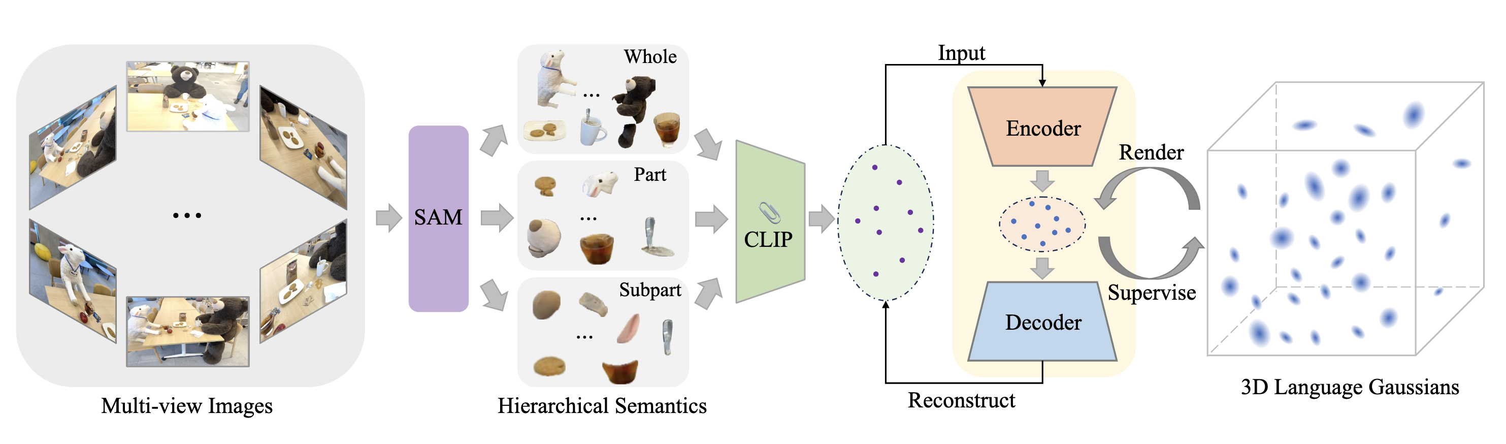
1.1 Hierarchical Semantics
LangSplat not only considers the objects within the scene as a whole but also learns the hierarchy to enable “whole”, “part” and “subpart”. This three levels of hierarchy is achieved by utilizing a foundation model (SAM [4]) for image segmentation. Leveraging SAM, enables precise segmentation masks to effectively partition the scene into semantically meaningful regions. The redundant masks are then removed for each of these three sets (i.e. whole, part and subpart) based on the predicted IoU score, stability score, and overlap rate between masks.
Next step is then to associate each of these masks in order to obtain pixel-aligned language features. For this, the framework makes use of a vision-language model (CLIP [5]) to extract an embedding vector per image region that can be denoted as:
$$ \boldsymbol{L}_t^l(v)=V\left(\boldsymbol{I}_t \odot \boldsymbol{M}^l(v)\right), l \in\{s, p, w\}, (1) $$
where \(\boldsymbol{M}^l(v)\) represents the mask region to which pixel $v$ belongs at the semantic level \(l\).
The three levels of hierarchy eliminates the need for search upon querying, making the process more efficient for downstream tasks.
1.2 3D Gaussian Splatting for Language Fields
Up until now, we have talked about semantic information extracted from multi-view images mainly in 2D \(\left\{\boldsymbol{L}_t^l, \mid t=1, \ldots, T\right\}\). We can now use these embeddings to learn a 3D scene which models the relationship between 3D points and 2D pixel-aligned language features.
LangSplat aims to augment the original 3D Gaussians [1] to obtain 3D language Gaussians. Note that at this point, we have pixel aligned 512-dimensional CLIP features which increases the space-time complexity. This is because CLIP is trained on internet scale data (\(\sim\)400 million image and text pairs) and the CLIP embeddings space is expected to align with arbitrary image and text prompts. However, our language Gaussians are scene-specific which suggests that we can compress the CLIP features to enable a more efficient and scene-specific representation.
To this end, the framework trains an autoencoder trained with a reconstruction objective on the CLIP embeddings \(\left\{\boldsymbol{L}_t^l\right\}\) with L1 and cosine distance loss:
where \(d_{ae}(.)\) denotes the distance function used for the autoencoder. The dimensionality of the features are then reduced from \(D=512\) to \(d=3\) with high memory efficiency.
Finally, the language embeddings are optimized with the following objective to enable 3D language Gaussians:
$$\mathcal{L}_{\text {lang }}=\sum_{l \in\{s, p, w\}} \sum_{t=1}^T d_{l a n g}\left(\boldsymbol{F}_t^l(v), \boldsymbol{H}_t^l(v)\right), (3) $$
where \(d_{lang}(.)\) denotes the distance function.
1.3 Open-vocabulary Querying
The learned 3D language field can easily support open-vocabulary 3D queries, including open-vocabulary 3D object localization and open-vocabulary 3D semantic segmentation. Due to the three levels of hierarchy, each text query will be associated with three relevancy maps at each semantic level. In the end, LangSplat chooses the level that has the highest relevancy score.
Our Results
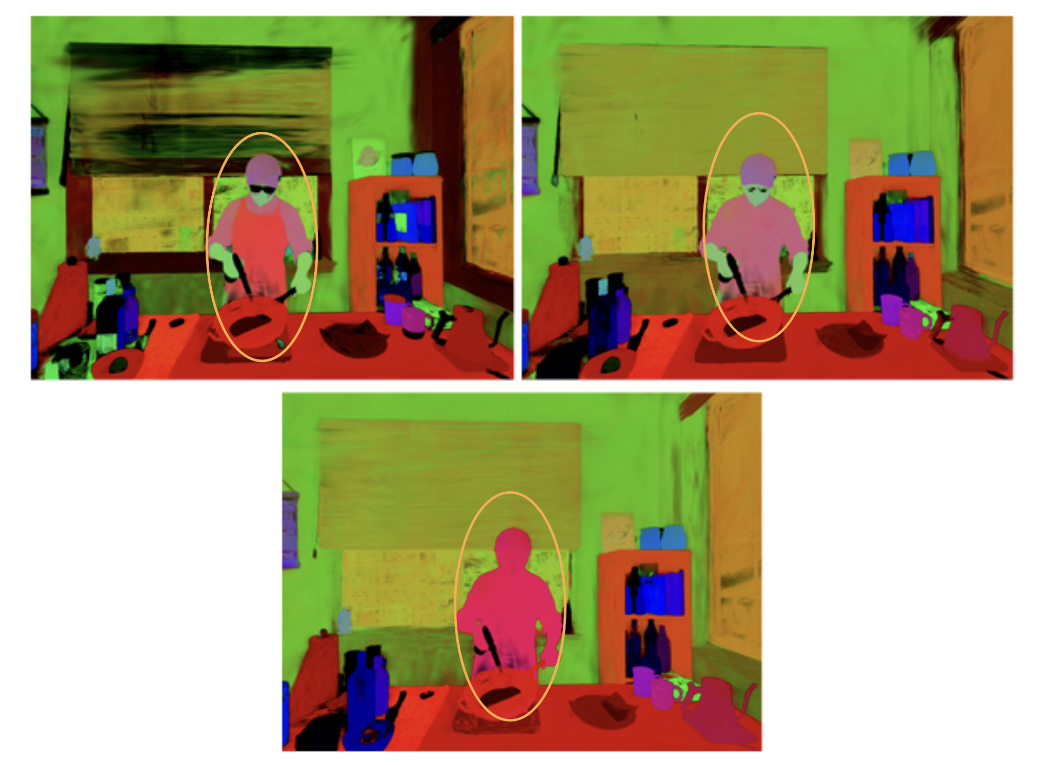
Following the previous blog post, we run LangSplat on the initial frames of the flaming salmon scene of the Neu3D dataset and share both the novel view renderings and the visualization of language features per each level of hierarchy:
Figure 2. Results of LangSplat for the initial frames of the flaming salmon scene on Neu3D dataset for three levels of semantic hierarchy.
Figure 3. Results of LangSplat for the inital frames of the flaming salmon scene on Neu3D dataset across multiple views for the same level of hierarchy.
Gaussians in 4D
Another extension of the 3D Gaussian splatting involves incorporating Gaussians to dynamic settings. The previously discussed dataset, Neu3D, enables a study to move from novel view synthesis for static scenes to reconstructing Free-Viewpoint Videos, or FVVs in short. The challenge here, comes from the additional time component that can pose further illumination or brightness changes. Furthermore, objects can change their look or form across time and new objects that were not present in the initial frames can later emerge in the videos. Not only this, but also the additional frames per view (1200 frames per camera view in Neu3D) highlights once again the importance of efficiency to enable further applications.
In comparison to language semantics, Gaussian splatting methods in the fourth dimension have been investigated more in detail. Before moving on with our selected method, here we highlight the most interesting works for interested readers:
4D Gaussian Splatting for Real-Time Dynamic Scene Rendering
3DGStream: On-the-Fly Training of 3D Gaussians for Efficient Streaming of Photo-Realistic Free-Viewpoint Videos
Spacetime Gaussian Feature Splatting for Real-Time Dynamic View Synthesis
2. 3DGStream: On-the-Fly Training of 3D Gaussians for Efficient Streaming of Photo-Realistic Free-Viewpoint Videos (CVPR 2024 Highlight)
As discussed above, constructing photo-realistic FVVs of dynamic scenes is a challenging problem. While existing methods address this, they are bounded by an offline training scenario, meaning that they would require the presence of future frames in order to perform the reconstruction task. We therefore consider 3DGStream [7], due to its ability of online training.
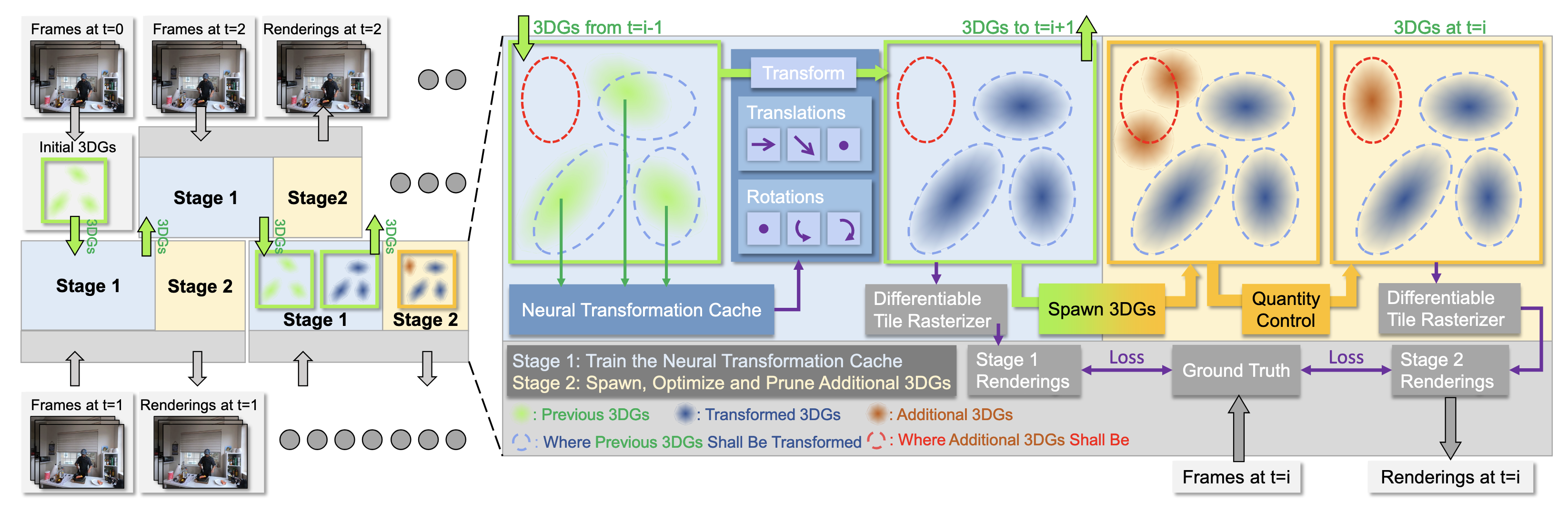
3DGStream eliminates the requirement of long video sequences and instead performs on-the-fly construction for real-time renderable FVVs on video streams. The method consists of two main stages that involve the Neural Transformation Cache and the optimization of 3D Gaussians for the next time step.
Figure 4. Overview of 3DGStream [7].
2.1 Neural Transformation Cache (NTC)
NTC enables a compact, efficient, and adaptive way to model the transformations of 3D Gaussians. Following I-NGP [8], the method uses a multi-resolution hash encoding together with a shallow fully-fused MLP. This encoding essentially uses multi-resolution voxel grids that represent the scene and the grids are mapped to a hash table storing a \(d\)-dimensional learnable feature vector. For a given 3D position \(x \in \mathcal{R}^3\), its hash encoding at resolution $l$, denoted as \(h(x; l) \in \mathcal{R}^d\), is the linear interpolation of the feature vectors corresponding to the eight corners of the surrounding grid. Then, the MLP that enhances the performance of the NTC can be formalized as
$$ d \mu, d q=M L P(h(\mu)), (4) $$
where $\mu$ denotes the mean of the input 3D Gaussian. The mean, rotation and SH (spherical harmonics) coefficients of the 3D Gaussian are then transformed with respect to \(d\mu\) and \(dq\).
At Stage 1, the parameters of NTC are optimized following the original 3D Gaussians with \(L_1\) combined with a D-SSIM term:
$$ L=(1-\lambda) L_1+\lambda L_{D-S S I M} (5) $$
Additionally, 3DGStream employs an additional NTC warm up which uses the loss given by: $$ L_{w a r m-u p}=||d \mu||_1-\cos ^2(\text{norm}(d q), Q), (6) $$ where \(Q\) is the identity quaternion.
2.2 Adaptive 3D Gaussians
While 3D Gaussians transformations perform relatively well for dynamic scenes, they fall short when new objects that were not present in the initial time steps emerge later in the video. Therefore, it is essential to add new 3D Gaussians to model the new objects in a precise manner.
Based on this observation, 3DGStream aims to spawn new 3D Gaussians in regions where gradient is high. To be able to capture every region where a new object might potentially occur, the method uses an adaptive 3D Gaussian spawn strategy. To elaborate, view-space positional gradient during the final training epoch of Stage 1 is tracked, and at the end of this stage, 3D Gaussians with an average magnitude of view-space position gradients exceeding a low threshold \(\tau_{grad} = 0.00015\) are selected. For each of these selected 3D Gaussians, the position of the additional Gaussian is sampled from \(X \sim N (\mu, 2\sigma)\), where μ and Σ is the mean and the covariance matrix of the selected 3D Gaussian.
However, this may result in emerging Gaussians to quickly become transparent, failing to capture the emerging objects. To address this, SH coefficients and scaling vectors of these 3D Gaussians are derived from the selected ones, with rotations set to the identity quaternion \(q = [1, 0, 0, 0]\) with opacity 0.1. After the spawning process, the 3D Gaussians undergo an optimization utilizing the loss function (Eq. (5)) as introduced in Stage 1.
At the Stage 2, an adaptive 3D Gaussian quantity control is employed to make sure that Gaussians grow reasonably. For this reason, a high threshold of \(\tau_\alpha = 0.01\) is set for the opacity value. At the end of each epoch, new 3D Gaussians are spawned for the Gaussians where view-space position gradients exceed \(\tau_{grad}\). The spawned Gaussians inherit the rotations and SH coefficients from the original 3D Gaussians but have an adjusted scale to 80%. Finally, any 3D Gaussian with opacity values below \(\tau_{\alpha}\) are discarded to control the growth of the quantity of total number of Gaussians.
Our Results
We setup and replicate the experiments of 3DGStream on the flaming salmon scene of Neu3D.
Figure 5. Results of 3DGStream for flaming salmon scene of Neu3D. While the transformed 3D Gaussians remain consistent, we see that the challenge with newly emerging objects (e.g. flames) remains.
Next Steps
Figure 6. Results on multi-view consistency of video foundation models on the flaming salmon scene of Neu3D.
To get the best of both worlds, our aim is to integrate the semantic information as in LangSplat [4] into dynamic scenes. We would like to achieve this by utilizing foundation models for videos to enable static and dynamic scene separation to construct free-viewpoint videos. We believe that this could enable further real world applications in the near future.
References
[1] Kerbl, B., Kopanas, G., Leimkühler, T., & Drettakis, G. 3D Gaussian Splatting for Real-Time Radiance Field Rendering. ACM Trans. Graph. (SIGGRAPH) 2023. [2] Takmaz, A., Fedele, E., Sumner, R., Pollefeys, M., Tombari, F., & Engelmann, F. OpenMask3D: Open-Vocabulary 3D Instance Segmentation. NeurIPS 2024. [3] Nguyen, P., Ngo, T. D., Kalogerakis, E., Gan, C., Tran, A., Pham, C., & Nguyen, K. Open3dis: Open-vocabulary 3d instance segmentation with 2d mask guidance. CVPR 2024. [4] Qin, M., Li, W., Zhou, J., Wang, H., & Pfister, H. LangSplat: 3D language gaussian splatting. CVPR 2024. [5] Kirillov, A., Mintun, E., Ravi, N., Mao, H., Rolland, C., Gustafson, L., … & Girshick, R. Segment anything. CVPR 2023. [6] Radford, A., Kim, J. W., Hallacy, C., Ramesh, A., Goh, G., Agarwal, S., … & Sutskever, I. Learning transferable visual models from natural language supervision. ICML 2021. [7] Sun, J., Jiao, H., Li, G., Zhang, Z., Zhao, L., & Xing, W. (2024). 3dgstream: On-the-fly training of 3d gaussians for efficient streaming of photo-realistic free-viewpoint videos. CVPR 2024. [8] Müller, T., Evans, A., Schied, C., & Keller, A. Instant neural graphics primitives with a multiresolution hash encoding. ACM transactions on graphics (TOG) 2022.
Students: Eleanor Wiesler, Sara Samy, Juan Serratos
Collision detection is an important problem in interactive computer graphics and physics-based simulation that seeks to determine if, when and where two or more objects come into contact. [4] In this project, we implement bounded deformation trees (BD-Trees) and adapt this method to represent complex deformations of any geometry as linear superpositions of displacement fields.
Mesh deformationsusing modal analysis
When an object collides with a surface, we should expect the object to deform in some way, e.g. if a bouncing ball is thrown against a wall or dropped from a building, it should momentarily be “squished” or flattened at the site of collision. This is the effect we aim to accomplish using modal analysis.
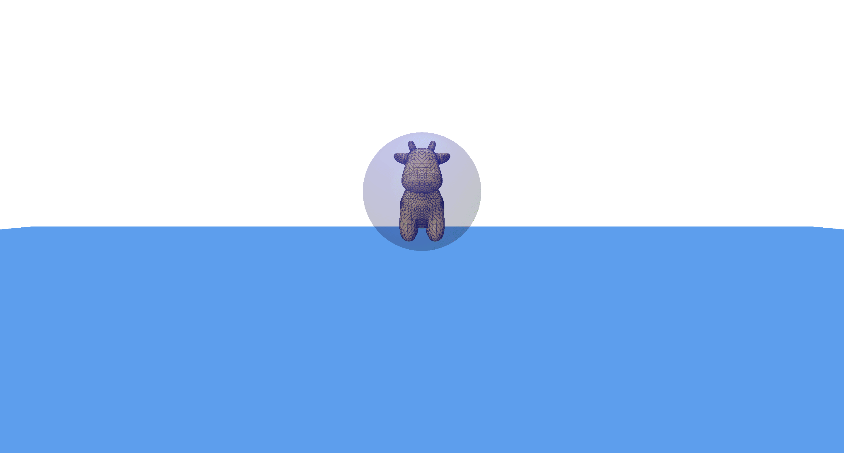
We start with a manifold triangular mesh e.g. Spot the cow, and tetrahedralize it using the python library of TetGen, a Delaunay-based tetrahedral mesh generator. [1] The resulting mesh is given as a \((V, C)\), where \(C\) is a set of tetrahedral cells whose vertices are in \(V\), as shown in Figure 1 below.
Figure 1: Tetrahedral mesh of Spot.
We use the Physics Based Animation Toolkit (PBAT) to compute the free vibrational modes of our model. Physically, one can describe vibration as the oscillatory motion of a physical structure, induced by energy exchanges of the potential (elastic deformation) and the kinetic (moving mass) energies. Vibrations are typically classified as either free or forced. In free vibrations, there are no continuous external forces acting on the structure, e.g. when a guitar string is plucked, while forced vibrations result from ongoing external forces. By looking at these free vibrations, we can determine the natural frequencies and normal modes of the structure.
First, we convert our geometricmesh into a FEM mesh and compute its Jacobian determinants and gradients of its shape function. You can check the documentation to learn more about FEM meshes.
Using these FEM quantities, we can model a hyperelastic material given its Young’s modulus \(Y\), Poisson’s ratio \(\nu\) and mass density \(\rho\).
rho = 1000.
Y = np.full(mesh.E.shape[1], 1e6)
nu = np.full(mesh.E.shape[1], 0.45)

# Compute mass matrix
M = pbat.fem.MassMatrix(mesh, detJeM, rho=rho, dims=3, quadrature_order=2).to_matrix()

# Define hyperelastic potential
hep = pbat.fem.HyperElasticPotential(mesh, detJeU, GNeU, Y, nu, energy=pbat.fem.HyperElasticEnergy.StableNeoHookean, quadrature_order=1)
Now we compute the Hessian matrix of the hyperelastic potential, and solve the generalized eigenvalue problem \(Av = \lambda M v\) using SciPy, where \(A\) denotes the Hessian matrix (a real symmetric matrix) and \(M\) denotes the mass matrix.
import scipy as sp

# Reshape matrix of vertices into a one-dimensional array
vs = mesh.X.reshape(mesh.X.shape[0]*mesh.X.shape[1], order="f")

hep.precompute_hessian_sparsity()
hep.compute_element_elasticity(vs)

HU = hep.hessian()
leigs, Veigs = sp.sparse.linalg.eigsh(HU, k=30, M=M, sigma=-1e-5, which="LM")
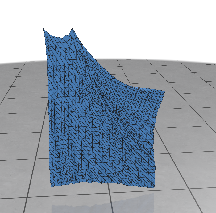
The resulting eigenvectors represent different deformation modes of the mesh. They can be animated as time continuous signals, as shown in Figure 2 below.
Figure 2: Six different deformation modes of Spot. Notice how each mode is characterized by deformations in a different local site of the mesh like its legs or neck.
Reduced Deformation Models
The BD-Tree paper [2] introduced the bounded deformation tree, which can perform collision detection for reduced deformable models at similar costs to standard algorithms for rigid bodies. But what do we mean exactly by reduced deformable models? First, unlike rigid bodies, where collisions affect only the position or movement of the object, deformable bodies can dynamically change their shape when forces are applied. Naturally, collision detection is simpler for rigid bodies than for deformable ones. Second, instead of explicitly tracking every individual triangle in a mesh, reduced deformable models represent complex deformations efficiently by a smaller set of parameters. This is achieved by using a linear superposition of pre-computed displacement fields that capture the essential ways a model can deform.
Suppose we have a triangular mesh with \(|V| = n\). Let \(\boldsymbol{p} \in \mathbb{R}^{3n}\) denote the undeformed vertices locations, and let \(U \in \mathbb{R}^{3n \times r}\) be a matrix with \(r \ll n\). Then the new deformed vertices location \(\boldsymbol{p’}\) are approximated by a linear superposition of \(r\) displacement fields given by the columns of \(U\) such that
where the amplitude of each displacement field is determined by the reduced coordinates \(\boldsymbol{q} \in \mathbb{R}^{r}\). Both \(U\) and \(\boldsymbol{q}\) must already be known in advance. In our case, the columns of \(U\) are the eigenvectors obtained from modal analysis described earlier, although they could also result from methods, e.g. an interpolation process. The reduced coordinates \(\boldsymbol{q}\) could also be determined by some possibly non-linear black box process. This is important to note: although the shape model is linear, the deformation process itself can be arbitrary!
Bounded deformation trees
Welzl’s algorithm
The BD-Tree works by constructing a hierarchy of minimum bounding spheres. As a first step, we need a method to construct the smallest enclosing sphere for some set of points. Fortunately, this problem has been well studied in the field of computational geometry, and we can use the randomized recursive algorithm of Welzl [3] that runs in expected linear time.
The Welzl’s algorithm is based on a simple observation: assume a minimum bounding sphere \(S\) has been computed a set of points \(P\). If a new point \(p\) is added to \(P\), then \(S\) needs to be recomputed only if \(p\) lies outside of \(S\), and the new point \(p\) must lie on the boundary of the new minimum bounding sphere for the points \(P \cup \{p\}\). So the algorithm keeps track of the set of input points and a set of support, which contains the points from the input set that must lie on the boundary of the minimum bounding sphere.
Sphere WelzlSphere(Point pt[], unsigned int numPts, Point sos[], unsigned int numSos)
{
	// if no input points, the recursion has bottomed out.
    // Now compute an exact sphere based on points in set of support (zero through four points)
	if (numPts == 0) {
		switch (numSos) {
			case 0: return Sphere();
			case 1: return Sphere(sos[0]);
			case 2: return Sphere(sos[0], sos[1]);
			case 3: return Sphere(sos[0], sos[1], sos[2]);
			case 4: return Sphere(sos[0], sos[1], sos[2], sos[3]);
		}
	}
	// Pick a point at "random" (here just the last point of the input set)
	int index = numPts - 1;
	// Recursively compute the smallest bounding sphere of the remaining points
	Sphere smallestSphere = WelzlSphere(pt, numPts - 1, sos, numSos);
	// If the selected point lies inside this sphere, it is indeed the smallest
	if(PointInsideSphere(pt[index], smallestSphere))
		return smallestSphere;
	// Otherwise, update set of support to additionally contain the new point
	sos[numSos] = pt[index];
	// Recursively compute the smallest sphere of remaining points with new s.o.s.
	return WelzlSphere(pt, numPts - 1, sos, numSos + 1);
}
The BD-Tree Method
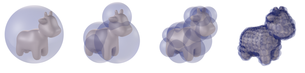
Figure 3: Wrapped BD-Tree for Spot at increasing recursion levels.
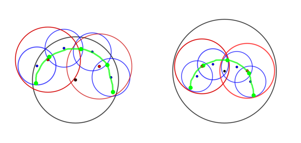
Now that we can compute the minimum bounding spheres for any set of points, we are ready to construct a hierarchical sphere tree on the undeformed model, after which it can be updated following deformation. First we note that the BD-Tree is a wrapped hierarchy, wherein the bounding spheres tightly enclose the underlying geometry but any bounding sphere at one level need not contain its child spheres. This is different from a layered hierarchy in which spheres must enclose their child spheres, but can fit the underlying geometry more loosely (see Figure 4).
Figure 4: An illustration—re-created from [2] of the wrapped hierarchy (left) and layered hierarchy (right). The underlying geometry is shown in green with five vertices and four edges.
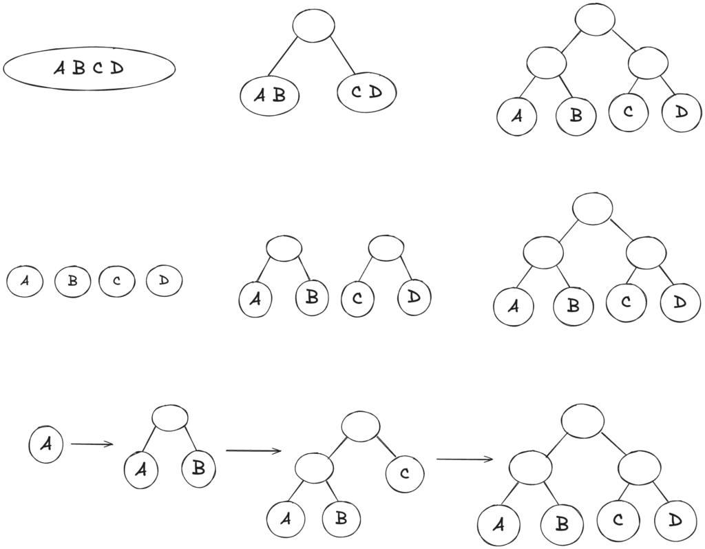
As shown in Figure 5, there are many possible approaches to building a binary tree. In our case, we use a simple top-down approach while partitioning the underlying geometry, i.e. we recursively split Spot at its median into two parts with respect to its local coordination axes, such that a leaf node (the lowest level) contains only one triangle.
Figure 5: Hierarchical binary tree construction with four objects using a top-down (top), bottom-up (middle) and insertion approach (bottom).
As the object deforms, how do we compute the new bounding spheres quickly and efficiently?
Let \(S\) denote a sphere in the hierarchical tree with center \(c\) and radius \(R\) containing the \(k\) points of the geometry \(\{p_{i}\}_{1 \leq i \leq k}\). After the deformation, the center of the sphere \(c\) is displaced by a weighted average of the contained points’ displacements \(u_{i}\) with weights \(\beta_i\) e.g. \(\beta_i := 1/k\) for \(1 \leq i \leq k\). So the new center can be expressed as
\(\displaystyle c’ = c + \sum_{i = 1}^{k} \beta_i u_i.\)
Using the displacement equation above, we can write \(u_i\) as the sum \(\sum_{j = 1}^{r} U_{ij} q_{j}\) and substitute this into the previous equation to obtain:
\(\displaystyle c’ = c + \sum_{j = 1}^{r} \left(\sum_{i = 1}^{k} \beta_i U_{ij}\right) q_j = c + \bar{U} \boldsymbol{q}.\)
To compute the new radius \(R’\), we make use of the triangle inequality
Thus, we have an updated bounding sphere \(S’\) with its center \(c’\) and radius \(R’\) computed as functions of the reduced coordinates \(\boldsymbol{q}\).
Figure 6: Spot colliding with ground plane. The colors of the spheres change based on the ratio of \(R\) in the undeformed state to \(R’\) in the deformed state.
References
[1] Hang Si. TetGen, a Delaunay-based quality tetrahedral mesh generator. ACM Transactions on Mathematical Software, 41(2), 2015.
[2] Doug L. James and Dinesh K. Pai. BD-Tree: Output-Sensitive Collision Detection for Reduced Deformable Models. ACM Transactions on Graphics, 23(3), 2004.
[3] Emo Welzl. Smallest enclosing disks (balls and ellipsoids). New Results and New Trends in Computer Science, 555, 1991.
[4] Christer Ericson. Real-Time Collision Detection. CRC Press, Taylor & Francis Group. Chapter 4, p. 99-100. 2005.
Project Mentor: Justin Solomon (MIT, USA) Volunteers: Biruk Ambaw (Université Paris-Saclay, Fr), Andrew Rodriguez (Georgia Institute of Technology, USA), and Josh Vekhter ( UT Austin, USA)
Acknowledgments. Sincere thanks to Professor Justin Solomon for his invaluable guidance throughout this project. His carefully designed questions and coding tasks not only deepened my understanding of core topics in geometry processing in a short amount of time, but also sharpened my coding skills—and ensured my lunch breaks were notably shorter than they might have been otherwise :). I would also like to thank Josh Vekhter, Andrew, and Biruk for their support and valuable feedback to my teammates and me. In addition to the math and codes, Professor Justin and Josh taught me the value of a well-timed joke to lighten the load!
Introduction
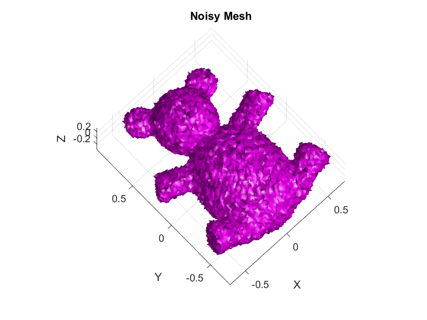
Mean Curvature Flow (MCF) is a fundamental geometric evolution partial differential equation (PDE) that describes the motion of a surface \(\mathcal{M}_t \subset \mathbb{R}^3\) under its mean curvature. Each point on the surface moves in the direction of the unit normal vector to the surface with velocity proportional to the mean curvature, leading to a smoothing effect that regularizes the geometry of the surface over time. MCF is widely studied in differential geometry and geometric analysis due to its intrinsic connection to minimal surfaces and its role in shape optimization. In computational applications, MCF is particularly useful in geometry processing (GP), including tasks such as surface fairing, mesh denoising, and feature-preserving smoothing.
The discretization of the MCF PDE consists of both spatial and temporal components. Spatial discretization is well-established, with common techniques such as finite element methods, discrete exterior calculus, and discrete differential geometry effectively approximating the part of the equation that governs the surface’s spatial evolution. In contrast, temporal discretization remains challenging due to stability constraints and accuracy limitations.
Three primary approaches exist for temporal discretization: explicit, implicit, and semi-implicit methods. Explicit methods, like forward Euler, often become unstable with larger time steps. Implicit methods, such as backward Euler, offer stability but at a high computational cost. Semi-implicit methods, like the one introduced by Desbrun et al. (1999), strike a compromise between these two extremes but may still fall short in terms of accuracy and stability. In practice, the temporal discretizations that are commonly employed in the literature are only first-order accurate thus, may not provide the desired level of accuracy and stability we ideally wish for.
The central focus of this project was to derive and implement higher-order temporal discretizations—both explicit and semi-implicit—for MCF on triangular meshes, with the goal to improve the numerical accuracy of the discrete evolution of the surface by reducing truncation errors and better approximating the continuous PDE solution, particularly for larger time steps. By increasing temporal accuracy, we aim to enhance both the fidelity of the simulated flow and the computational efficiency, mitigating the need for excessively small time steps while maintaining stability.
In this article, I externalize my internal exploratory journey and insights gained during my last SGI research week under the guidance of my mentors. The article begins with an introduction to MCF and its significance in GP, followed by a brief discussion on the process of discretization followed by the derivation of spatial discretization via finite element methods and first-order accurate temporal discretization via finite difference methods for MCF. A theoretical comparison of the methods in question is then provided, highlighting their pros and cons. Finally, we derive the second-order accurate temporal discretization of MCF, in both, the explicit, and semi-implicit schemes. Empirical validations of theoretical results are also presented, along with a humorous fail. The goal here is on exposition, rather than taking the shortest path.
Understanding Mean Curvature Flow in \(\mathbb{R}^3 \)
Formal Definition
Let \(M_t \subset \mathbb{R}^3\) represent a family of smoothly embedded surfaces parameterized by time \(t\). The surface at time \(t\) can be described by a smooth mapping:
\(U\) is an open set in \(\mathbb{R}^2\) representing the parameter space of the surface, with local coordinates \( \mathbf{u} = (u_1, u_2)\).
\([0,T) \) represents time, where \(T\) is the time until which the flow is considered.
\(X(\mathbf{u}, t)\) is the position vector of a point on the surface in \(\mathbb{R}^3\) at time \(t\), and can be explicitly written as: \[ X(\mathbf{u},t) = \begin{pmatrix} X_1(\mathbf{u},t) \\ X_2(\mathbf{u},t) \\ X_3(\mathbf{u},t) \end{pmatrix} \] and \(X_1(\mathbf{u},t), X_2(\mathbf{u},t), X_3(\mathbf{u},t)\) are the coordinate functions that determine the \(x, y,\) and \(z\) components of the position vector in \( \mathbb{R}^3\)
The mean curvature flow is then dictated by the following partial differential equation:
\(\frac{\partial X}{\partial t}(\mathbf{u}, t)\) is the velocity of the surface at the point \(X(\mathbf{u}, t)\).
\(H(\mathbf{u}, t)\) is the mean curvature at the point \(X(\mathbf{u}, t)\).
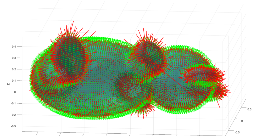
\(\mathbf{n}(\mathbf{u}, t)\) is the unit normal vector at the point \(X(\mathbf{u}, t)\), pointing outward or inward. It indicates the direction in which the surface will move during the flow.
\( \Delta \) is the Laplace-Beltrami operator associated with the surface \(M_t\).
Abuse of Notation. For simplicity, any operator \( \phi (\mathbf{u},t) \) at a point parameterized by \( (\mathbf{u},t))\) will be referred to simply as \( \phi \) in this article. The Laplace-Beltrami operator, might sometimes be referred to as the Laplacian depending on my mood.
Mean Curvature \(H\):
The mean curvature \( H\) at a point is defined as the average of the principal curvatures \( k_1 \) and \( k_2 \) at that point on the surface: \[ H= \frac{1}{2} (k_1 + k_2) \]
Where \(k_1\) and \(k_2\) are the eigenvalues of the second fundamental form of the surface. These principal curvatures measure the maximum and minimum bending of the surface in orthogonal directions at this particular point in question.
Alternative Expressions for \( H \):
Divergence of the Normal Vector Field: \(H\) can be expressed as the negative half of the divergence of the unit normal vector field \(\mathbf{n}\) on the surface: \( H= – \frac{1}{2} div ((\mathbf{n})) \).
Trace of the Shape Operator: In addition, \(H\) can be written as the trace of the shape operator (or Weingarten map) associated with the surface. This representation connects the mean curvature to the linear transformation that describes how the surface bends.
Why Study MCF?
Understanding MCF begins with a simple question: what happens when a surface evolves according to its own curvature? In practice, this flow helps smooth surfaces over time, driving them toward more regular shapes. This process is especially intriguing because it captures essential properties of geometric evolution without external forces, relying solely on the surface’s own shape.
A fundamental result by Huisken in 1984 in his paper titled “Flow by Mean Curvature of Convex Surfaces into Spheres” provides deep insight into this phenomenon. Huisken studied the evolution of a special type of hypersurfaces under MCF, and proved that any strictly convex smooth hypersurface, under MCF, evolves into a sphere before collapsing to a point in a finite, self-similar manner in a finite time. His work highlights how MCF transforms surfaces, regularizing their shape as they shrink and demonstrating the flow’s inherent tendency to round out irregularities. In mathematics, it is common practice to first test an idea or prove a theorem in simple and nice settings (such as convex compact spaces) before attempting to test/generalize to more abstract spaces.
While the general theory of MCF applies to a wide range of surfaces, it is particularly insightful to consider how a sphere—a familiar, symmetric object—shrinks under the flow. The sphere offers a clean, intuitive example where the underlying mathematics remains manageable, yet it showcases the essential features of MCF, such as shrinking to a point while maintaining symmetry. This serves as an ideal starting point for understanding more complex behaviors in less regular surfaces, grounded in the theoretical framework established by Huisken’s work.
Example: Shrinking Sphere Under MCF
Consider a sphere of radius \(R(t)\) at time \(t\). Under MCF, the sphere’s surface shrinks over time. We want to find how the volume of the sphere changes as it evolves under this flow.
For a sphere of radius \(R(t)\), the mean curvature \(H\) is given by: \( H=\frac{2}{R(t)}\), and the normal vector \(\mathbf{n}\) points radially inward, so: \(\mathbf{n}=\frac{−X}{R(t)}\)
Substituting these in the MCF equation: \( \frac{\partial X}{\partial t}=\frac{-2}{R(t)} \frac{-X}{R(t)}=\frac{2X}{R^2(t)}\)
To determine how the radius \(R(t)\) changes over time, observe that each point on the surface \(X\) can be written as: \(X=R(t) \mathbf{u}\) where \(\mathbf{u}\) is a unit vector in the direction of \(X\). Thus, \( \frac{\partial X}{\partial t} = \frac{\partial (R(t) \mathbf{u})}{\partial t} = \frac{2\mathbf{u}}{R(t)} \), which simplifies to \( \mathbf{u}\frac{dR(t)}{dt}= \frac{2 \mathbf{u}}{R(t)}\) so \(\frac{dR(t)}{dt}= \frac{2 }{R(t)} \).
To solve for \( R(t) \), we separate the variables and integrate \(\int R(t) \, dR(t) = \int 2 \, dt \) which gives \(\frac{R^2(t)}{2} = 2t + C \), where \( C \) is the constant of integration. Solving for \( R(t) \) gives \( R(t) = \sqrt{4t + C’} \) where \( C’ = 2C \). If we consider the initial condition \( R(0) = R_0 \), then \( R_0^2 = C’ \), and hence: \(R(t) = \sqrt{R_0^2 – 4t} \)
Volume Shrinkage:
The volume \( V(t) \) of the sphere at time \( t \) is \( V(t) = \frac{4}{3} \pi R^3(t) \). As the sphere shrinks over time, the volume decreases according to the following equation: \( V(t) = \frac{4}{3} \pi \left(R_0^2 – 4t \right)^{3/2} \), and it continues to shrink until \( t = \frac{R_0^2}{4} \), at which point the radius reaches zero and the sphere vanishes.
The accompanying animation illustrates the shrinking process, showing how both the radius and volume decrease over time under the influence of MCF until the sphere vanishes. The MCF drives the surface points of the sphere inward in the direction of the inward normals, leading to a uniform shrinking process. For a perfectly symmetric object like a sphere, the shrinking occurs uniformly, preserving the spherical shape until the radius reduces to zero.
The shrinking radius is computed via the derived formula above, \( R(t)= \sqrt{R_0^2 – 4t} \), and the shrinking becomes faster as time progress. The plots that are displayed at the end show the relation between \( R(t) \) and \( V(t) \) over time.
Shrinking sphere under MCF + evolution over time plots
Since computer machines operate in a discrete, digital environment, and GP is inherently computational, continuous geometric surfaces must be represented in a form that computer machines can process. This form is typically a mesh, a discrete approximation of a surface composed of vertices, edges, and faces, and given that MCF is intrinsically a continuous model described by a PDE in space and time, directly applying it to meshes necessitates the discretization of its continuous operators (the Laplacian and time derivatives) as well.
Discretizing MCF
As implied by the above paragraph, discretization is the process of transforming a continuous mathematical model \(\mathcal{M}\), which is defined over a continuous domain \(\Omega \subset \mathbb{R}^n\) and governed by continuous variables \(u(x)\) and operators \(\mathcal{L}\), into a discrete model \(\mathcal{M}_h\) suitable for computational analysis. This involves:
Replacing the continuous domain \(\Omega\) with a finite set of discrete points or elements \(\Omega_h = {x_i}_{i=1}^N\).
Approximating continuous functions \(u(x)\) by discrete counterparts \(u_h(x_i)\).
Substituting continuous operators \(\mathcal{L}\) with discrete analogs \(\mathcal{L}_h\).
The goal is to ensure that the discrete model \(\mathcal{M}_h\) preserves key properties such as consistency, stability, and convergence, so that \(\mathcal{M}_h\) faithfully reflects the behavior of the continuous model \(\mathcal{M}\) as the discretization is refined, i.e., as \(h \rightarrow 0\).
While many continuous models can be discretized, the accuracy and efficiency of the approximation depend on the chosen discretization technique and its implementation. Common discretization techniques include: Finite difference methods (FDM), finite element methods (FEM), finite volume methods (FVM), and spectral methods.
Discretizing the MCF model can be systematically divided into two main components: spatial discretization and temporal discretization. In this article, we employ the FEM for spatial discretization and the FDM for temporal discretization.
Spatial Discretization via FEM
Spatial discretization involves representing the continuous spatial domain of the model as a mesh and approximating differential operators—primarily the Laplacian, and also gradient and divergence as quantities at the discrete mesh in question.
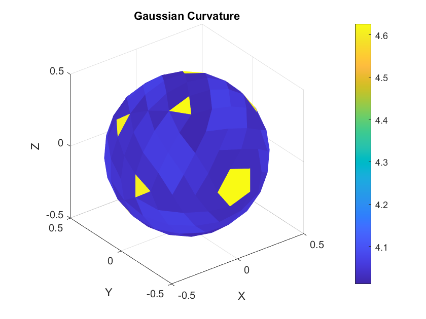
Assume the surface in question is discretized into a mesh which consists of a collection of triangular elements \(\{T_i\}\) with vertices \(v_j\). The first step to approximate the Laplace-Beltrami operator is to define basis functions \(\{\phi_j\}\) associated with the vertices and defined over \(T_i\). These are often linear or piecewise linear functions, \(\phi_j\) takes the value 1 at vertex \(v_j\) and 0 at all other vertices. These basis functions form a set that allows any function \(X\) on the surface to be approximated as a linear combination of them \( X≈ \sum_j X_j \phi_j\), where \(\mathbf{X_j}=\mathbf{X(v_j)}\) represents the value of the position function at vertex \(v_j\).
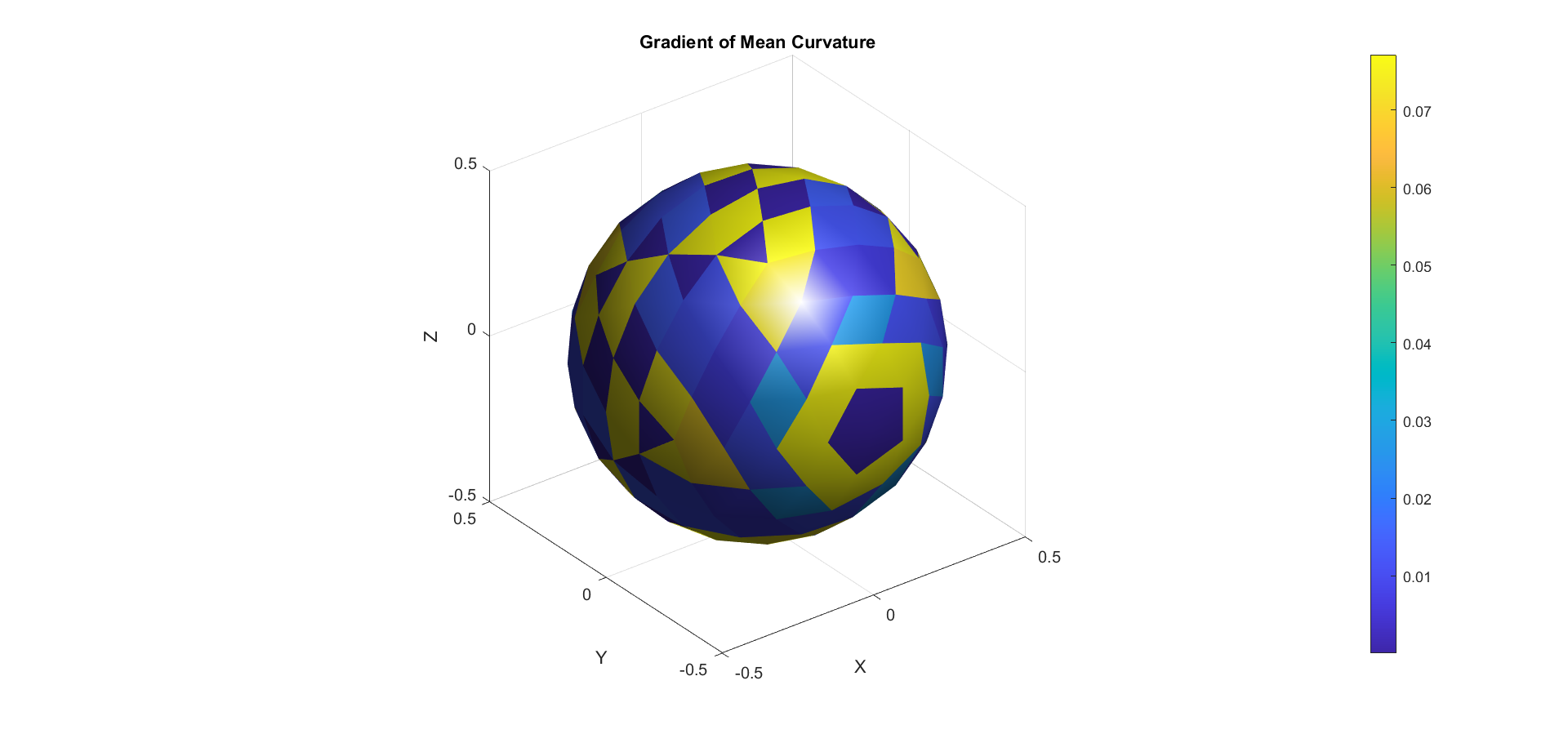
Next, we compute the gradient of each basis function within each triangle, which will be constant over the triangle because the functions are linear. The Laplacian operator, which in continuous terms is the divergence of the gradient, is discretized by integrating the product of the gradients of the basis functions over the surface. This leads to the construction of the stiffness matrix \(\mathbf{L}\), where each entry \( \mathbf{L_{ij}}\) is derived from the inner products of the gradients of the basis functions \(\phi_i\) and \(\phi_j\) ( \( \nabla \phi_i\) and \(\nabla \phi_j\)), weighted by the cotangent of the angles opposite the edge connecting vertices \(v_i\), and \(v_j\). The diagonal entries \(\mathbf{L_{ii}}\) sum the contributions from all adjacent vertices.
More precisely, for two vertices \(v_i\) and \(v_j\) connected by an edge, the stiffness matrix \(\mathbf{L}\) is computed using the following integral:
\[ \mathbf{L_{ij}}=\int_{\sigma} \nabla \phi_i \cdot \nabla \phi_j dA\] where \(\sigma\) is the surface, and \(dA\) is the area element.
For a piecewise linear basis function on a triangular mesh, those gradients in question are constant within each triangle, so the integral simplifies to the sum over the triangles \(T_k\) that include the edge connecting \(v_i\) and \(v_j\):
Where \( N(v_i,v_j)\) denotes the set of triangles sharing the edge between \(v_i\) and \(v_j\). Now the inner product \(\nabla \phi_i \cdot \nabla \phi_j\) can be computed using the cotangent formula \[\nabla \phi_i \cdot \nabla \phi_j = \frac{-1}{2 \text{Area}(T_k)}(\cot{\alpha_{ij}}+\cot{\beta_{ij}}) \]
Finally the diangonal enteries \(\mathbf{L_{ii}}\) sum the contributions from all the adjacent verticies: \[\mathbf{L_{ii}}=\sum_{i \neq j} \mathbf{L_{ij}} = \sum_{i \neq j} \frac{1}{2} (\cot{\alpha_{ij}}+\cot{\beta_{ij}})\]
To balance the discretization, we also need the mass matrix \(\mathbf{M}\), which arises from integrating the basis functions themselves. Formally, the entries of the mass matrix \(\mathbf{M}\) are given by: \[ \mathbf{M_{ij}} = \int_{\sigma} \phi_i \phi_j dA\]
In simple cases1, the mass matrix is typically diagonal, with each entry written as: \[ \mathbf{M}_{ii} = \frac{1}{3} \sum_{T \ni v_i} \text{Area}(T),\]
where the sum is over all triangles \(T\) that share the vertex \((v_i).\) The final discretized Laplace-Beltrami operator is represented by the generalized eigenvalue problem \(\mathbf{L}X = \lambda \mathbf{M} X\), where \(\mathbf{L}\) encodes the differential operator and \( \mathbf{M}\) ensures that the discretization respects the geometry of the mesh.
Both matrices (the mass matrix \( \mathbf{M}\) and the stiffness matrix \( \mathbf{L}\)) are positive semi-definite, and sparse.
Intuitively,
The stiffness matrix \(\mathbf{L}\) captures the geometric and differential properties of the surface. It represents how the curvature is distributed over the mesh by measuring how the gradients of the basis functions (associated with each vertex) interact with each other. The entries of this matrix are weighted by the angles in the triangles, which essentially encode how “stiff” or “resistant” the mesh is to deformation. In other words, it determines how much the shape of the surface resists change when forces (like curvature flow) are applied.
The mass matrix \(\mathbf{M}\) accounts for the distribution of area or “mass” over the surface. It ensures that the discretization respects the surface’s geometry by distributing weight across the vertices according to the areas of the surrounding triangles. This matrix is often diagonal, with each entry corresponding to the area associated with a vertex, making sure that the mesh’s physical properties, like area and volume, are properly balanced in computations.
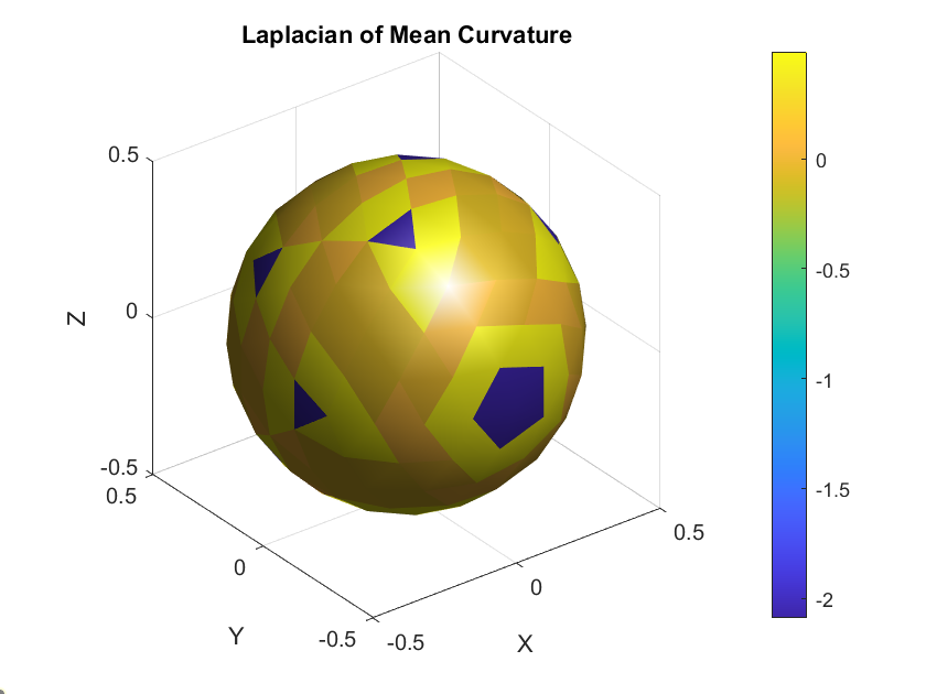
Solving the general eignvalue problem, we reach the following approximation of the Laplacian: \(\Delta \approx \mathbf{M}^{-1} \mathbf{L}\).
Remark: In discretizing the Laplacian operator, several other approaches can be employed too such as divided difference, higher-order elements, discrete exterior calculus,..etc. In any case, no discretization approach of the Laplacian could keep every natural property of its ideal continuous form.
Temporal Discretization via FDM
Temporal discretization refers to the approximation of the time-dependent aspects of the MCF model (the time derivative \(\frac{\partial X}{\partial t}\)). This step is critical for evolving the surface over time according to the mean curvature dynamics. Three common approaches are used for this type of discretization: Explicit methods (e.g. Explicit Euler method), Implicit methods (e.g. Implicit Euler method), and Semi-implicit methods (e.g Desbrun et al. (1999)).
Explicit Euler Method: This method (also known as forward Euler method) is where the new future positions of the mesh vertices are computed based on the current positions and the mean curvature at those positions. While this method is simple to implement, it may impose stability constraints on the time step size. The discretized vertex update rule is given by: \[\frac{X^{(k+1)} – X^{(k)}}{\Delta t} = \mathbf{M}^{-1} \mathbf{L} X^{(k)} \] Rearranging this, we get: \[ X^{(k+1)} = X^{(k)} + \Delta t \mathbf{M}^{-1}\mathbf{L} X^{(k)} \] where \(X^{(k)}\) and \(X^{(k+1)}\) are surface position matrix of the mesh vertices at time steps \(k\) and \(k+1\), respectively.
Implicit Euler Method: Also known as backward Euler, this method involves solving a system of equations at each time step, it might provide greater stability compared to the Explicit Euler method and allow for larger time steps. The discretized vertex update rule is given by: \[ X^{(k+1)} \approx X^{(k)} + \Delta t \mathbf{M}^{-1}\mathbf{L} X^{(k+1)} \] This equation is said to be fully implicit because the Laplacian depends on the vertex positions at the time step one is trying to solve for, making it nonlinear and difficult to solve.
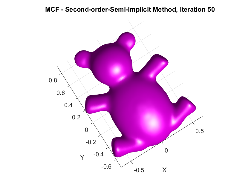
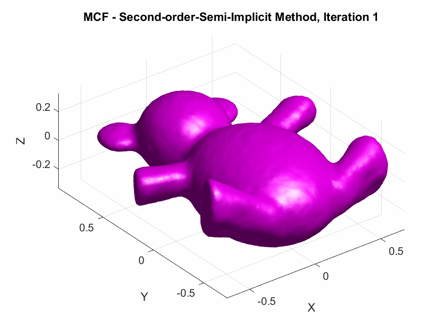
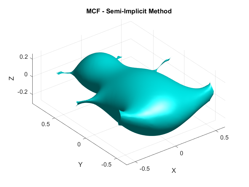
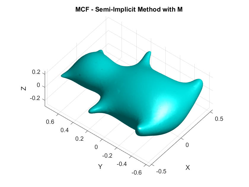
Desbrun et al.’s Semi-Implicit Method: (Desbrun et al. 1999) proposed a semi-implicit method, which is a compromise between the simplicity of explicit methods and the stability of implicit methods. The idea is to treat the Laplacian and the vertex positions in the following manner: Instead of calculating the Laplacian at the next time step (which makes the equation nonlinear), they compute it at the current time step which simplifies the problem, and the vertex positions are still updated at the next time step. Their discretized vertex update rule is given by: \[ X^{(k+1)} \approx X^{(k)} + \Delta t\mathbf{M^{-1}}(\mathbf{L}X^{(k)} )X^{(k+1)} \] This equation is still implicit in \(X^{(k+1)}\), but the Laplacian is evaluated at the known positions \(X^{(k)}\), making the system linear and easier to solve. The update rule can be re-arranged into: \[X^{(k+1)} \approx (I- \Delta t\mathbf{M^{-1}L}X^{(k)} )^{-1}X^{(k)} \]. This method offers nice stability. However, it is not as accurate as fully implicit methods, because it only approximates the Laplacian based on the current positions. It might smooth the mesh, but not as precisely as solving the full nonlinear system such as the fully-implicit. In addition, it does not generalize to other geometric flows that require more complex handling of nonlinearities.
Adaptive Time Stepping: This approach adjusts the time step size dynamically based on the evolution of the surface, allowing for finer resolution during critical changes and coarser resolution during smoother phases. Progyan Das from my team worked on this approach.
Remark. The derivations for the above update rules are tacitly included in the part we derive their second-order forms.
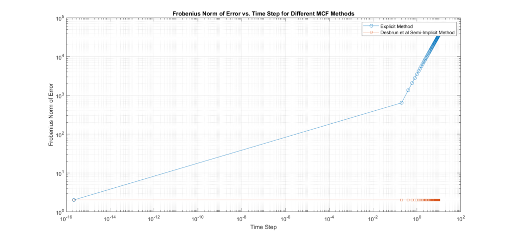
Comparative Analysis and Empirical Validation: Euler Explicit vs. Desbrun et al.’s
Accuracy
Euler Explicit Method:
Order of Accuracy: This method is first-order accurate in time, meaning that the global error in the solution decreases linearly with the time step \(\Delta t\). If the exact solution at time \(t\) is denoted by \(X_{t}\) and the numerical solution by at time \(t_n\) by \(X_{t_n}\), the error \(E_n = X(t_n) \) satisfies\(E_n \approx C \Delta t\), where \(C\) is a constant dependent on the problem. This linear relationship implies that halving the time step approximately halves the error.
Error Propagation: Errors tend to accumulate more rapidly, especially for larger time steps. Because this method updates the solution based only on information from the current time step so, if the time step \(\Delta t\) is too large, the method may not accurately capture the evolution of the curvature, leading to significant errors that compound over time. The error propagation can be expressed as \(X^{(k+1)}=X^{(k)}+ \Delta t \dot F(X^{(k)})\), where \(F(X^{(k)})\) is the update function. If\(\Delta t\) is too large, the local truncation error, which is \(O(\Delta t^2)\), becomes significant, causing larger cumulative errors.
Handling of Complex Geometries: Will probably struggle with highly irregular meshes, which is a direct consequence of the above bullet. leading to larger errors in curvature computation.
Desbrun et al. Semi-Implicit Method:
Order of Accuracy: This method is also first-order accurate in time because it is essentially a modified backward Euler scheme, where the implicit part is handled for spatial discretization, but the time discretization remains first-order.
Error Propagation Reduction: The method implicitly handles the curvature of the mesh by solving a linear system at every update, which incorporates more information about the solution at the next time step. This implicit approach effectively reduces errors, and stabilizes the solution especially when larger time steps are used compared to Euler’s explicit method.
Numerical Diffusion: Moreover, it has a better control over numerical diffusion —a phenomenon where fine details of the mesh are smoothed out excessively—compared to the explicit method, leading to more accurate smoothing. Numerical diffusion can be mathematically described by how the curvature smoothing term affects the higher-order modes of the solution and here is where the implicit nature of the method helps preserve these modes more effectively than Euler’s explicit method.
Stability
Euler Explicit Method:
Conditionally Stable: The stability here depends on the time step size; it requires small time steps to maintain stability.
CFL Condition: The time step must satisfy the Courant-Friedrichs-Lewy (CFL) condition, which can severely restrict the time step size, especially for fine meshes. The CFL condition constrains the time step to be inversely proportional to the square of the mesh resolution. This means that as the mesh becomes finer, the time step must decrease quadratically, which significantly increases the number of iterations required for convergence.
Desbrun et al. Semi-Implicit Method:
Unconditionally Stable: Allows larger time steps without sacrificing stability. This is a key advantage for computational efficiency.
Robustness: More stable under large deformations or irregular meshes, making it suitable for a broader range of applications than the explicit method.
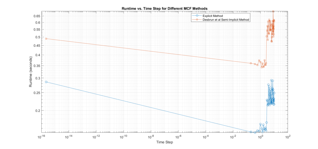
Computational Efficiency and Memory Usage
Euler Explicit Method:
Efficiency: Simpler to implement and faster per iteration due to direct updates, but requires more iterations for convergence due to the small time steps needed.
Memory Usage: Lower memory requirements since it does not require solving linear systems.
Parallelization: Easier to parallelize due to the independence of the update steps.
Desbrun et al. Semi-Implicit Method:
Efficiency: More computationally intensive per iteration due to the need to solve linear systems, but fewer iterations may be needed due to larger permissible time steps.
Memory Usage: Higher memory consumption due to the storage of matrices for linear system solving.
Parallelization: More challenging to parallelize because of the dependencies introduced by solving the linear system.
Implementation Complexity
Euler Explicit Method:
Complexity: Conceptually simpler and easier to implement. It involves straightforward updates without the need for solving linear systems.
Dependencies: Minimal dependencies between updates, making it a more accessible method for quick implementations.
Desbrun et al. Semi-Implicit Method:
Complexity: More complex to implement due to the need to solve large, sparse linear systems at each time step.
Dependencies: Involves matrix assembly and inversion, which can introduce additional challenges in implementation.
Parameter Sensitivity
Euler Explicit Method:
Sensitivity: Highly sensitive to time step size. Small changes can significantly affect stability and accuracy.
Desbrun et al. Semi-Implicit Method:
Sensitivity: Less sensitive to time step size, allowing for greater flexibility in choosing time steps.
Overall Assessment:
Euler Explicit Method is advantageous for its simplicity, ease of implementation, and parallelization potential. However, it is limited by stability constraints, accuracy issues, and higher sensitivity to parameter choices.
Desbrun et al. Semi-Implicit Method offers superior stability, accuracy when compared to the explicit, and reduced numerical diffusion at the cost of increased computational complexity and memory usage. It is better suited for applications requiring robust and accurate smoothing, particularly in the context of complex or irregular meshes.
Oh… this felt like eating five horrible McDonald’s cheeseburgers. 🍔🍔🍔🍔🍔 Right? So, let’s compress this previous analysis into a nice compact table for quick reference.
Aspect
Euler Explicit Method
Desbrun et al. Semi-Implicit Method
Accuracy
First-order accurate in time. Higher error accumulation, especially for large time steps. Struggles with complex geometries.
First-order accurate in time. Better error reduction, especially for large time steps. Better control over numerical diffusion.
Stability
Conditionally stable. Requires small time steps, dictated by the CFL condition.
Unconditionally stable. Allows larger time steps without sacrificing stability.
Computational Efficiency
Simple and fast per iteration. Inefficient for fine meshes due to small time step requirement.
Computationally more expensive due to solving linear systems. Efficient for larger time steps.
Memory Usage
Lower memory usage.
Higher memory usage due to storing and solving linear systems.
Implementation Complexity
Relatively simple to implement.
More complex due to the need to solve linear systems.
Parallelization
Easier to parallelize due to independent updates.
More challenging to parallelize due to solving linear systems.
Parameter Sensitivity
Sensitive to time step size (CFL condition).
Less sensitive to time step size, allowing more flexibility.
Numerical Diffusion
Higher numerical diffusion, especially for large time steps.
Better control over numerical diffusion, preserving more detail.
Euler explicit vs Desbrun et al. semi-implicit methods compact comparative assessment
The next experiment aims to empirically illustrate the above tradeoffs in the stability and accuracy aspects presented above for the two methods in question for MCF since the main aim of the project is to come up with an approach to improving the accuracy and stability of MCF applied to triangle meshes by incorporating higher-order derivatives in the time integration process.
Experimental Design:
Mesh Preparation:
Target Mesh: Load a 3D mesh model, and store it as the target mesh.
Noisy Mesh: Add a controlled amount of noise to simulate imperfections to the target mesh and store the output as the noisy mesh.
Application of MCF Methods:
Apply each MCF method to the noisy mesh across a series of pre-determined range of time steps. The number of iterations for both methods is fixed (10 iterations) per each time step. Choose the range of the time steps such that it includes very small (those satisfying the CFL condition) to relatively large time steps to allow for a comprehensive analysis of the methods’ behavior under different conditions.
Data Logging: For each time step, record the following data for each method:
Error Metric: Frobenius norm of the difference between the smoothed mesh and the original target mesh.
Stability Metric: the number of maximum \(\Delta t\) where the error stays less than a pre-determined error threshold by the user.
Computational Time: Time taken for execution.
Output Plots
Error vs. Time Steps: The error is plotted against the time step size on a log-log scale. The slope of this curve will indicate the convergence rate:
Steeper Slope: Indicates faster convergence and higher accuracy.
Flatter Slope: Suggests slower convergence and potential inaccuracies.
Visual and Quantitative Evaluation: The final smoothed meshes are presented for visual comparison against the target mesh.
Time Step Limitations: The maximum time step for which each method remains stable is identified.
Frobenius norm vs time steps size for Euler’s explicit and Desbrun et al.’s semi-implicit methodsRuntime (seconds) vs time steps size for Euler’s explicit and Desbrun et al.’s semi-implicit methods
Interpretation of Results:
The accuracy plot shows that the Explicit method tends to produce much higher errors compared to the Desbrun’s especially at larger time steps, confirming that it requires small time steps to maintain stability. In addition, we can see that with Desbrun’s, the error remains constant across a wide range of varying time steps, this confirms that the method’s accuracy and stability are not affected by the choice of time step within the range tested, it also verifies its robustness, and tendency to reduce error propagation as time step sizes increase. In regards to the rate of convergence, the slope of the error curve vs time-steps in Euler’s explicit is \(m=1.29\), and Desbrun’s method rate of convergence is \(m=1\).
In this experiment, we set the error threshold to 3. Turns out the maximum step size \(\Delta t\) where the error is below this threshold for Euler’s explicit is 2.2204e-16 while for Desbrun et al.’s is (the final in our range).
Inspiration: This experimental design was inspired by a task I did during my second SGI project on 2D Differentiable Representation of Curve Networks, under Mikhail Bessmeltsev. 🙂
The Case for Higher-Order Time Discretization
As demonstrated by both theory and practice, even robust methods like Desbrun et al.’s semi-implicit method for MCF face limitations with first-order time discretization. While this category of methods offers a compromise between explicit and fully implicit methods, first-order discretization still imposes constraints on accuracy in numerical simulations. These limitations stem from the truncation errors inherent in first-order approximations.
First-order methods approximate the time derivative using only vertex velocities (the first derivative of position with respect to time) and disregard higher-order terms, such as acceleration (the second derivative). This omission means they fail to account for how the geometry of the surface might be changing or accelerating locally since higher derivatives encode information about local curvatures. If we conceptualize the next iterate as\(X^{(k+1)}_i = \mu (X_i^{(k)}, I^{(k)})\) where \(I^{(k)}\) is an information vector, local geometric properties of the surface at the current iterate \(X_i^{(k)}\), it becomes clear that the more detailed information we incorporate into \(I^{(k)}\), the more accurate the next state \(X^{(k+1)}_i \) will be.
In other words, higher-order discretizations, such as second-order ones, lead to a significant reduction in truncation errors, better convergence, and a more accurate representation of the geometry over time for larger time steps which contributes to a more economical utilization of computational resources (e.g reduced number of iterations).
Deriving Higher-order Discretizations for MCF
In this section, we derive the second-order accurate, in time, vertex update rules for the explicit forward Euler and the semi-implicit due to Desbrun et al. Starting from the continuous form of the MCF equation, we use a Taylor expansion to approximate the position of a point on the surface up to the second-order term, and for Desbrun et al.’s, we make use of Neumann series in our derivation.
Recall that from the first section, the MCF in its continuous form, is described following equation:
where: \( X(u,t) \in \mathbb{R}^3 \) is the position of a point on the surface at parameter \( u \) and time \( t \), and \(\Delta\) is the Laplace Beltrami operator.
Now, we apply a Taylor expansion of \( X(u,t) \) around time \( t=t_k\):
Where, \[\frac{\partial^2 X(u,t)}{\partial t^2}\Bigg |_{t=t_k} = \frac{\partial}{\partial t} \left( \Delta X(u,t) \right) \Bigg |_{t=t_k}\] This follows from the definition of Laplace Beltrami operator and Schwarz’s Theorem (also known as Clairaut’s Theorem on Equality of Mixed Partials)
Now let \( X^{(k)}_i\), \( X^{(k+1)}_i \) denote the position vector of vertex \(i\) at times \( t_k \), and\( t_{k+1} \) respectively, and \( \Delta t = t_{k+1}-t_k\). Using the Taylor expansion in \((*)\), the second-order vertex update rule becomes:
Now the spatial discrete approximation we use in this article is \(\Delta \approx \mathbf{ML}^{-1}\). Now we can write the vertex update rule for Forward Euler as follows: \[ X^{(k+1)}_i\approx X^{(k)}_i + \Delta t \mathbf{ML}^{-1} X^{(k)}_i + \frac{\Delta t^2}{2} (\mathbf{ML}^{-1})^2 X^{(k)}_i \]
After doing some algebra, we reach the following matrix form:
\[ X^{(k+1)} \approx [ I + \Delta t \mathbf{ML}^{-1} + \frac{\Delta t^2}{2} (\mathbf{ML}^{-1})^2] X^{(k)} \]
For the semi-implicit form due to Desbrun et al.’s, things are a bit tricky. It should be easy by now to derive the first-order vertex update presented earlier in (ref) using Taylor expansion which takes the matrix form:
To derive the second order term for this scheme, we expand the inverse matrix \( \left(I – \Delta t \mathbf{M}^{-1} L X^{(k)} \right)^{-1} \) using a Neumann series, but for this to work, we have to ensure that \( \mathbf{M}^{-1}L X^{(k)}\) satisfies the condition for convergence, i.e., its spectral radius is strictly less than 1: \[ \rho (\Delta t \mathbf{M}^{-1}L X^{(k)} )<1 \]
This means \(\Delta t\) must be chosen small enough, or the structure of \(\mathbf{M}^{-1}L X^{(k)}\) must ensure that its eigenvalues are small.
Assuming this is true, the Neumann series expansion for \( \left(I – \Delta t \mathbf{M}^{-1}L X^{(k)} \right)^{-1} \) can be written as: \[ \left(I – \Delta t \mathbf{M}^{-1} L X^{(k)}\right)^{-1} = I + \Delta t \mathbf{M}^{-1} L X^{(k)}+ \Delta t^2 \left(\mathbf{M}^{-1} L X^{(k)}\right)^2 + \mathcal{O}(\Delta t^3)\]
Substituting this approximation into the semi-implicit update rule, we get:
\[ X^{k+1} \approx \left( I + \Delta t \mathbf{M}^{-1} L X^{(k)} + \Delta t^2 \left( \mathbf{M}^{-1} L X^{(k)} \right)^2 \right) X^{k} \qquad (***)\]
Discussion. The advantage of using Neumann series in deriving the second-order time discretization is that it allows us to approximate \( \left(I – \Delta t \mathbf{M}^{-1} L X^{(k)} \right)^{-1} \) without having to directly compute the matrix inverse, which can be computationally expensive for large meshes. Instead, the expansion provides a series of manageable terms so with that we can economically exploit the accuracy benefits attained from adding the higher-order terms. With that said, the major disadvantage here is that if \(\Delta t\) becomes too large, the Neumann series may fail to converge or lead to unstable behavior, limiting a bit its effectiveness for semi-implicit schemes over larger intervals. However, it would be not correct to say that it is impossible to circumvent the stability issue. We talk about this in a subsequent article.
An Alternative Discretization based on (Huisken’s, 1984) MCF Evolution Equations
Earlier in the article, we mentioned the landmark result of the influence of MCF on strictly convex smooth hypersurface in Euclidean spaces due to (Huisken, 1984). To establish this result, Huisken derived several key equations that rigorously describe how various geometric quantities change over time as general surfaces evolve under MCF.
\( \frac{\partial n}{\partial t}=\nabla H \)
\( \frac{\partial H}{\partial t}=\Delta H+|A|^2 H =\Delta H + (H^2-2K)H. \) where \(A\) is the second fundamental form, and \(K\) is the Gaussian curvature.
These are called the surfaceevolution equations, The first equation describes how the unit normal vector \(n\) evolves over time, linking its rate of change to the gradient of the mean curvature \(H\). The second equation tracks the evolution of \(H\) itself as the surface changes.
From these, we can derive the following equation for the second derivative of the surface position \(X\) with respect to time:
This expression consists of geometric quantities that can be approximated on a mesh—though they tend to be noisy. We can also write the equation in an alternative form:
\[\frac{\partial^2 X}{\partial t^2}=(\Delta H)\mathbf{n} + (H^2-2K)\Delta x + H\nabla H\]
Why is this important here? Since we are discussing higher-order discretizations of MCF, we are interested in discovering new equivalent (and hopefully economical) ways to describe the temporal derivatives in question. (Huisken, 1984) provides some, and thus a natural question arises: can we discretize the components, \(\mathbf{n}, H, \Delta H, \nabla H, K\) of \( \frac{\partial^2 X}{\partial t^2}\) and \(\frac{\partial X}{\partial t}\) to derive a second-order discretization for MCF using Taylor series? The answer is yes.
For example, the Gaussian curvature \(K\) can be discretized using the angle deficit method. The normal vector \(\mathbf{n}\) at a vertex can be estimated as the area-weighted average of the normals of the adjacent triangles. The mean curvature \(H\) as \(\mathbf{M^{-1}L}\) applied to the verticies of the mesh. The gradient \(\nabla H\)can be approximated using finite differences or based on the stiffness matrix \(mathbf{L}\) and adjacent vertex data, while \(\Delta H\) can be discretized using \(\mathbf{L}\) applied to the discrete mean curvature \(H\).
Using these discretized quantities, we arrive at the following vertex update formula: \[ X_i^{(k+1)} \approx X_i^{(k)}+\Delta t H_i \mathbf{n}_i + \frac{\Delta t^2}{2} ( (\mathbf{L} H_i) \mathbf{n}_i + (H_i^2-2K_i)\Delta X_i^{(k)} + H_i\nabla H_i)) \] However, as mentioned this discretization approach is often not preferred due to the significant noise in the quantities \(\mathbf{n}, H, \Delta H, \nabla H\), and \(K\) on meshes.
Visualizing \(n, H, \Delta H, \nabla H,\) and \(K\) on a Mesh
Visualizing mean curvature, and normals per vertices on a sphere mesh (r=0.5), with color mapping based on mean curvature. Gaussian curvature Laplcian of mean curvatureGradient of mean curvature H
The next experiment aims to visualize higher-order effects in MCF by plotting small arcs at each mesh vertex. These arcs are defined as
where \(\frac{\partial X}{\partial t}\) is the mean curvature normal and \(\frac{\partial^2X}{\partial t^2}\) is a second-order term from Huisken’s calculations.
The idea of this experiment was suggested by Prof. Justin Solomon on day two of the project!
The first-order term moves the surface in the direction of the normal, scaled by the mean curvature. This means regions with higher curvature see greater movement compared to flatter regions. The second-order term refines this by adding curvature-dependent corrections. It can enhance or counteract the displacement done via the first-order term, affecting the arc’s bending and potentially leading to different geometric changes. In addition, the second-order term can indeed add accuracy to the displacement, providing a more precise description of surface evolution. However, higher-order terms are also more sensitive to mesh noise and discretization errors, which can introduce potential instabilities or oscillations, particularly in regions with poor mesh quality and such instabilities can be amplified in regions with high curvature, where numerical errors from the second-order term might dominate. In our case, these instabilities are reflected in exaggerated displacements, resulting in disproportionately large polylines at certain vertices. With more trivial meshes, this instability problem will not be as amplified as it is the case with complex meshes.
Implementation of Second-Order Semi-implicit (Desbrun et al.’s, 1999):
The following are the output results of our second-order Desbrun et al’s semi-implicit method (\(***\)).
Noisy meshSmootherd meshAn animation showing the evolution of the surface under second-order Desbrun et. al’s MCF method, 50 iterations.
Yay or Nay: Circular Arc-Based Discretizations for Curvature-Driven Flows
In the Taylor expansion used to derive the vertex-update rule for MCF, the position \(X(u,t)\) of each vertex is typically approximated by a quadratic polynomial in time:
where \( \frac{\partial X}{\partial t} = \Delta X \), the Laplacian of the position, is the driving term in MCF, and \( \frac{\partial^2 X}{\partial t^2} \) is obtained from differentiating this expression again. While this quadratic approximation is computationally straightforward and effective for small time steps, it does not inherently capture the geometric structure of the flow.
For curvature-driven flows, such as the evolution of a sphere under MCF, where the curvature \( H \) is constant at each point, circular arcs may provide a more natural approximation. Circular arcs reflect the constant curvature evolution by following a trajectory where the velocity of each vertex aligns with the normal direction, and the path of the vertex forms part of a circle. This would involve approximating the update as:
where \( r \) is the radius of curvature and \( \theta \) is the angle swept by the vertex in time \( \Delta t \), with \( \mathbf{n} \) being the surface normal. While circular arcs introduce more computational complexity, they better approximate the geometric behavior of curvature-dominated flows and may lead to improved accuracy and stability in such cases.
Key Takeaway:
MCF is important in GP!
Lots of discretization approaches for the Laplacian exist, none of them could keep every natural property of its ideal continuous form. You choose what is suitable for your problem, and application.
Coming up with new equivalent formulations for MC \(H\), and the rate of change of the position vector-valued function \(X\) of points on the surface would open more doors for finding new economical discretizations
Future work: Will venture more into the math of MCF, focusing specifically on points 2 and 3 from the Key Takeaways. Additionally, I explore some tangentials in regards to higher-order integrators for MCF, and other geometric flows.
A Humorous Fail:
On the second day while coding the first-order discretizations, I forgot to include the mass matrix \(\mathbf{M}\) which resulted in a smoothed horribly deformed bear. This demonstrates the critical role of \(\mathbf{M}\) in ensuring that the discretization respects the surface’s geometry by appropriately distributing weight across the vertices according to the areas of the surrounding triangles.
Output without Mass MatrixOutput with Mass MatrixNoisy Mesh
When the basis functions used are piecewise linear and the mesh structure is uniform ↩︎
Huisken, G. (1984). Flow by mean curvature of convex surfaces into spheres. Journal of Differential Geometry, 20(1), 237-266.
Desbrun, M., Meyer, M., Schröder, P., & Barr, A. H. (1999, July). Implicit fairing of irregular meshes using diffusion and curvature flow. In Proceedings of the 26th annual conference on Computer graphics and interactive techniques (pp. 317-324).
Patanè, G. (2017). An introduction to Laplacian spectral distances and kernels: Theory, computation, and applications. In ACM SIGGRAPH 2017 Courses (pp. 1-54).
Hughes, T. J. R. (2000). The finite element method: Linear static and dynamic finite element analysis. Dover Publications.
Evans, L. C. (2010). Partial differential equations. American Mathematical Society.
In this three-part series, we rigorously explore the concept of manifolds through the perspectives of both differential geometry and discrete differential geometry. In Part I, we establish the formal definition of a manifold as a special type of topological space and present illustrative examples. In Part II, we introduce the additional structure needed to define differentiable manifolds. Finally, part III presents the discretization of manifolds within the framework of discrete differential geometry, where we approximate smooth manifolds using simplicial complexes or polygonal meshes. Looking at the concept from both perspectives is an opportunity to gain a deeper insight into both types of geometries. The series is nearly self-contained, requiring only a basic understanding of naive set theory and elementary calculus from the reader.
Introduction
A manifold is a special kind of topological space, so special, in fact, that mathematicians have given it its own name. The term “manifold” traces back to the Old English manigfeald and Proto-Germanic maniġfaldaz, meaning “many folds” or “layers.” This etymology descriptively captures the essence of what a manifold represents: a space with many dimensions or complexities, yet with a coherent structure. To define a manifold formally, we first introduce the concept of a general topological space. Only after this, we can talk about the specific properties that a topological space must have to be considered a manifold.
Topological Spaces
Definition. Let \( M \) be a set. Then a choice \( \mathcal{O} \subseteq \mathcal{P}(M) \) is called a topology on \( M \) if:
\( \emptyset \in \mathcal{O} \) and \( M \in \mathcal{O} \);
For any arbitrary collection of sets \( \mathcal{C} \subseteq \mathcal{O}\) \( \Rightarrow \bigcup \mathcal{C} \in \mathcal{O}\)
And the pair \( (M, \mathcal{O}) \) is called a topological space.
Abuse of Notation. In this note, sometimes we abbreviate \(M, \mathcal{O}\) by just \(M\), leaving the topology \( \mathcal{O}\) implicit.
In mathematics, a topology on a set provides the weakest structure needed to define the two very important notions of convergence of sequences to points in a set, and of continuity of maps between two sets. Unless \( |M|=1 \). There are many different topologies one could establish on a set on the same set. Depending on what topology you have on \(M\), the notion of continuity and convergence changes accordingly.
The following table shows us how many different topologies one can establish on a set based on its cardinality.
\( |M| \)
Number of Topologies
1
1
2
4
3
29
4
355
5
6,942
6
209,527
7
9,535,241
Examples of Topologies
Chaotic (trivial) topology: For the set \( M = \{a, b, c\} \), the chaotic topology includes only the entire set and the empty set: \( \mathcal{O} = \{\emptyset, M\} \). This topology is called “chaotic” because it has the least structure, and can be defined on any set.
Discrete Topology: For the set \( M = \{a, b, c\} \), the discrete topology includes every possible subset of \( M \): \( \mathcal{O} = \{\emptyset, \{a\}, \{b\}, \{c\}, \{a, b\}, \{a, c\},\{b, c\}, \{a, b, c\}\}\). This topology provides the most structure, and can be defined on any set.
Standard Topology on \( \mathbb{R} \) (Open Interval Topology): For the set \( M = \mathbb{R} \) (the real numbers), the standard topology is generated by open intervals \( (a, b) \) where \( a, b \in \mathbb{R} \) and \( a < b \): \( \mathcal{O} = \{U \subseteq \mathbb{R} \mid U \text{ is a union of open intervals } (a, b)\}\)
Just as sets are distinguished from each other based on one important property—the cardinality of sets—in set theory, we can define properties that help distinguish one topological space from another. There are many such topological properties for this purpose. We will present those needed to distinguish a topological space that is a manifold from one that is not, namely, the separation, compactness, and paracompactness properties.
Separation, Compactness, and Paracompactness of Topological Spaces
Separation Properties:
Separation properties are used to distinguish points and sets within a topological space, providing a way to understand how “separate” or “distinct” different points or subsets are. To illustrate, consider \(M = \{a, b, c\}\) and the topology \( \mathcal{O} = \{\phi, \{a, b, c\}\}\). This topology is fairly “blind to its element”: it can not tell apart any of the points \(a, b, c\)! But any metric space can tell its points apart (because \(d(x, y) > 0 \) when \( x \neq y\)). While we focus on one specific type of separation property—the \(T_2\) Hausdorff property—there are many other separation properties (many \(Ts\)), some stronger while others are weaker than \(T_2\), that also play important roles in topology.
Definition: A topological space \( (M, \mathcal{O}) \) is called a Hausdorff space (or \(T_2\) space) if for any two distinct points \( p, q \in O \), there exist disjoint open neighborhoods \( U \) and \( V \) such that \( p \in U \) and \( q \in V \). That is, the space satisfies the following condition:
For any \( p, q \in \mathcal{O}\) with \(p \neq q,\) there exist disjoint open sets \(U\) and \(V\) such that \(p \in U\) and \(q \in V. \)
Example: Consider the topological space \( (\mathbb{R}^2, \mathcal{O}) \), where \( \mathcal{O} \) is the standard topology on \( \mathbb{R}^2 \). This space is \(T_2\) Hausdorff. The standard topology \( \mathcal{O} \) on \( \mathbb{R}^2 \) is the collection of all unions of open balls.
An open ball centered at a point \( (x_0, y_0) \) with radius \( r > 0 \) is: \( B((x_0, y_0), r) = \{ (x, y) \in \mathbb{R}^2 \mid \sqrt{(x – x_0)^2 + (y – y_0)^2} < r \} \)
And indeed, \( \mathbb{R}^2 \) has the\(T_2\) (Hausdorff) property since given any two distinct points in \( \mathbb{R}^2 \), you can always find two open balls that do not overlap.
More generally, the topological space \( (\mathbb{R}^d, \mathcal{O} )\) is \(T_2\) Hausdorff where \( \mathcal{O} \) is its standard topology.
Compactness, and Paracompactness:
Definition. Let \( (M, \mathcal{O}) \) be a topological space. An open cover of \( M \) is an arbitrary collection of open sets \( \{ U_{\alpha \in A} \}\) from \( \mathcal{O}\) (possibly infinite or finite) such that: \[ M = \bigcup_{\alpha \in A} U_{\alpha} \]
A subcover is exactly what it sounds like: it takes only some of the \(U_{\alpha \in A}\), while ensuring that \(M\) remains covered.
Definition. A topological space ( \(M, \mathcal{O}\) ) is called compact if every open cover of \( M \) has a finite subcover (i.e. there exists \( F \subset A \) such that: \(M = \bigcup_{\alpha \in F} U_{\alpha}\) where \(F\) is finite).
Compactness is a property that generalizes the notion of closed and bounded sets in Euclidean space. A topological space is compact if every open cover of the space has a finite subcover. This means that, no matter how the space is covered by open sets, it is possible to select a finite number of those sets that still cover the entire space. Compact spaces have several important properties.
In many mathematical contexts, when developing and proving new theorems within the framework of topological spaces, it is common to first address the case where the space is compact. Once the theorem/proof is established for compact spaces, efforts are then made to extend the result to non-compact spaces. Sometimes it is not possible to do the extension. On the other hand, paracompactness is a generalization of compactness (i.e, a much weaker notion) and rarely is it the case to find a topological space that is not paracompact.
Paracompactness:
Definition. A topological space \( (M, \mathcal{O}) \) is called paracompact if every open cover has an open refinement that is locally finite.
Given an open cover \( \{ U_{\alpha \in A} \}\) of \(M\), an open refinement \( { V_{\beta} }_{\beta \in B} \) of this cover is another open cover where every \( V_{\beta} \) is contained in some \( U_{\alpha} \) (i.e. \(\{ V_{\beta} \}_{\beta \in B}\) is a refinement if \( V_{\beta} \subset U_{\alpha} \text{ for some } \alpha \in A.\))
In other words, \( { V_{\beta} }_{\beta \in B} \) is a finer cover than \( \{ U_{\alpha \in A} \}\), meaning that each open set in the refinement is more “localized” or “smaller” in some sense compared to the original cover.
Definition. The refinement is said to be locally finite if every point in \( M \) has a neighborhood that intersects only finitely many of the sets \( V_{\beta} \).
This means that around any given point, only a finite number of the open sets in the cover are “active” or have non-empty intersections with the neighborhood.
In summary: Compactness ensures that any cover can be reduced to a finite cover, while paracompactness ensures that any cover can be refined to a locally finite cover. Compactness deals with the ability to reduce the size of a cover, while paracompactness deals with the ability to organize the cover more effectively without too much local overlap.
Now, we are ready to lay down the formal definition of a manifold!
Manifolds
Definition: A paracompact, Hausdorff topological space ( \(M, \mathcal{O}\) ) is called a (d)-dimensional manifold if for every point \( p \in M \), there exists a neighborhood \( U(p) \) of \( p \) and a homeomorphism \( \varphi: U(p) \to \varphi(U(p) ) \subset \mathbb{R}^d \). In this case, we also write dim \(M\)= \( d \).
What are homeomorphisms? Homeomorphism (Homeos) are structure-preserving maps between topological spaces. Formally, we say that a map \( \varphi: (M, \mathcal{O}_M) \to (N, \mathcal{O}_N) \) is called a homeomorphism if it satisfies the following conditions:
\( \varphi: (M, \mathcal{O}_M) \to (N, \mathcal{O}_N) \) is a bijection
\( \varphi: (M, \mathcal{O}_M) \to (N, \mathcal{O}_N) \) is continuous
The inverse map \( \varphi^{-1}: (N, \mathcal{O}_N) \to (M, \mathcal{O}_M) \) is also continuous.
This definition tells us that a d-manifold is a special type of a topological space where we can distinguish between its subspaces, and it gives us two equivalent ways to think about it:
Locally: for any arbitrary point \(p \in M\), you can always find an open set that contains it and this open set can be mapped by some homeo to a subset of \(\mathbb{R}^d\). For example, to someone standing on the surface of the Earth, the Earth looks much like \(\mathbb{R}^2\).
Globally: there exists an open cover \( \{ U_{\alpha \in A} \}\) (possibly infinite) of \(M\) such that every \(U_{\alpha}\) is mapped by some homeo to a subset of \(\mathbb{R}^d\). For example, from outer space, the Earth can be covered by two hemispherical pancakes.
Examples of Manifolds
The sphere \(S^2\) is a 2-manifold: every point in the sphere has a small open neighborhood that looks like a subset of \(\mathbb{R}^2\). One can cover the Earth with just two hemispheres, and each hemisphere is homeomorphic to a disk in \(\mathbb{R}^2\).
The circle \(S^1\) is a 1-manifold; every point has an open neighborhood that looks like an open interval.
The torus \(T^2\), and Klein bottle are 2-manifold too.
A non-example of a topological space that is not a manifold is the \(n\)-dimensional disk \(D^n\), because it has a boundary; points on the boundary do not have open neighborhoods that can be mapped by some homeo to a subset of \(\mathbb{R}^n\).
Definition. The closed n-dimensional disk, denoted by \( D^n \), is defined as the set of all points \( \mathbf{x} \in \mathbb{R}^n \) such that the Euclidean norm of \( \mathbf{x} \) is less than or equal to 1. Formally, \[ D^n = \{ \mathbf{x} \in \mathbb{R}^n \mid |\mathbf{x}| \leq 1 \} \] where \( |\mathbf{x}| = \sqrt{x_1^2 + x_2^2 + \dots + x_n^2} \) is the Euclidean norm of the vector \( \mathbf{x} = (x_1, x_2, \dots, x_n) \).
Additional terminology: Atlases and Charts
The Terminology of a Chart on a \(d\)–manifold:
Let \(M\) be a \(d\)-manifold then, a chart on \(M\) is a pair \( (U, \varphi) \), where:
\( U \) is an open subset of \( M \).
\( \varphi: U \to \varphi(U) \subset \mathbb{R}^d \) (often called the coordinate map or coordinate chart) is a homeomorphism.
The component functions of \( \varphi: U \to \varphi(U) \subset \mathbb{R}^d \) are the mappings:
\[\varphi^{i}: U \to \mathbb{R}\] \[p \mapsto proj_i(\varphi(p))\]
For \(1 \leq i \leq d\), where \(proj_i(\varphi(p))\) is the \(i\)-th component of \( \varphi (p) \in \mathbb{R}^d\).
This means that the map \( \varphi \) takes every point \(p\) in \( U \) and assigns it coordinates \(proj_i(\varphi(p))\) in \( \mathbb{R}^d = \mathbb{R}\times \mathbb{R} \times \dots \times \mathbb{R}\) ) ( \(d\) times) with respect to the chart \((U, \varphi) \).
Remarks.
Notice that the paragraph above does not introduce any new information beyond what is contained in the definition of a \(d\)-topological manifold. This is why a “chart” is more of a terminology than a definition—though it is a useful one.
We can see by now that there can exist a set \( \mathscr{A}\) of charts for each open set in the open cover \( \{ U_{\alpha \in A} \}\) of \(M\), and there will be many charts that overlap because Different charts may be needed to cover the entire manifold because a single chart might not be able to cover the entire surface of a sphere without singularities or overlaps.
Definition. An atlas of a manifold \( M \) is a collection \( \mathscr{A} := \{(U_\alpha, \varphi_\alpha) \mid \alpha \in A\} \) of charts such that:\[\bigcup_{\alpha \in A} U_\alpha = M.\]
Well, where do you think the words “chart” and “atlas” come from? 🙂
So what happens then if charts overlap? A natural map called the transition map displays itself naturally and is always continuous as a result of the original definition of the topological \(d\)-manifold.
Definition. Two charts \((U_1, \varphi_1)\) and \((U_2, \varphi_2)\) are called \(C^0\)-compatible if either:
By definition, one can go from \(U_1\) into \(\varphi_1 (U_1) \subseteq \mathbb{R}^d\), and similarly one can go from \(U_2\) into \(\varphi_2 (U_2) \subseteq \mathbb{R}^d\). For all the points in the \( U_1 \cap U_2 \), one could use either apply \(\varphi_1\) or \( \varphi_2 \) to land in the subsets \( \varphi_1 (U_1 \cap U_2) \) or \( \varphi_2 (U_1 \cap U_2) \) of \( \mathbb{R}^d \). All of a sudden, we constructed a map that goes from \( \varphi_2 \circ \varphi_1^{-1}: \mathbb{R}^d \to \mathbb{R}^d\) and this map is always continuous
This definition seems redundant and this is true, it applies to every pair of charts. However, it is just a “warm up” since we will later refine this definition and define the differentiability of maps on a manifold in terms of \(C^k\)-compatibility of charts.
Example. Consider a 2-dimensional manifold ( M ), such as the surface of a globe (a sphere). One chart ( (U_1, \varphi_1) ) might cover the Northern Hemisphere, with ( \varphi_1 ) assigning each point in ( U_1 ) latitude and longitude coordinates. Another chart ( (U_2, \varphi_2) ) might cover the Southern Hemisphere. In the overlap ( U_1 \cap U_2 ), the transition map ( \varphi_2 \circ \varphi_1^{-1} ) converts coordinates from the Northern Hemisphere chart to the Southern Hemisphere chart.
Remark. The structure of a topological \(d\)-manifold \(M\) allows us to distinguish subspaces (sub-manifolds) from each other and provides the framework to discuss the continuity of functions defined on \(M\). For example, if you have a curve \( c: \mathbb{R} \to M\) on the manifold, a function \( \mu: \mathbb{R} \to M \) or even a map \(\phi: M \to M\) you can talk about the continuity of \(c\), \(\mu\) and \(\phi\). However, the topological structure alone is not sufficient to discuss their differentiability. To do so, we need to impose an additional structure on \(M\), such as a smooth structure, to define and talk about differentiability.
In part II, we will talk more about Differentiable Manifolds.
Bibliography:
Frederic Schuller (Director). (2015, September 22). Topological manifolds and manifold bundles- Lec 06—Frederic Schuller [Video recording]. https://www.youtube.com/watch?v=uGEV0Wk0eIk
Ananthakrishna, G., Conway, A., Ergen, E., Floris, R., Galvin, D., Hobohm, C., Kirby, R., Kister, J., Kosanović, D., Kremer, C., Lippert, F., Merz, A., Mezher, F., Niu, W., Nonino, I., Powell, M., Ray, A., Ruppik, B. M., & Santoro, D. (n.d.). Topological Manifolds.
Munkres, J. R. (2000). Topology (2nd ed.). Pearson.
Simulations often become unstable as a result of self-intersection or intersection between two meshes. This instability can lead to wrong simulation results and incorrect outputs. At the same time, self and inter collisions of meshes are a necessity for artistic purposes in cases such as 3D animation. To resolve this issue, Baraff et al. (2003) reveals a method known as global intersection analysis, which specifies how to resolve these mesh intersections while allowing the simulation to run as it normally would. This ensures that we obtain simulation stability while also allowing for mesh intersections when required.
The goal
For the sake of our one week project time period, our project focussed on creating a simple implementation of the global intersection analysis algorithm along with a simple resolution method between two different meshes.
The global intersection analysis algorithm required a few steps:
Identify a contour along which both meshes intersect each other
Identify the points inside and outside this contour for both mesh
Use these points to resolve the intersections by adding a constraint that “pulls” them out of each other (subsequently resolving the intersection)
Allow the physics solver to run as it normally would after resolution of intersection.
The global intersection analysis algorithm, which would perform the steps above
Our physics solver, which would run an XPBD algorithm for the cloth to follow
Integrating both these systems together in terms of the constraints needed for the cloth XPBD to take intersection resolution into account.
For our demo scene, we used a simple rigid ball and a tesselated plane to act as a cloth mesh.
Both test meshes with their intersection contour
Contour Identification and Flood Filling
For our GIA implementation, we created a scene which identifies a contour, identifies the points inside and outside and provides this data as output for further processing.
Points identified as inside and outside on the cloth mesh
Points identified as inside and outside the contour along the ball mesh
Our identification of points is done through a flood fill algorithm.
The original method mentioned by Baraff et al. (2003) discusses selecting the region with lesser area, determining that to be the area inside the contour and then flood filling from inside this smaller area and larger area with two separate colors to identify both regions on the mesh. It isn’t entirely clear how to choose a point in this area or how to determine this area solely from the contour. As a result, we created and implemented our own method for the flood fill which works well in our current test cases.
Our method follows standard flood filling techniques, where we identify a point on the surface with one color, then recursively repeat the coloring process to all points connected to the last one. To identify if a point is across the contour, we change the color if the edge that connects two points is identified as one that intersects with the edges on the contour.
To make this more efficient, we identify contour intersecting edges beforehand. We also colored any points along the contour beforehand to ensure the flood fill would not overwrite or mistake those points. As a heuristic, we also begin the flood fill along any identified points along the contour since pre-coloring a point means the flood fill algorithm will not continue if all points adjacent to a point are colored.
We utilised the IPC Toolkit [3] to perform intersection operations between the surface and contour edges.
XPBD Implementation
Using Matthias Müller’s implementation[2] as reference, we also implemented an XPBD cloth simulator.
Our cloth dangling by a few points on it’s top edges
We provide various parameters to change as well, such as the simulation time step and cloth properties.
Integration
To integrate both systems, the most important part was integrating the GIA collision resolution into the cloth mesh’s XPBD constraint formulation. For simplicity, we push away the cloth in a force whose direction is the vector from center of the cloth contour points and the ball mesh contour points. This way, we would have a close-enough approximation to push the cloth away. We then integrate this constraint into the system, where we identify and assign this force direction for the cloth after performing a GIA call. One GIA call would perform a contouring, vertex identification and force direction identification before assigning it to the cloth’s constraint. The cloth’s XPBD solver would then take this into account when determining the next position of points on the cloth.
Result
The results of our integration can be seen here.
The UI also allows user to play around with different simulation settings and options.
To get a look into the source code, our GitHub repository can be found here.
Scope for improvement
Given our 1 week period, there are some areas for improvement.
Our current GIA implementation is too slow to be used in realtime and can be made faster.
Our intersection resolution method is not what is exactly outlined in the original “Untangling cloth” paper but a rough approximation. Baraff et al. (2003) provide a much more precise method to determine per vertex resolution along the meshes.
XPBD may not be the most accurate simulator of cloth (though for an application such as animation, it works well enough visually).
Our GIA flood fill can sometimes identify vertices incorrectly, leading to inaccuracies in the mesh-intersection resolution.
References
[1] Baraff, D., Witkin, A., & Kass, M. (2003). Untangling cloth. ACM Transactions on Graphics, 22(3), 862–870. https://doi.org/10.1145/882262.882357
[2] Matthias Müller. pages/tenMinutePhysics/15-selfCollision.html at master · matthias-research/pages. GitHub. https://github.com/matthias-research/pages/blob/master/tenMinutePhysics/15-selfCollision.html
[3] IPC Toolkit. https://ipctk.xyz/
This blog was written by Sachin Kishan as one of the outcomes of a project during the SGI 2024 Fellowship under the mentorship of Zachary Ferguson.
A spline is a function that usually represents a piecewise polynomial. Splines have a variety of applications, from being used to visualize a curve to representing motion in animation, to model a surface, or for artistic visualizations.
Our project on Arc Length Splines aimed to satisfy a new necessity in spline formulation- an analytically computable arc length. We aim to allow users to output the arc length and further constrain the spline using the arc length. Further, we want to ensure some amount of continuity on the spline.
Background
Continuity
In the context of splines, continuity can be defined as having no sudden change in value across the spline function. There are two kinds of continuity discussed here, namely parametric (C) and geometric (G) continuity.
There are different levels of continuity dubbed C1 continuity, C2 continuity, and so on until Cn continuity. (The same applies to G as well)
A Ci continuous spline is defined as one where for a function f(t) that defines the spline, f i (t) is continuous for all points t, where i represents the order of the derivative. This is usually true for each curve that is in the spline. The points of interest where continuity may not occur are at the points where two curves meet, called the joints. To verify if there is continuity at the joints, we can use the following method:
Assume we have two curves A and B where the endpoint of A is connected to the starting point of B. These curves are parameterized on the domain [0,1].
A and B form a Ci continuous spline if
Ai (1) = Bi (0)
This can be used to verify any spline made of an arbitrary number of curves, given that for every two consecutive curves connected at a joint, they satisfy the above condition.
Any Ci spline is also C0, C1 … Ci-2, Ci-1continuous.
Gi continuity is based on the “geometric” smoothness of the curve. Where G1 is the continuity at the tangents along the spline. G2 continuity refers to the continuty of the curvature along the spline.
Continuity plays an important role in how a spline’s application may behave. For example, if a spline is acting as a path for an object moving along it, if the spline is not C1 continuous (meaning each consecutive curve has an endpoint that meets at the joint of the spline but with discontinuities for the first differential), the spline may not be useful. This is because objects would likely move at different speeds along different curves(or increase and decrease in speed at the joints.) This is what makes continuity a desirable property in spline applications.
Approximating vs interpolating control points
Splines can be changed based on their control points. Splines that go through the entire set of control points are called interpolating splines (since they interpolate between the entire given set of control points). In an approximating spline, the spline approximates the polyline made by the control points into a smooth curve.
Local and Global control
Based on the constraints on the spline formulation, the control points have influence over certain parts of the spline. In cases where a control point only effects the curve at which it acts as a joint (or is the point that directly decides how two curve segments are to be formed), the spline is said to have control points with local control. (Local being the curves before and after the control point at a joint).
In some cases, constraints may influence larger parts of the spline beyond local curves, this is referred to as global control.
It is usually desirable to have local control for applications like spline drawing, where we want to create a curve of a certain visual form without largely impacting the rest of the spline it is a part of.
Arc Length
Arc length is the distance along the curve given two points on the curve. For any arbitrary curves, arc length can be integrated between two points. For special curves such as circles or parabolas, there is an analytically computed arc length. Our choice of curve and interpolation schemes to explore were driven by where we could analytically calculate arc length for a curve. This also influenced other considerations of our spline.
Past Work
Most of our inspiration came from the paper “A Class of C^2 Interpolating Splines” by Cem Yuksel(2020). Yuksel was able to classify four different types of splines that maintained C^2 continuity and interpolation. These were splines using the Bézier interpolation function, circular interpolation function, elliptical interpolation function, and hybrid (circular-elliptical) interpolation function. Yuksel(2020) used a combination of the base curve and a blending function to maintain continuity.
The use of a blending function is excellent for ensuring continuity between different kinds of curves. However, our goal is to have an exact arc length. The function Yuksel(2020) uses was a second order trigonometric function. Thus, there was no closed formula for the arc-length of for the blending function.
Our work
After initial review of past literature- we compiled a set of curves in which an analytical solution for arc length exists. We dived deeper into curves which have closed formula arc length. The main curves of this family are circles, parabolas, catenoids, and the logarithmic spiral. We then focussed on creating splines out of this initial set of curves. Through this process, we recognised that circular curves may be the best option, not only because their arc length is easy to calculate, but presented properties to create a locally controllable spline with C1 continuity.
A spline is formed when we connect an endpoint of two curves to each other. To formulate a circular spline, there are different ways to connect them. One option was to just draw line segments between two arcs. The problem is that this may not always be continuous if further constraints are not provided.
Another way to connect two circular arcs is to use the Dubins Path. Dubins Paths are usually used in robotics or car path planning. Since they are used to find the shortest path between any two curves which have constraints on curvature, they work perfectly to find a connecting path between two circular arcs.
Dubin’s path between two circular arcs, which turns out to be a line segment. Source: Salix Alba [2]
If a line segment between two curves is not a line segment, Dubin’s path instead form it’s own curve to draw between the two. These are known as CCC paths (where C stands for curve).
Dubin’s path between two circular arcs, which turns out to be another circular arc. Source: Salix Alba [3]
This ensures we no longer constrain user outcome and provide additional output for a user to adjust visually. The arc length of a Dubins path can also be computed analytically. This is because in all possible cases of a Dubins path, the path will either be a line segment or another circular arc. This allows for the analytical calculation of arc length across the entire spline while also ensuring C1 continuity. This fits with our requirements for an arc-length computable spline retaining at least a C1 continuity property.
We then worked on implementing the idea above: a set of circular arcs whose spline is formed with the dubins path connecting them.
To implement circular arcs, we used two points and a tangent from one of them to determine a circular arc. This would equate to 3 points used per arc. Using a set of 6 points (which form 2 circular arcs), we then create a path between them.
Our current implementation allows for the creation of circular arcs with straight paths formed between them.
Our implementation in python. Each arc is made of three points and is connected by a line segment
Future work
Our current implementation is limited, we intend to improve it in the following ways:
Ensure a Dubins path for all cases of circular arcs
Create arc length constraints as well as outputs for users to view and edit
Better interface to clearly demarcate between different curves, tangent points and circular arc points.
Implementing higher order continuity while ensuring lesser constraints on spline editing.
References
[1] Cem Yuksel. 2020. A Class of C2 Interpolating Splines. ACM Trans. Graph. 39, 5, Article 160 (October 2020), 14 pages. https://doi.org/10.1145/3400301
[2] Salix Alba (2016, 6 February) Dubins3.svg https://upload.wikimedia.org/wikipedia/commons/e/e7/Dubins3.svg
[3] Salix Alba (2016, 6 February) Dubins2.svg https://upload.wikimedia.org/wikipedia/commons/e/e7/Dubins2.svg
[4] Freya Holmér. (2022, December 7). The continuity of Splines [Video]. YouTube. https://www.youtube.com/watch?v=jvPPXbo87ds
This blog was written by Sachin Kishan and Brittney Fahnestock during the SGI 2024 Fellowship as one of the outcomes of a project under the mentorship of Sofia Wyetzner and the support of Shanthika Naik as teaching assistant.
TetSphere Splatting, introduced by Guo et al. (2024), is a cutting-edge method for reconstructing 3D shapes with high-quality geometry. It employs an explicit, Lagrangian geometry representation to efficiently create high-quality meshes. Unlike conventional object reconstruction techniques, which typically use Eulerian representations and face challenges with high computational demands and suboptimal mesh quality, TetSphere Splatting leverages tetrahedral meshes, providing superior results without the need for neural networks or post-processing. This method is robust and versatile, making it suitable for a wide range of applications, including single-view 3D reconstruction and image-/text-to-3D content generation.
The primary objective of this project was to explore volumetric geometry reconstruction through the implementation of two key enhancements:
Geometry Optimization via Subdivision/Remeshing: This involved integrating subdivision and remeshing techniques to refine the geometry optimization process in TetSphere Splatting, allowing for the capture of finer details and improving overall tessellation quality.
Adaptive TetSphere Modification: Mechanisms were developed to adaptively split and merge tetrahedral spheres during the optimization phase, enhancing the flexibility of the method and improving geometric detail capture.
In this project, I implemented Adaptive Isotropic Remeshing from scratch. The algorithm was tested on two models:
final_surface_mesh.obj generated by TetSphere Splatting in the TetSphere Splatting codebase.
The Stanford Bunny mesh (bun_zipper_res2.ply).
2. Adaptive Isotropic Remeshing Algorithm
The remeshing procedure can be broken down into four major steps:
Split all edges at their midpoint that are longer than \( \frac{4}{3} l \), where \( l \) is the local sizing field.
Collapse all edges shorter than \( \frac{4}{5} l \) into their midpoint.
Flip edges in order to minimize the deviation from the ideal vertex valence of 6 (or 4 on boundaries).
Relocate vertices on the surface by applying tangential smoothing.
2.1 Adaptive Sizing Field
Instead of using a uniform target edge length, an adaptive sizing field was computed using the trimesh package. The constant target edge length \( L \) was replaced by an adaptive sizing field \( L(x) \), which is intuitive to control, simple to implement, and efficient to compute.
Splitting edges based on their length and the angle of their endpoint normals can lead to anisotropically stretched triangles, requiring an additional threshold parameter to control the allowed deviation of endpoint normals. The remeshing approach is based on a single, highly intuitive parameter: the approximation tolerance \( \epsilon \). This parameter controls the maximum allowed geometric deviation between the triangle mesh and the underlying smooth surface geometry.
The method first computes the curvature field of the input mesh and then derives the optimal local edge lengths (the sizing field \( L(x) \)) from the maximum curvature and the approximation tolerance. The process is as follows:
Algorithm: Compute Adaptive Sizing Field

Input: Mesh M, Points P, Parameter ε
Output: Sizing Field Values S

Step 1: Compute Mean Curvature
    H ← discrete_mean_curvature_measure(M, P, radius = 1.0)

Step 2: Compute Gaussian Curvature
    K ← discrete_gaussian_curvature_measure(M, P, radius = 1.0)

Step 3: Compute Maximum Curvature
    C_max ← |H| + sqrt(|H² - K|)

Step 4: Ensure Minimum Curvature Threshold
    C_max ← max(C_max, 1e-6)

Step 5: Compute Sizing Field Values
    S ← sqrt(max((6ε / C_max) - 3ε², 0))

Step 6: Return Sizing Field Values
    Return S
2.2 Edge Splitting
Edge splitting is a process where edges that exceed a certain length threshold are split at their midpoint. This step helps maintain consistent element sizes across the mesh and prevent the occurrence of overly stretched or irregular elements. By splitting longer edges, we can achieve better mesh quality, improve computational efficiency, and optimize the mesh for various applications.
Algorithm: Split Edges of a Mesh

Input: Mesh M, Parameter ε
Output: Modified Mesh with Split Edges

Step 1: Initialize new vertex and face lists
    new_vertices ← M.vertices
    new_faces ← M.faces

Step 2: Iterate over each edge in the mesh
    For each edge e = (v₀, v₁) in M.edges:
        - Compute edge length: l_edge ← ||M.vertices[v₀] - M.vertices[v₁]||
        - Compute sizing field for edge vertices: sizing_values ← sizing_field(M, [v₀, v₁], ε)
        - Calculate target length: l_target ← (sizing_values[0] + sizing_values[1]) / 2

        If l_edge > (4/3) * l_target:
            Step 3: Split the edge
                - Compute midpoint: midpoint ← (M.vertices[v₀] + M.vertices[v₁]) / 2
                - Add the new vertex to new_vertices
                - Find adjacent faces containing edge (v₀, v₁)
                - For each adjacent face f = (v₀, v₁, v₂):
                    - Remove face f from new_faces
                    - Add new faces [v₀, new_vertex, v₂] and [v₁, new_vertex, v₂] to new_faces

Step 4: Create and return new mesh
    Return M ← trimesh.Trimesh(vertices=new_vertices, faces=new_faces)
2.3 Edge Collapse
Edge collapse simplifies the mesh by merging the vertices of short edges. This step is particularly useful for eliminating unnecessary small elements that may introduce inefficiencies in the mesh. By collapsing short edges, the mesh is coarsened in areas where high detail is not needed.
Algorithm: Collapse Edges of a Mesh

Input: Mesh M, Parameter ε
Output: Modified Mesh with Collapsed Edges

Step 1: Initialize face list and sets
    new_faces ← M.faces
    vertices_to_remove ← []
    collapsed_vertices ← {}

Step 2: Iterate over each edge in the mesh
    For each edge e = (v₀, v₁) in M.edges:
        - Compute edge length: l_edge ← ||M.vertices[v₀] - M.vertices[v₁]||
        - Compute sizing field for edge vertices: sizing_values ← sizing_field(M, [v₀, v₁], ε)
        - Calculate target length: l_target ← (sizing_values[0] + sizing_values[1]) / 2

        If l_edge < (4/5) * l_target and v₀, v₁ not in collapsed_vertices:
            Step 3: Collapse the edge
                - Compute midpoint: midpoint ← (M.vertices[v₀] + M.vertices[v₁]) / 2
                - Set M.vertices[v₀] ← midpoint
                - Mark v₁ for removal: vertices_to_remove ← vertices_to_remove ∪ {v₁}
                - Mark v₀, v₁ as collapsed: collapsed_vertices ← collapsed_vertices ∪ {v₀, v₁}

                Find adjacent faces containing v₁ but not v₀:
                For each adjacent face f = (v₁, v₂, v₃):
                    - Remove face f from new_faces
                    - Add new face [v₀, v₂, v₃] to new_faces
                    - Mark v₂, v₃ as collapsed

Step 4: Update the mesh
    - Create index_map to remap vertex indices for remaining vertices
    - Remove vertices in vertices_to_remove from M.vertices
    - Remap the faces in new_faces based on index_map

Step 5: Create and return new mesh
    Return M ← trimesh.Trimesh(vertices=new_vertices, faces=new_faces)
2.4 Edge Flipping
Edge flipping is performed when it reduces the squared difference between the actual valence of the four vertices in the two adjacent triangles and their optimal values. For interior vertices, the ideal valence is 6, while for boundary vertices, it is 4.
To preserve key features of the mesh, sharp edges and material boundaries should not be flipped.
Algorithm: Check Edge Flip Condition

Input: Vertices V, Edges E, Faces F, Edge e = (v₁, v₂)
Output: Flip Condition, New Vertices v₃, v₄, Adjacent Faces f₁, f₂

Step 1: Find adjacent faces of edge e
    adjacent_faces ← [f ∈ F : v₁ ∈ f and v₂ ∈ f]

    If len(adjacent_faces) ≠ 2:
        Return False, None, None, None, None

Step 2: Identify third vertices of adjacent faces
    f₁, f₂ ← adjacent_faces
    v₃ ← [v ∈ f₁ : v ≠ v₁ and v ≠ v₂]
    v₄ ← [v ∈ f₂ : v ≠ v₁ and v ≠ v₂]

    If len(v₃) ≠ 1 or len(v₄) ≠ 1 or v₃[0] = v₄[0]:
        Return False, None, None, None, None

Step 3: Check edge conditions
    v₃, v₄ ← v₃[0], v₄[0]

    If [v₃, v₄] ∈ E:
        Return False, None, None, None, None

Step 4: Check normal vector alignment
    Compute normal₁ ← normal(f₁), normal₂ ← normal(f₂)
    Normalize both normal₁ and normal₂
    Compute dot product dot_product ← dot(normal₁, normal₂)

    If dot_product < 0.9:
        Return False, None, None, None, None

Step 5: Compute valence difference before and after edge flip
    valence ← compute_valence(V, E)
    Compute valence difference before and after the flip

Return difference_after < difference_before, v₃, v₄, f₁, f₂
Algorithm: Flip Edge of a Mesh

Input: Mesh M, Edge e = (v₁, v₂)
Output: Modified Mesh M

Step 1: Check if edge flip condition is satisfied
    condition, v₃, v₄, f₁, f₂ ← flip_edge_condition(M.vertices, M.edges_unique, M.faces, e)

    If condition = False:
        Return M

Step 2: Update the faces
    Remove f₁ and f₂ from the mesh faces
    Add new faces [v₁, v₃, v₄] and [v₂, v₃, v₄] to the mesh

Step 3: Create and return the updated mesh
    Return new_mesh ← trimesh.Trimesh(vertices=M.vertices, faces=new_faces)
2.5 Tangential Relaxation
Tangential smoothing relocates vertices to create a smoother surface without significantly altering the mesh geometry. The process averages the positions of the neighboring vertices, constrained to the surface, which maintains the mesh’s adherence to the original geometry while improving its smoothness.
Algorithm: Tangential Relaxation

Input: Mesh M, Sizing Field L
Output: Relaxed Mesh

Step 1: Initialize variables
    vertices ← M.vertices
    faces ← M.faces
    relaxed_vertices ← zeros_like(vertices)

Step 2: For each vertex i in vertices:
    Find incident faces for vertex i
        incident_faces ← where(faces == i)
        weighted_barycenter_sum ← zeros(3)
        weight_sum ← 0

    Step 3: For each face f in incident_faces:
        Compute barycenter and area
            face_vertices ← faces[f]
            triangle_vertices ← vertices[face_vertices]
            barycenter ← mean(triangle_vertices)

            v₀, v₁, v₂ ← triangle_vertices
            area ← ||cross(v₁ - v₀, v₂ - v₀)|| / 2

        Step 4: Compute weight based on sizing field
            sizing_at_barycenter ← mean([L[v] for v in face_vertices])
            weight ← area × sizing_at_barycenter

        Step 5: Accumulate weighted barycenter sum
            weighted_barycenter_sum ← weighted_barycenter_sum + weight × barycenter
            weight_sum ← weight_sum + weight

    Step 6: Compute relaxed vertex position
        relaxed_vertices[i] ← weighted_barycenter_sum / weight_sum if weight_sum ≠ 0 else vertices[i]

Step 7: Create and return relaxed mesh
    Return relaxed_mesh ← trimesh.Trimesh(vertices=relaxed_vertices, faces=faces)
2.6 Adaptive Remeshing
The adaptive remeshing algorithm iterates through the above steps to refine the mesh over multiple iterations.
Algorithm: Adaptive Remeshing

Input: Mesh M, Parameter ε, Number of Iterations: iteration
Output: Remeshed and Smoothed Mesh

For i = 1 to iteration:

    Step 1: Split edges
        M ← split_edges(M, ε)

    Step 2: Collapse edges
        M ← collapse_edges(M, ε)

    Step 3: Flip edges
        For each edge e in M.edges_unique:
            M ← flip_edge(M, e)

    Step 4: Tangential relaxation
        Recalculate sizing values based on the updated mesh
        sizing_values ← sizing_field(M, M.vertices, ε)
        M ← tangential_relaxation(M, sizing_values)

Return M
3. Results
3.1 final_surface_mesh.obj
The TetSphere Splatting output (final_surface_mesh.obj) and its corresponding remeshed version (dog_remeshed_iter1.obj) were evaluated to assess the effectiveness of the remeshing algorithm.
final_surface_mesh.obj:
Vertices: 16,675
Faces: 33,266
dog_remeshed_iter1.obj:
Vertices: 26,603
Faces: 53,122
Comparison:
The remeshing process results in a significant increase in both vertices and faces, which produces a more refined and detailed mesh. This is clear in the comparison image below. The dog_remeshed_iter1.obj (right) shows a denser mesh structure compared to the final_surface_mesh.obj (left). The Adaptive Isotropic Remeshing algorithm enhances resolution and captures finer geometric details.
final_surface_mesh.obj
dog_remeshed_iter1.obj
3.2 bun_zipper_res2.ply
The Stanford Bunny mesh (bun_zipper_res2.ply) was similarly processed through multiple iterations of remeshing to evaluate the progressive refinement of the mesh.
bun_zipper_res2.ply:
Vertices: 8,171
Faces: 16,301
bunny_remeshed_iter1.obj:
Vertices: 6,476
Faces: 12,962
bunny_remeshed_iter2.obj:
Vertices: 5,196
Faces: 10,381
bunny_remeshed_iter3.obj:
Vertices: 4,159
Faces: 8,300
Comparison:
The progressive reduction in vertices and faces over the iterations demonstrates the remeshing algorithm’s ability to simplify the mesh while retaining the overall geometry. The remeshed iterations display a higher number of equilateral triangles, which creates a more uniform and well-proportioned mesh. This improvement is obvious when comparing the final iteration (bunny_remeshed_iter3.obj) with the original model (bun_zipper_res2.ply). The triangles become more equilateral and evenly distributed, resulting in a smoother and more consistent surface.
bun_zipper_res2.ply
bunny_remeshed_iter1.obj
bunny_remeshed_iter2.obj
bunny_remeshed_iter3.obj
4. Performance Analysis
The current implementation of the remeshing algorithm was developed in Python, utilizing the trimesh library. While Python is easy to use, performance limitations may arise when handling large-scale meshes or real-time rendering.
A potential solution to improve performance is to transition the core remeshing algorithms to C++.
Benefits of Using C++:
Speed: C++ allows for significantly faster execution times due to its lower-level memory management and optimization capabilities.
Parallelization: Advanced threading and parallel computing techniques in C++ can accelerate the remeshing process.
Memory Efficiency: C++ provides better control over memory allocation, which is crucial when working with large datasets.
5. References
M. Botsch and L. Kobbelt, “A remeshing approach to multiresolution modeling,” Proceedings of the 2004 Eurographics/ACM SIGGRAPH Symposium on Geometry Processing, Nice, France, 2004, pp. 185–192. doi: 10.1145/1057432.1057457.
M. Dunyach, D. Vanderhaeghe, L. Barthe, and M. Botsch, “Adaptive remeshing for real-time mesh deformation,” in Eurographics 2013 – Short Papers, M.-A. Otaduy and O. Sorkine, Eds. The Eurographics Association, 2013, pp. 29–32. doi: 10.2312/conf/EG2013/short/029-032.
M. Guo, B. Wang, K. He, and W. Matusik, “TetSphere Splatting: Representing high-quality geometry with Lagrangian volumetric meshes,” arXiv, 2024. [Online]. Available: https://arxiv.org/abs/2405.20283. [Accessed: Sep. 12, 2024].
Chladni patterns are usually created by putting some light, scattered object like sand onto a metal plate. The metal plate is then made to vibrate, which forms different patterns on the plate depending on the frequency of the wave.
Skrodzki et al. (2016) introduce a method to bring Chladni patterns into the third dimension.
Chladni patterns represent the points along which multiple waves meet to form nodes. These nodes are points along the standing wave formed by the combination of waves where a particle has 0 displacement from its mean.
Depending on the boundary condition, the final solution for the Chladni formulation varies. We can choose between Dirichlet or Neumann conditions.
The above is the solution given a Dirichlet boundary condition. To get the solution with a Nuemann boundary condition, it is the same as the above solution, where all the sin functions are cos instead. More details as to the use of amplitudes and wave number are discussed by Skrodzki et al. (2016).
Using the solution, we can use it as an implicit surface for rendering. This can be done using a standard cube marching algorithm.
Outcome
Through the above formulation and cube marching techniques, our group created two open source web versions. A shadertoy implementation as well as a 3js implementation.
Source code and weblinks to both implementations can be seen here.
Image 1: A screenshot of the rendering along with some of the options a user can modify
References
[1] Skrodzki, M., Reitebuch, U., & Polthier, K. (2016). Chladni Figures Revisited: A peek into the third dimension. Proceedings of Bridges 2016: Mathematics, Music, Art, Architecture, Education, Culture, 481–484. http://www.archive.bridgesmathart.org/2016/bridges2016-481.html
This blog was written by Sachin Kishan, Nicolas Pigadas and Bethlehem Tassew during the SGI 2024 Fellowship as one of the outcomes of a one week project under the mentorship of Martin Skrodzki and support of Alberto Tono as teaching assistant.