Students: Eleanor Wiesler, Sara Samy, Juan Serratos
Collision detection is an important problem in interactive computer graphics and physics-based simulation that seeks to determine if, when and where two or more objects come into contact. [4] In this project, we implement bounded deformation trees (BD-Trees) and adapt this method to represent complex deformations of any geometry as linear superpositions of displacement fields.
Mesh deformationsusing modal analysis
When an object collides with a surface, we should expect the object to deform in some way, e.g. if a bouncing ball is thrown against a wall or dropped from a building, it should momentarily be “squished” or flattened at the site of collision. This is the effect we aim to accomplish using modal analysis.
We start with a manifold triangular mesh e.g. Spot the cow, and tetrahedralize it using the python library of TetGen, a Delaunay-based tetrahedral mesh generator. [1] The resulting mesh is given as a \((V, C)\), where \(C\) is a set of tetrahedral cells whose vertices are in \(V\), as shown in Figure 1 below.
Figure 1: Tetrahedral mesh of Spot.
We use the Physics Based Animation Toolkit (PBAT) to compute the free vibrational modes of our model. Physically, one can describe vibration as the oscillatory motion of a physical structure, induced by energy exchanges of the potential (elastic deformation) and the kinetic (moving mass) energies. Vibrations are typically classified as either free or forced. In free vibrations, there are no continuous external forces acting on the structure, e.g. when a guitar string is plucked, while forced vibrations result from ongoing external forces. By looking at these free vibrations, we can determine the natural frequencies and normal modes of the structure.
First, we convert our geometricmesh into a FEM mesh and compute its Jacobian determinants and gradients of its shape function. You can check the documentation to learn more about FEM meshes.
Using these FEM quantities, we can model a hyperelastic material given its Young’s modulus \(Y\), Poisson’s ratio \(\nu\) and mass density \(\rho\).
rho = 1000.
Y = np.full(mesh.E.shape[1], 1e6)
nu = np.full(mesh.E.shape[1], 0.45)

# Compute mass matrix
M = pbat.fem.MassMatrix(mesh, detJeM, rho=rho, dims=3, quadrature_order=2).to_matrix()

# Define hyperelastic potential
hep = pbat.fem.HyperElasticPotential(mesh, detJeU, GNeU, Y, nu, energy=pbat.fem.HyperElasticEnergy.StableNeoHookean, quadrature_order=1)
Now we compute the Hessian matrix of the hyperelastic potential, and solve the generalized eigenvalue problem \(Av = \lambda M v\) using SciPy, where \(A\) denotes the Hessian matrix (a real symmetric matrix) and \(M\) denotes the mass matrix.
import scipy as sp

# Reshape matrix of vertices into a one-dimensional array
vs = mesh.X.reshape(mesh.X.shape[0]*mesh.X.shape[1], order="f")

hep.precompute_hessian_sparsity()
hep.compute_element_elasticity(vs)

HU = hep.hessian()
leigs, Veigs = sp.sparse.linalg.eigsh(HU, k=30, M=M, sigma=-1e-5, which="LM")
The resulting eigenvectors represent different deformation modes of the mesh. They can be animated as time continuous signals, as shown in Figure 2 below.
Figure 2: Six different deformation modes of Spot. Notice how each mode is characterized by deformations in a different local site of the mesh like its legs or neck.
Reduced Deformation Models
The BD-Tree paper [2] introduced the bounded deformation tree, which can perform collision detection for reduced deformable models at similar costs to standard algorithms for rigid bodies. But what do we mean exactly by reduced deformable models? First, unlike rigid bodies, where collisions affect only the position or movement of the object, deformable bodies can dynamically change their shape when forces are applied. Naturally, collision detection is simpler for rigid bodies than for deformable ones. Second, instead of explicitly tracking every individual triangle in a mesh, reduced deformable models represent complex deformations efficiently by a smaller set of parameters. This is achieved by using a linear superposition of pre-computed displacement fields that capture the essential ways a model can deform.
Suppose we have a triangular mesh with \(|V| = n\). Let \(\boldsymbol{p} \in \mathbb{R}^{3n}\) denote the undeformed vertices locations, and let \(U \in \mathbb{R}^{3n \times r}\) be a matrix with \(r \ll n\). Then the new deformed vertices location \(\boldsymbol{p’}\) are approximated by a linear superposition of \(r\) displacement fields given by the columns of \(U\) such that
where the amplitude of each displacement field is determined by the reduced coordinates \(\boldsymbol{q} \in \mathbb{R}^{r}\). Both \(U\) and \(\boldsymbol{q}\) must already be known in advance. In our case, the columns of \(U\) are the eigenvectors obtained from modal analysis described earlier, although they could also result from methods, e.g. an interpolation process. The reduced coordinates \(\boldsymbol{q}\) could also be determined by some possibly non-linear black box process. This is important to note: although the shape model is linear, the deformation process itself can be arbitrary!
Bounded deformation trees
Welzl’s algorithm
The BD-Tree works by constructing a hierarchy of minimum bounding spheres. As a first step, we need a method to construct the smallest enclosing sphere for some set of points. Fortunately, this problem has been well studied in the field of computational geometry, and we can use the randomized recursive algorithm of Welzl [3] that runs in expected linear time.
The Welzl’s algorithm is based on a simple observation: assume a minimum bounding sphere \(S\) has been computed a set of points \(P\). If a new point \(p\) is added to \(P\), then \(S\) needs to be recomputed only if \(p\) lies outside of \(S\), and the new point \(p\) must lie on the boundary of the new minimum bounding sphere for the points \(P \cup \{p\}\). So the algorithm keeps track of the set of input points and a set of support, which contains the points from the input set that must lie on the boundary of the minimum bounding sphere.
Sphere WelzlSphere(Point pt[], unsigned int numPts, Point sos[], unsigned int numSos)
{
	// if no input points, the recursion has bottomed out.
    // Now compute an exact sphere based on points in set of support (zero through four points)
	if (numPts == 0) {
		switch (numSos) {
			case 0: return Sphere();
			case 1: return Sphere(sos[0]);
			case 2: return Sphere(sos[0], sos[1]);
			case 3: return Sphere(sos[0], sos[1], sos[2]);
			case 4: return Sphere(sos[0], sos[1], sos[2], sos[3]);
		}
	}
	// Pick a point at "random" (here just the last point of the input set)
	int index = numPts - 1;
	// Recursively compute the smallest bounding sphere of the remaining points
	Sphere smallestSphere = WelzlSphere(pt, numPts - 1, sos, numSos);
	// If the selected point lies inside this sphere, it is indeed the smallest
	if(PointInsideSphere(pt[index], smallestSphere))
		return smallestSphere;
	// Otherwise, update set of support to additionally contain the new point
	sos[numSos] = pt[index];
	// Recursively compute the smallest sphere of remaining points with new s.o.s.
	return WelzlSphere(pt, numPts - 1, sos, numSos + 1);
}
The BD-Tree Method
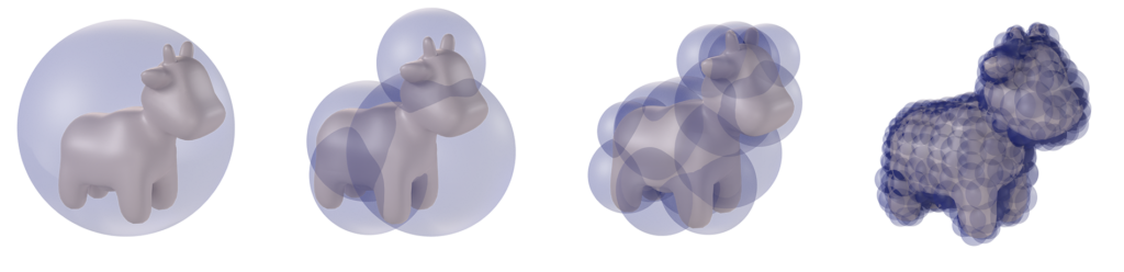
Figure 3: Wrapped BD-Tree for Spot at increasing recursion levels.
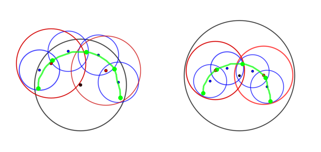
Now that we can compute the minimum bounding spheres for any set of points, we are ready to construct a hierarchical sphere tree on the undeformed model, after which it can be updated following deformation. First we note that the BD-Tree is a wrapped hierarchy, wherein the bounding spheres tightly enclose the underlying geometry but any bounding sphere at one level need not contain its child spheres. This is different from a layered hierarchy in which spheres must enclose their child spheres, but can fit the underlying geometry more loosely (see Figure 4).
Figure 4: An illustration—re-created from [2] of the wrapped hierarchy (left) and layered hierarchy (right). The underlying geometry is shown in green with five vertices and four edges.
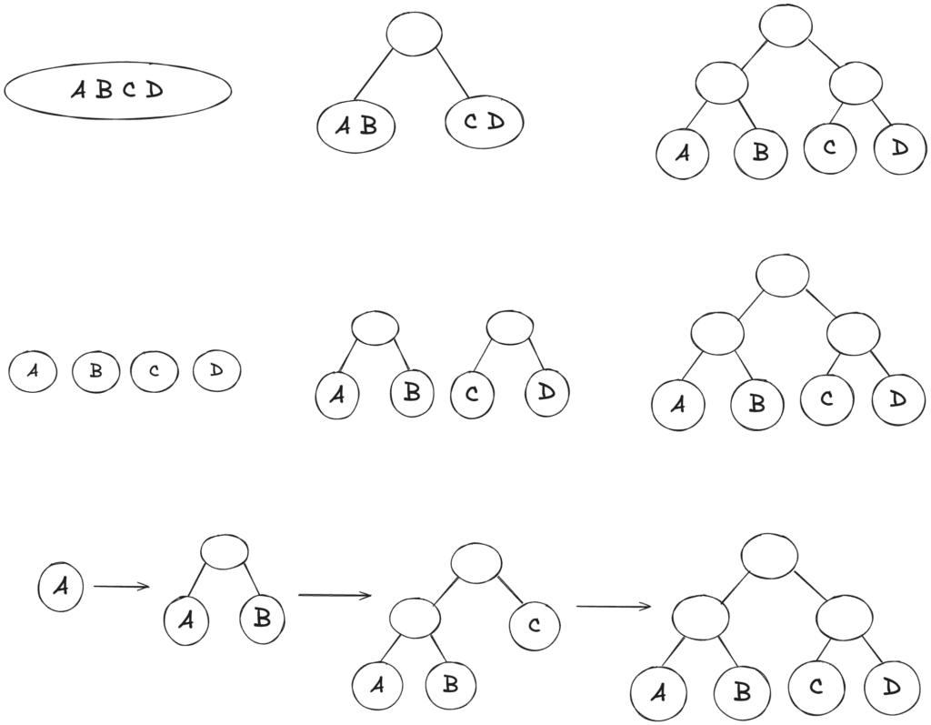
As shown in Figure 5, there are many possible approaches to building a binary tree. In our case, we use a simple top-down approach while partitioning the underlying geometry, i.e. we recursively split Spot at its median into two parts with respect to its local coordination axes, such that a leaf node (the lowest level) contains only one triangle.
Figure 5: Hierarchical binary tree construction with four objects using a top-down (top), bottom-up (middle) and insertion approach (bottom).
As the object deforms, how do we compute the new bounding spheres quickly and efficiently?
Let \(S\) denote a sphere in the hierarchical tree with center \(c\) and radius \(R\) containing the \(k\) points of the geometry \(\{p_{i}\}_{1 \leq i \leq k}\). After the deformation, the center of the sphere \(c\) is displaced by a weighted average of the contained points’ displacements \(u_{i}\) with weights \(\beta_i\) e.g. \(\beta_i := 1/k\) for \(1 \leq i \leq k\). So the new center can be expressed as
\(\displaystyle c’ = c + \sum_{i = 1}^{k} \beta_i u_i.\)
Using the displacement equation above, we can write \(u_i\) as the sum \(\sum_{j = 1}^{r} U_{ij} q_{j}\) and substitute this into the previous equation to obtain:
\(\displaystyle c’ = c + \sum_{j = 1}^{r} \left(\sum_{i = 1}^{k} \beta_i U_{ij}\right) q_j = c + \bar{U} \boldsymbol{q}.\)
To compute the new radius \(R’\), we make use of the triangle inequality
Thus, we have an updated bounding sphere \(S’\) with its center \(c’\) and radius \(R’\) computed as functions of the reduced coordinates \(\boldsymbol{q}\).
Figure 6: Spot colliding with ground plane. The colors of the spheres change based on the ratio of \(R\) in the undeformed state to \(R’\) in the deformed state.
References
[1] Hang Si. TetGen, a Delaunay-based quality tetrahedral mesh generator. ACM Transactions on Mathematical Software, 41(2), 2015.
[2] Doug L. James and Dinesh K. Pai. BD-Tree: Output-Sensitive Collision Detection for Reduced Deformable Models. ACM Transactions on Graphics, 23(3), 2004.
[3] Emo Welzl. Smallest enclosing disks (balls and ellipsoids). New Results and New Trends in Computer Science, 555, 1991.
[4] Christer Ericson. Real-Time Collision Detection. CRC Press, Taylor & Francis Group. Chapter 4, p. 99-100. 2005.
In this three-part series, we rigorously explore the concept of manifolds through the perspectives of both differential geometry and discrete differential geometry. In Part I, we establish the formal definition of a manifold as a special type of topological space and present illustrative examples. In Part II, we introduce the additional structure needed to define differentiable manifolds. Finally, part III presents the discretization of manifolds within the framework of discrete differential geometry, where we approximate smooth manifolds using simplicial complexes or polygonal meshes. Looking at the concept from both perspectives is an opportunity to gain a deeper insight into both types of geometries. The series is nearly self-contained, requiring only a basic understanding of naive set theory and elementary calculus from the reader.
Introduction
A manifold is a special kind of topological space, so special, in fact, that mathematicians have given it its own name. The term “manifold” traces back to the Old English manigfeald and Proto-Germanic maniġfaldaz, meaning “many folds” or “layers.” This etymology descriptively captures the essence of what a manifold represents: a space with many dimensions or complexities, yet with a coherent structure. To define a manifold formally, we first introduce the concept of a general topological space. Only after this, we can talk about the specific properties that a topological space must have to be considered a manifold.
Topological Spaces
Definition. Let \( M \) be a set. Then a choice \( \mathcal{O} \subseteq \mathcal{P}(M) \) is called a topology on \( M \) if:
\( \emptyset \in \mathcal{O} \) and \( M \in \mathcal{O} \);
For any arbitrary collection of sets \( \mathcal{C} \subseteq \mathcal{O}\) \( \Rightarrow \bigcup \mathcal{C} \in \mathcal{O}\)
And the pair \( (M, \mathcal{O}) \) is called a topological space.
Abuse of Notation. In this note, sometimes we abbreviate \(M, \mathcal{O}\) by just \(M\), leaving the topology \( \mathcal{O}\) implicit.
In mathematics, a topology on a set provides the weakest structure needed to define the two very important notions of convergence of sequences to points in a set, and of continuity of maps between two sets. Unless \( |M|=1 \). There are many different topologies one could establish on a set on the same set. Depending on what topology you have on \(M\), the notion of continuity and convergence changes accordingly.
The following table shows us how many different topologies one can establish on a set based on its cardinality.
\( |M| \)
Number of Topologies
1
1
2
4
3
29
4
355
5
6,942
6
209,527
7
9,535,241
Examples of Topologies
Chaotic (trivial) topology: For the set \( M = \{a, b, c\} \), the chaotic topology includes only the entire set and the empty set: \( \mathcal{O} = \{\emptyset, M\} \). This topology is called “chaotic” because it has the least structure, and can be defined on any set.
Discrete Topology: For the set \( M = \{a, b, c\} \), the discrete topology includes every possible subset of \( M \): \( \mathcal{O} = \{\emptyset, \{a\}, \{b\}, \{c\}, \{a, b\}, \{a, c\},\{b, c\}, \{a, b, c\}\}\). This topology provides the most structure, and can be defined on any set.
Standard Topology on \( \mathbb{R} \) (Open Interval Topology): For the set \( M = \mathbb{R} \) (the real numbers), the standard topology is generated by open intervals \( (a, b) \) where \( a, b \in \mathbb{R} \) and \( a < b \): \( \mathcal{O} = \{U \subseteq \mathbb{R} \mid U \text{ is a union of open intervals } (a, b)\}\)
Just as sets are distinguished from each other based on one important property—the cardinality of sets—in set theory, we can define properties that help distinguish one topological space from another. There are many such topological properties for this purpose. We will present those needed to distinguish a topological space that is a manifold from one that is not, namely, the separation, compactness, and paracompactness properties.
Separation, Compactness, and Paracompactness of Topological Spaces
Separation Properties:
Separation properties are used to distinguish points and sets within a topological space, providing a way to understand how “separate” or “distinct” different points or subsets are. To illustrate, consider \(M = \{a, b, c\}\) and the topology \( \mathcal{O} = \{\phi, \{a, b, c\}\}\). This topology is fairly “blind to its element”: it can not tell apart any of the points \(a, b, c\)! But any metric space can tell its points apart (because \(d(x, y) > 0 \) when \( x \neq y\)). While we focus on one specific type of separation property—the \(T_2\) Hausdorff property—there are many other separation properties (many \(Ts\)), some stronger while others are weaker than \(T_2\), that also play important roles in topology.
Definition: A topological space \( (M, \mathcal{O}) \) is called a Hausdorff space (or \(T_2\) space) if for any two distinct points \( p, q \in O \), there exist disjoint open neighborhoods \( U \) and \( V \) such that \( p \in U \) and \( q \in V \). That is, the space satisfies the following condition:
For any \( p, q \in \mathcal{O}\) with \(p \neq q,\) there exist disjoint open sets \(U\) and \(V\) such that \(p \in U\) and \(q \in V. \)
Example: Consider the topological space \( (\mathbb{R}^2, \mathcal{O}) \), where \( \mathcal{O} \) is the standard topology on \( \mathbb{R}^2 \). This space is \(T_2\) Hausdorff. The standard topology \( \mathcal{O} \) on \( \mathbb{R}^2 \) is the collection of all unions of open balls.
An open ball centered at a point \( (x_0, y_0) \) with radius \( r > 0 \) is: \( B((x_0, y_0), r) = \{ (x, y) \in \mathbb{R}^2 \mid \sqrt{(x – x_0)^2 + (y – y_0)^2} < r \} \)
And indeed, \( \mathbb{R}^2 \) has the\(T_2\) (Hausdorff) property since given any two distinct points in \( \mathbb{R}^2 \), you can always find two open balls that do not overlap.
More generally, the topological space \( (\mathbb{R}^d, \mathcal{O} )\) is \(T_2\) Hausdorff where \( \mathcal{O} \) is its standard topology.
Compactness, and Paracompactness:
Definition. Let \( (M, \mathcal{O}) \) be a topological space. An open cover of \( M \) is an arbitrary collection of open sets \( \{ U_{\alpha \in A} \}\) from \( \mathcal{O}\) (possibly infinite or finite) such that: \[ M = \bigcup_{\alpha \in A} U_{\alpha} \]
A subcover is exactly what it sounds like: it takes only some of the \(U_{\alpha \in A}\), while ensuring that \(M\) remains covered.
Definition. A topological space ( \(M, \mathcal{O}\) ) is called compact if every open cover of \( M \) has a finite subcover (i.e. there exists \( F \subset A \) such that: \(M = \bigcup_{\alpha \in F} U_{\alpha}\) where \(F\) is finite).
Compactness is a property that generalizes the notion of closed and bounded sets in Euclidean space. A topological space is compact if every open cover of the space has a finite subcover. This means that, no matter how the space is covered by open sets, it is possible to select a finite number of those sets that still cover the entire space. Compact spaces have several important properties.
In many mathematical contexts, when developing and proving new theorems within the framework of topological spaces, it is common to first address the case where the space is compact. Once the theorem/proof is established for compact spaces, efforts are then made to extend the result to non-compact spaces. Sometimes it is not possible to do the extension. On the other hand, paracompactness is a generalization of compactness (i.e, a much weaker notion) and rarely is it the case to find a topological space that is not paracompact.
Paracompactness:
Definition. A topological space \( (M, \mathcal{O}) \) is called paracompact if every open cover has an open refinement that is locally finite.
Given an open cover \( \{ U_{\alpha \in A} \}\) of \(M\), an open refinement \( { V_{\beta} }_{\beta \in B} \) of this cover is another open cover where every \( V_{\beta} \) is contained in some \( U_{\alpha} \) (i.e. \(\{ V_{\beta} \}_{\beta \in B}\) is a refinement if \( V_{\beta} \subset U_{\alpha} \text{ for some } \alpha \in A.\))
In other words, \( { V_{\beta} }_{\beta \in B} \) is a finer cover than \( \{ U_{\alpha \in A} \}\), meaning that each open set in the refinement is more “localized” or “smaller” in some sense compared to the original cover.
Definition. The refinement is said to be locally finite if every point in \( M \) has a neighborhood that intersects only finitely many of the sets \( V_{\beta} \).
This means that around any given point, only a finite number of the open sets in the cover are “active” or have non-empty intersections with the neighborhood.
In summary: Compactness ensures that any cover can be reduced to a finite cover, while paracompactness ensures that any cover can be refined to a locally finite cover. Compactness deals with the ability to reduce the size of a cover, while paracompactness deals with the ability to organize the cover more effectively without too much local overlap.
Now, we are ready to lay down the formal definition of a manifold!
Manifolds
Definition: A paracompact, Hausdorff topological space ( \(M, \mathcal{O}\) ) is called a (d)-dimensional manifold if for every point \( p \in M \), there exists a neighborhood \( U(p) \) of \( p \) and a homeomorphism \( \varphi: U(p) \to \varphi(U(p) ) \subset \mathbb{R}^d \). In this case, we also write dim \(M\)= \( d \).
What are homeomorphisms? Homeomorphism (Homeos) are structure-preserving maps between topological spaces. Formally, we say that a map \( \varphi: (M, \mathcal{O}_M) \to (N, \mathcal{O}_N) \) is called a homeomorphism if it satisfies the following conditions:
\( \varphi: (M, \mathcal{O}_M) \to (N, \mathcal{O}_N) \) is a bijection
\( \varphi: (M, \mathcal{O}_M) \to (N, \mathcal{O}_N) \) is continuous
The inverse map \( \varphi^{-1}: (N, \mathcal{O}_N) \to (M, \mathcal{O}_M) \) is also continuous.
This definition tells us that a d-manifold is a special type of a topological space where we can distinguish between its subspaces, and it gives us two equivalent ways to think about it:
Locally: for any arbitrary point \(p \in M\), you can always find an open set that contains it and this open set can be mapped by some homeo to a subset of \(\mathbb{R}^d\). For example, to someone standing on the surface of the Earth, the Earth looks much like \(\mathbb{R}^2\).
Globally: there exists an open cover \( \{ U_{\alpha \in A} \}\) (possibly infinite) of \(M\) such that every \(U_{\alpha}\) is mapped by some homeo to a subset of \(\mathbb{R}^d\). For example, from outer space, the Earth can be covered by two hemispherical pancakes.
Examples of Manifolds
The sphere \(S^2\) is a 2-manifold: every point in the sphere has a small open neighborhood that looks like a subset of \(\mathbb{R}^2\). One can cover the Earth with just two hemispheres, and each hemisphere is homeomorphic to a disk in \(\mathbb{R}^2\).
The circle \(S^1\) is a 1-manifold; every point has an open neighborhood that looks like an open interval.
The torus \(T^2\), and Klein bottle are 2-manifold too.
A non-example of a topological space that is not a manifold is the \(n\)-dimensional disk \(D^n\), because it has a boundary; points on the boundary do not have open neighborhoods that can be mapped by some homeo to a subset of \(\mathbb{R}^n\).
Definition. The closed n-dimensional disk, denoted by \( D^n \), is defined as the set of all points \( \mathbf{x} \in \mathbb{R}^n \) such that the Euclidean norm of \( \mathbf{x} \) is less than or equal to 1. Formally, \[ D^n = \{ \mathbf{x} \in \mathbb{R}^n \mid |\mathbf{x}| \leq 1 \} \] where \( |\mathbf{x}| = \sqrt{x_1^2 + x_2^2 + \dots + x_n^2} \) is the Euclidean norm of the vector \( \mathbf{x} = (x_1, x_2, \dots, x_n) \).
Additional terminology: Atlases and Charts
The Terminology of a Chart on a \(d\)–manifold:
Let \(M\) be a \(d\)-manifold then, a chart on \(M\) is a pair \( (U, \varphi) \), where:
\( U \) is an open subset of \( M \).
\( \varphi: U \to \varphi(U) \subset \mathbb{R}^d \) (often called the coordinate map or coordinate chart) is a homeomorphism.
The component functions of \( \varphi: U \to \varphi(U) \subset \mathbb{R}^d \) are the mappings:
\[\varphi^{i}: U \to \mathbb{R}\] \[p \mapsto proj_i(\varphi(p))\]
For \(1 \leq i \leq d\), where \(proj_i(\varphi(p))\) is the \(i\)-th component of \( \varphi (p) \in \mathbb{R}^d\).
This means that the map \( \varphi \) takes every point \(p\) in \( U \) and assigns it coordinates \(proj_i(\varphi(p))\) in \( \mathbb{R}^d = \mathbb{R}\times \mathbb{R} \times \dots \times \mathbb{R}\) ) ( \(d\) times) with respect to the chart \((U, \varphi) \).
Remarks.
Notice that the paragraph above does not introduce any new information beyond what is contained in the definition of a \(d\)-topological manifold. This is why a “chart” is more of a terminology than a definition—though it is a useful one.
We can see by now that there can exist a set \( \mathscr{A}\) of charts for each open set in the open cover \( \{ U_{\alpha \in A} \}\) of \(M\), and there will be many charts that overlap because Different charts may be needed to cover the entire manifold because a single chart might not be able to cover the entire surface of a sphere without singularities or overlaps.
Definition. An atlas of a manifold \( M \) is a collection \( \mathscr{A} := \{(U_\alpha, \varphi_\alpha) \mid \alpha \in A\} \) of charts such that:\[\bigcup_{\alpha \in A} U_\alpha = M.\]
Well, where do you think the words “chart” and “atlas” come from? 🙂
So what happens then if charts overlap? A natural map called the transition map displays itself naturally and is always continuous as a result of the original definition of the topological \(d\)-manifold.
Definition. Two charts \((U_1, \varphi_1)\) and \((U_2, \varphi_2)\) are called \(C^0\)-compatible if either:
By definition, one can go from \(U_1\) into \(\varphi_1 (U_1) \subseteq \mathbb{R}^d\), and similarly one can go from \(U_2\) into \(\varphi_2 (U_2) \subseteq \mathbb{R}^d\). For all the points in the \( U_1 \cap U_2 \), one could use either apply \(\varphi_1\) or \( \varphi_2 \) to land in the subsets \( \varphi_1 (U_1 \cap U_2) \) or \( \varphi_2 (U_1 \cap U_2) \) of \( \mathbb{R}^d \). All of a sudden, we constructed a map that goes from \( \varphi_2 \circ \varphi_1^{-1}: \mathbb{R}^d \to \mathbb{R}^d\) and this map is always continuous
This definition seems redundant and this is true, it applies to every pair of charts. However, it is just a “warm up” since we will later refine this definition and define the differentiability of maps on a manifold in terms of \(C^k\)-compatibility of charts.
Example. Consider a 2-dimensional manifold ( M ), such as the surface of a globe (a sphere). One chart ( (U_1, \varphi_1) ) might cover the Northern Hemisphere, with ( \varphi_1 ) assigning each point in ( U_1 ) latitude and longitude coordinates. Another chart ( (U_2, \varphi_2) ) might cover the Southern Hemisphere. In the overlap ( U_1 \cap U_2 ), the transition map ( \varphi_2 \circ \varphi_1^{-1} ) converts coordinates from the Northern Hemisphere chart to the Southern Hemisphere chart.
Remark. The structure of a topological \(d\)-manifold \(M\) allows us to distinguish subspaces (sub-manifolds) from each other and provides the framework to discuss the continuity of functions defined on \(M\). For example, if you have a curve \( c: \mathbb{R} \to M\) on the manifold, a function \( \mu: \mathbb{R} \to M \) or even a map \(\phi: M \to M\) you can talk about the continuity of \(c\), \(\mu\) and \(\phi\). However, the topological structure alone is not sufficient to discuss their differentiability. To do so, we need to impose an additional structure on \(M\), such as a smooth structure, to define and talk about differentiability.
In part II, we will talk more about Differentiable Manifolds.
Bibliography:
Frederic Schuller (Director). (2015, September 22). Topological manifolds and manifold bundles- Lec 06—Frederic Schuller [Video recording]. https://www.youtube.com/watch?v=uGEV0Wk0eIk
Ananthakrishna, G., Conway, A., Ergen, E., Floris, R., Galvin, D., Hobohm, C., Kirby, R., Kister, J., Kosanović, D., Kremer, C., Lippert, F., Merz, A., Mezher, F., Niu, W., Nonino, I., Powell, M., Ray, A., Ruppik, B. M., & Santoro, D. (n.d.). Topological Manifolds.
Munkres, J. R. (2000). Topology (2nd ed.). Pearson.
Chladni patterns are usually created by putting some light, scattered object like sand onto a metal plate. The metal plate is then made to vibrate, which forms different patterns on the plate depending on the frequency of the wave.
Skrodzki et al. (2016) introduce a method to bring Chladni patterns into the third dimension.
Chladni patterns represent the points along which multiple waves meet to form nodes. These nodes are points along the standing wave formed by the combination of waves where a particle has 0 displacement from its mean.
Depending on the boundary condition, the final solution for the Chladni formulation varies. We can choose between Dirichlet or Neumann conditions.
The above is the solution given a Dirichlet boundary condition. To get the solution with a Nuemann boundary condition, it is the same as the above solution, where all the sin functions are cos instead. More details as to the use of amplitudes and wave number are discussed by Skrodzki et al. (2016).
Using the solution, we can use it as an implicit surface for rendering. This can be done using a standard cube marching algorithm.
Outcome
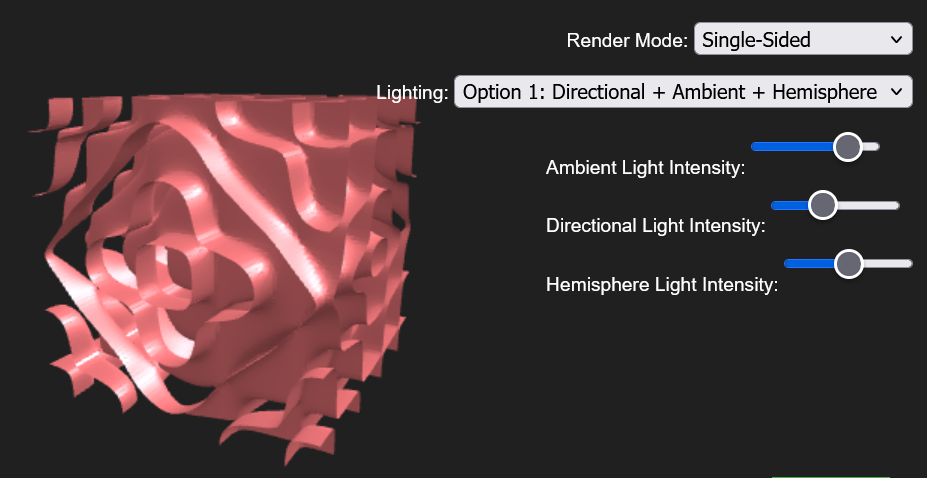
Through the above formulation and cube marching techniques, our group created two open source web versions. A shadertoy implementation as well as a 3js implementation.
Source code and weblinks to both implementations can be seen here.
Image 1: A screenshot of the rendering along with some of the options a user can modify
References
[1] Skrodzki, M., Reitebuch, U., & Polthier, K. (2016). Chladni Figures Revisited: A peek into the third dimension. Proceedings of Bridges 2016: Mathematics, Music, Art, Architecture, Education, Culture, 481–484. http://www.archive.bridgesmathart.org/2016/bridges2016-481.html
This blog was written by Sachin Kishan, Nicolas Pigadas and Bethlehem Tassew during the SGI 2024 Fellowship as one of the outcomes of a one week project under the mentorship of Martin Skrodzki and support of Alberto Tono as teaching assistant.
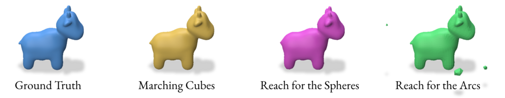
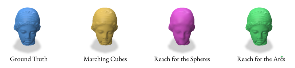
Signed Distance Functions (SDFs) are widely used in computer graphics for rendering and animation. They provide an implicit representation of shapes, which can be converted to explicit representations using methods such as Marching Cubes (MC) and, more recently, Reach for the Spheres (RfS) [Sellan et al. 2023]. However, as we will demonstrate later in this blog post, SDFs have certain limitations in representing various types of surfaces, which can affect the quality of the resulting explicit representations.
Vector Distance Functions (VDFs) [Gomes and Faugeras, 2003] offer a promising alternative, with the potential to overcome some of these limitations. VDFs extend the concept of SDFs by incorporating directional information, allowing for more accurate representation of complex geometries.
This study explores both SDF and VDF-based reconstruction methods, comparing their effectiveness and identifying scenarios where each approach excels. By examining these techniques in detail, we aim to provide insights into their respective strengths and weaknesses, guiding future applications in computer graphics and geometric modeling.
2.0 Reconstruction from SDF
SDFs are one method of representing a surface implicitly. They involve assigning a scalar value to a set of points in a volume. The sign of the SDF value indicates whether the point is inside (-ve) or outside (+ve) the shape, while the magnitude represents the distance to the nearest point on the surface
Mathematically, an SDF \(f(x)\) for a surface \(S\) can be defined as:
$$ f(x) = \begin{cases} -\min_{y \in S} |x – y| & \text{if } x \text{ is inside } S\\ 0 & \text{if } x \text{ is on } S\\ \min_{y \in S} |x – y| & \text{if } x \text{ is outside } S \end{cases} $$
Where, \(|x-y|\) denotes the Euclidean distance between points \(x\) and \(y\).
2.1 Extracting SDF
To reconstruct a surface from an SDF, we first need to obtain SDF values for a set of points in space. There are two main approaches we’ve implemented for sampling these points:
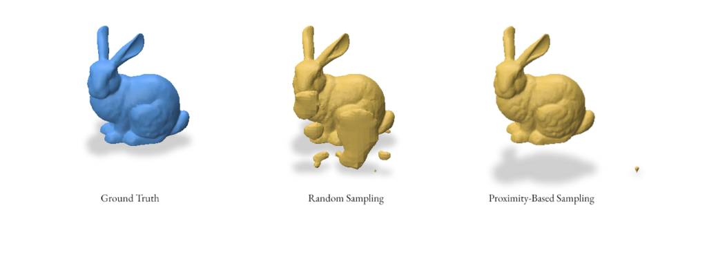
Random Sampling – Generating uniformly distributed random points within a bounding box that encompasses the mesh. This ensures a broad coverage of the space but may miss fine details of the surface.
Proximity-based Sampling – Generating points near the surface of the mesh. This method provides a higher density of samples near the surface, potentially capturing more detail. We implement this by first sampling the points and then adding Gaussian noise to these points.
def extract_sdf(sample_method: SampleMethod, mesh, num_samples=1250000, batch_size=50000, sigma=0.1):
    v, f = gpy.read_mesh(mesh)
    v = gpy.normalize_points(v)

    bbox_min = np.min(v, axis=0)
    bbox_max = np.max(v, axis=0)
    bbox_range = bbox_max - bbox_min
    pad = 0.1 * bbox_range
    q_min = bbox_min - pad
    q_max = bbox_max + pad

    if sample_method == SampleMethod.RANDOM:
        P = np.random.uniform(q_min, q_max, (num_samples, 3))
    elif sample_method == SampleMethod.PROXIMITY:
        P = gpy.random_points_on_mesh(v, f, num_samples)
        noise = np.random.normal(0, sigma * np.mean(bbox_range), P.shape)
        P += noise

    sdf, _, _ = gpy.signed_distance(P, v, f)

    return P, sdf
gpy.random_points_on_mesh() generates points on the mesh surface and gpy.signed_distance() computes the SDF values for the sampled points.
Here’s an example reconstruction using both random and proximity-based sampling for the bunny mesh using the Reach for the Arcs Algorithm:
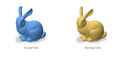
2.2 Reconstruction using Marching Cubes
Marching Cubes is a classic algorithm for extracting a polygonal mesh from an implicit function, such as an SDF. The algorithm works by dividing the space into a regular grid of cubes and then “marching” through these cubes to construct triangles that approximate the surface.
The key steps of the Marching Cubes algorithm are:
Divide the 3D space into a regular grid of cubes.
For each cube:
Evaluate the SDF at each of the 8 vertices.
Determine which edges of the cube intersect the surface (where the SDF changes sign).
Calculate the exact intersection points on the edges using linear interpolation.
Connect these intersection points to form triangles based on a predefined table of cases.
How we implement the marching cubes algorithm in our project:
We first define a bounding box that encompasses all sample points.
We create a regular 3D grid within this bounding box.
We interpolate SDF values onto this regular grid using scipy.interpolate.griddata.
We use the skimage.measure.marching_cubes function to perform the actual Marching Cubes algorithm.
Finally, we scale and translate the resulting vertices back to the original coordinate system.
The Marching Cubes algorithm uses a look-up table to determine how to triangulate each cube based on the sign of the SDF at its vertices. There are 256 possible configurations, which can be reduced to 15 unique cases due to symmetry.
One limitation of the Marching Cubes algorithm is that it can miss thin features or sharp edges due to the fixed grid resolution. Higher resolutions can capture more detail but at the cost of increased computation time and memory usage.
In the next sections, we’ll explore more advanced reconstruction techniques that aim to overcome some of these limitations.
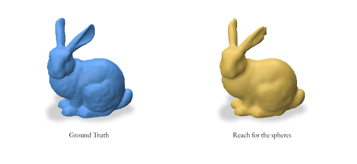
2.3 Reconstruction using Reach for the Spheres
Reach for the Spheres (RFS) is a surface reconstruction method introduced by Sellan et al. in 2023. Unlike Marching Cubes, which operates on a fixed grid, RFS iteratively refines an initial mesh to better approximate the surface represented by the SDF. The key idea behind RFS is to use local sphere approximations to guide the mesh refinement process.
The key steps of the RFS algorithm are:
Start with an initial mesh (typically a low-resolution sphere).
For each vertex in the mesh:
Compute the local reach (maximum sphere radius that doesn’t intersect the surface elsewhere).
Move the vertex to the center of this sphere.
Refine the mesh by splitting long edges and collapsing short ones.
Repeat steps 2-3 for a fixed number of iterations or until convergence.
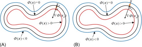
For a vertex \(v\) and its normal \(n\), the local reach \(r\) is computed as:
$$ r = \arg\max_{r > 0} { \forall p \in \mathbb{R}^3 : |p – v| < r \Rightarrow f(p) > -r } $$
Where \(f(p)\) is the SDF value at point \(p\). The new position of the vertex is then:
$$v_{new} = v + r \cdot n$$
How we implement the RFS algorithm in our project:
def reach_for_spheres(self, num_iters=5):
    v_init, f_init = gpy.icosphere(2)
    v_init = gpy.normalize_points(v_init)

    sdf_func = lambda x: griddata(self.pts, self.sdf, x, method='linear', fill_value=np.max(self.sdf))

    for _ in range(num_iters):
        v, f = gpy.reach_for_the_spheres(self.pts, sdf_func, v_init, f_init)
        v_init, f_init = v, f

    return v, f
In this implementation:
We start with an initial icosphere mesh with the subdivision level set to 2 which gives us 162 vertices and 320 faces.
We define an SDF function using interpolation from our sampled points.
We iteratively apply the reach_for_the_spheres function from the gpytoolbox library.
The resulting vertices and faces are used as input for the next iteration.
Based on empirical observations, we’ve found that the best results are achieved when the number of faces and vertices in the initial icosphere is close to, but slightly less than, the expected output mesh complexity. Keeping it greater just simply results in the icosphere as the output.
Subdivision Level (n)
Vertices
Faces
0
12
20
1
42
80
2
162
320
3
642
1280
4
2562
5120
5
10242
20480
6
40962
81920
Subdivision levels of an icosphere and corresponding vertex and face counts generated using the gpy.icosphere function.
Advantages of RFS:
Adaptive resolution: RFS naturally adapts to surface features, using smaller spheres in areas of high curvature and larger spheres in flatter regions.
Feature preservation: The method is better at preserving sharp features compared to Marching Cubes
Topology handling: RFS can handle complex topologies and thin features more effectively than grid-based method.
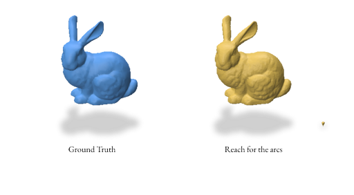
2.4 Reconstruction using Reach for the Arcs
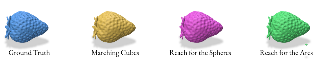
When reconstructing a mesh with Reach for the Arcs (RFA), this algorithm allows us to generate a mesh from a signed distance function. This method is a sort of extension of Reach for the Spheres in the way that it is focused on the curvature of our initial mesh as the focus for the reconstruction. As mentioned in the paper, the run time is slower than reconstructing using Reach for the Sphere but it produces better outputs for closed surfaces with some curvature like spot and strawberry models in Section 2.5.
The key difference between RFA & RFS:
Instead of spheres, we use circular arcs to approximate the local surface.
The algorithm considers the principal curvatures of the surface when determining the arc parameters.
RFA includes additional steps for handling thin features and self-intersections.
For a vertex \(v\) with normal \(n\) and principal curvatures \(\kappa_1\) and \(\kappa_2\), the local arc is defined by:
$$ v(t) = v + r(\cos(t) – 1)n + r\sin(t)d $$
Where \(r = 1/\max(|\kappa_1|, |\kappa_2|)\) is the arc radius, and \(d\) is the direction of maximum curvature.
How we implement the RFA algorithm in our project:
3.0 Reconstruction using VDF (Vector Distance Functions)
Reconstructions using Vector Distance Functions (VDFs) are similar to those using SDFs, except we have added a directional component. After creating a grid of points in a space, we can construct a vector stemming from each point that is both pointing in the direction that minimizes the distance to the mesh, as well as has the magnitude of the SDF at that point. In this way, the tip of each vector will lie on the real surface. From here, we can extract a point cloud of points on the surface and implement a reconstruction method.
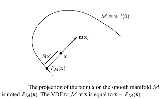
Mathematically, VDF can be used for arbitrary smooth maniform \(M\) with \(k\) dimension.
The following proof is from Gomes and Faugeras’ 2003 paper:
Given a smooth manifold \(M\), which is a subset of \(\mathbb{R}^n\), for every point \(x\), \(\delta(x)\) is that distance of \(\textbf{x}\) to \(M\). Let \(\textbf{u(x)}\) be the vector length of \(\delta(x)\), since \(u(x) = \delta{(x)}D\delta{(x)}\) for \(||D\delta{x}||\)=1. At a point \(\textbf{x}\) where \(\delta \) is differeientable, let \(\textbf{y} = P_{M}(x)\) be an unique projection of \(\textbf{x}\) onto \(M\). This point is such that \(\delta(x) = || x-y||\). Assuming \(M\) is smooth at \(y\), \(\textbf{x-y}\) is normal to \(M\) and parallel to \(D\delta{(x)}\).
Thus:
$$ \textbf{u(x)}= \textbf{x-y}= x-P_{M}(x) $$
Advantages of VDFs:
Due to their directional nature, VDFs have the potential to have more versatility and accuracy compared to SDFs.
There are four main benefits of using VDFs instead of SDFs:
VDFs can be used with shapes with arbitrary codimension.
VDFs perform better mesh reconstruction for closed surfaces.
VDFs can represent open surfaces that SDFs cannot.
VDFs can represent non-manifold surfaces like a Möbius strip.
Disadvantages of VDFs:
Despite these advantages, VDFs do have some drawbacks:
VDFs require more information to be known compared to SDFs
SDFs only need one number (distance) associated with each point in the grid
VDFs, on the other hand, require three numbers (assuming a 3D grid) associated with each point, representing the x, y, and z directions associated with each vector
VDFs can be harder to visualize/debug compared to SDFs
Depending on the method used to obtain them, VDFs can be inaccurate at some grid points
For example, singularities in the gradient can create issues when attempting to use the gradient for a VDF
These inaccurate VDFs can create inaccurate point clouds, which can result in poor reconstructions
Now, we will discuss the methods we used for creating VDFs and using them for reconstructions.
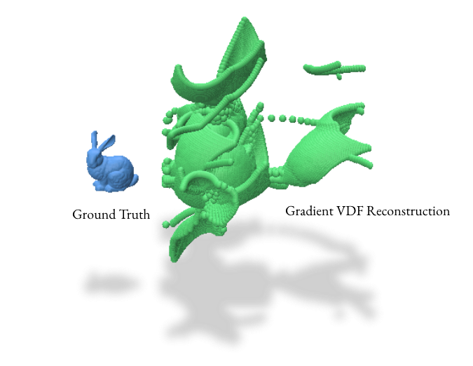
3.1 Reconstruction using Gradient
The gradient-based method leverages the fact that the gradient of a Signed Distance Function (SDF) points in the direction of maximum increase in distance. By reversing this direction and scaling by the SDF value, we obtain vectors pointing towards the surface.
Given an SDF \(\phi(x)\), the VDF \(\mathbf{u}(x)\) is defined as:
This method computes gradients using finite differences, normalizes them, and then scales by the SDF value to obtain the VDF. The surface points are then computed by adding the VDF to the grid vertices.
However, the gradient VDF reconstruction method, while theoretically sound, presented significant practical challenges in our experiments. As evident in the image above, this method produced numerous artifacts and distortions:.These issues likely arise from singularities and numerical instabilities in the gradient field, especially in complex geometries.
Given these results, we opted to focus on the barycentric coordinate method for our VDF reconstructions. This approach proved more robust and reliable, especially for complex 3D models with intricate surface details.
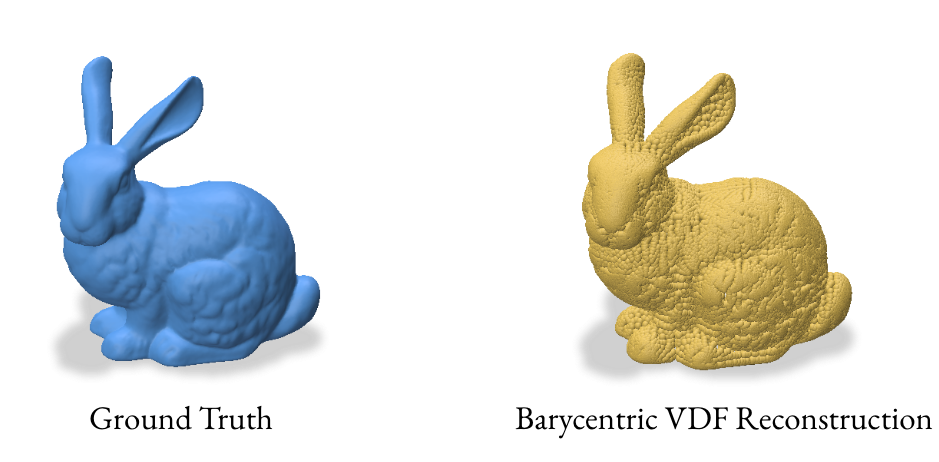
3.2 Reconstruction using Barycentric Coordinates
The barycentric coordinate method utilizes the signed_distance function from gpytoolbox to find the closest points on the mesh for each grid point. These closest points, represented in barycentric coordinates, are then converted to Cartesian coordinates to form a point cloud.
For a point \(p\) with barycentric coordinates \((u, v, w)\) relative to a triangle with vertices \((v_1, v_2, v_3)\), the Cartesian coordinates are:
This method computes the closest points on the mesh for each grid point and converts them to Cartesian coordinates. The VDF is then computed as the normalized vector from the grid point to its closest point on the mesh.
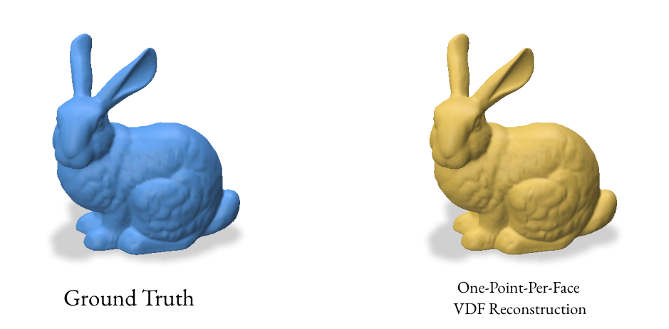
3.3 Reconstruction using one point per face
The one-point-per-face method aims to create a more uniform distribution of points on the surface by using the centroid of each face as a sample point. This approach is particularly effective for meshes with similarly-sized faces.
For a triangle face with vertices \((v_1, v_2, v_3)\), the centroid \(c\) is:
This method computes the centroids and normals for each face of the mesh. It creates a double-sided representation by duplicating the centroids and flipping the normals, which can help in creating a watertight reconstruction.
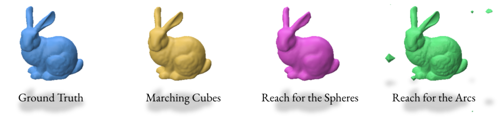
4.0 Analyzing the Results
After performing various reconstruction methods using Signed Distance Functions (SDFs) and Vector Distance Functions (VDFs), it’s crucial to analyze and compare the results. This section covers the visualization, and quantitative evaluation of the reconstructed meshes.
4.1 Visualizing the Results
The project uses the Polyscope library for visualizing the original and reconstructed meshes. The visualize method in all SDFReconstructor, VDFReconstructor and RayReconstructor classes handles the visualization.
This method creates a visual comparison between the original mesh and the reconstructed meshes or point clouds from different methods. The meshes are positioned side by side for easy comparison.
Additionally, the project includes a rendering functionality to export the visualization results as images. This is implemented in the render.py file
4.2 Fitness Score using Chamfer Distance
The project uses the Chamfer distance to compute a fitness score for the reconstructed meshes. The implementation is in the fitness.py file.
The Chamfer distance measures the average nearest-neighbor distance between two point sets. The fitness score is computed as:
This results in a value between 0 and 1, where higher values indicate better reconstruction.
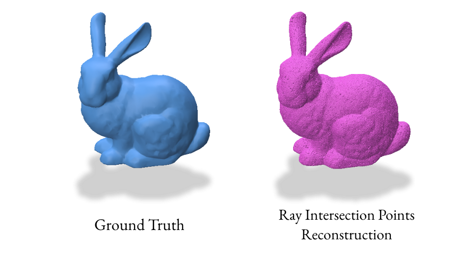
5.0 Some Naive experimentation to get the results
Our initial experiments with the gradient VDF method produced unexpected results due to singularities, leading to inaccurate point clouds. This prompted us to explore alternative VDF methods that directly sample points on the surface, resulting in more reliable reconstructions.
We implemented a ray-based reconstruction technique, the RayReconstructor class, as an additional method. This method generates a point cloud by shooting random rays and finding their intersections with the surface, then uses Poisson Surface Reconstruction to create the final mesh.
6.0 Takeaways & Further Exploration
Overall, VDFs are a promising alternative to SDFs and with the correct reconstruction method, can provide almost identical resultant meshes. They are able to provide more detail at the same resolution when compared to Marching Cubes and Reach for the Spheres. While Reach for the Arcs gives an impressive amount of detail, it often adds too much detail to where it results in details that are not present in the original mesh. VDFs, when constructed/used correctly, do not have this problem. If time permitted, we would have experimented with more non-manifold surfaces and compared the results of SDF and VDF reconstructions of these surfaces. VDFs do not require a clear outside and inside like SDFs do, so we could also explore more such surfaces manifold and non-manifold alike.
Silvia Sellán, Christopher Batty, and Oded Stein. 2023. Reach For the Spheres: Tangency-aware surface reconstruction of SDFs. In SIGGRAPH Asia 2023 Conference Papers (SA ’23). Association for Computing Machinery, New York, NY, USA, Article 73, 1–11. https://doi.org/10.1145/3610548.3618196
Silvia Sellán, Yingying Ren, Christopher Batty, and Oded Stein. 2024. Reach for the Arcs: Reconstructing Surfaces from SDFs via Tangent Points. In ACM SIGGRAPH 2024 Conference Papers (SIGGRAPH ’24). Association for Computing Machinery, New York, NY, USA, Article 23, 1–12. https://doi.org/10.1145/3641519.3657419
José Gomes and Olivier Faugeras. The Vector Distance Functions. International Journal of Computer Vision, vol. 52, no. 2–3, 2003. https://doi.org/10.1023/A:1022956108418
“Since people have tried to prove obvious propositions, they have discovered that many of them are false.” Bertrand Russell
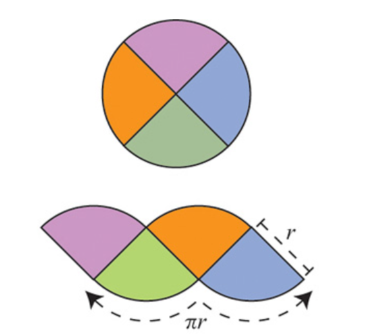
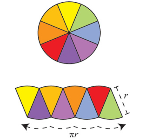
Archimedes proposed an elegant argument indicating that the area of a circle (disk) of radius \(r\) is \( \pi r^2 \). This argument has gained attention recently and is often presented as a “proof” of the formula. But is it truly a proof?
The argument is as follows: Divide the circle into \(2^n\) congruent wedges, and re-arrange them into a strip, for any \( n\) the total sum of the wedges (the area of the strip) is equal to the area of the circle. The top and bottom have arc length \( \pi r \). In the limit the strip becomes a rectangle, meaning as \( n \to \infty \), the wavy strip becomes a rectangle. This rectangle has area \( \pi r^2 \), so the area of the circle is also \( \pi r^2 \).
These images are taken from [1].
To consider this argument a proof, several things need to be shown:
The circle can be evenly divided into such wedges.
The number \( \pi \) is well-defined.
The notion of “area” of this specific subset of \( \mathbb{R}^2 \) -the circle – is well-defined, and it has this “subdivision” property used in the argument. This is not trivial at all; a whole field of mathematics called “Measure Theory” was founded in the early twentieth century to provide a formal framework for defining and understanding the concept of areas/volumes, their conditions for existence, their properties, and their generalizations in abstract spaces.
The limiting operations must be made precise.
The notion of area and arc length is preserved under the limiting operations of 4.
Archimedes’ elegant argument can be rigorised but, it will take some of work and a very long sheet of paper to do so.
Just to provide some insight into the difficulty of making satisfactory precise sense of seemingly obvious and simple-to-grasp geometric notions and intuitive operations which are sometimes taken for granted, let us briefly inspect each element from the above.
Defining \( \pi \):
In school, we were taught that the definition of \( \pi \) is the ratio of the circumference of a circle to its diameter. For this definition to be valid, it must be shown that the ratio is always the same for all circles, which is not immediately obvious; in fact, this does not hold in Non-Euclidean geometry.
A tighter definition goes like this: the number \( \pi \) is the circumference of a circle of diameter 1. Yet, this still leaves some ambiguity because terms like “circumference,” “diameter,” and “circle” need clear definitions, so here is a more precise version: the number \( \pi \) is half the circumference of the circle \( \{ (x,y) | x^2 + y^2 =1 \} \subseteq \mathbb{R}^2 \). This definition is clearer, but it still assumes we understand what “circumference” means.
From calculus, we know that the circumference of a circle can be defined as a special case of arc length. Arc length itself is defined as the supremum of a set of sums, and in nice cases, it can be exactly computed using definite integrals. Despite this, it is not immediately clear that a circle has a finite circumference.
Another limiting ancient argument that is used to estimate and define the circumference of a circle and hence calculating terms of \( \pi \) to some desired accuracy since Archimedes was by using inscribed and circumscribed regular polygons. But still, making a precise sense of the circumference of a circle, and hence the number \( \pi \), is a quite subtle matter.
The Limiting Operation:
In Archimedes’ argument, the limiting operation can be formalized by regarding the bottom of the wavy strip (curve) as the graph of a function \(f_n \), and the limiting curve as the graph of a constant function \(f\). Then \( f_n \to f \) uniformly.
The Notion of Area:
The whole of Euclidean Geometry deals with the notions of “areas” and “volumes” for arbitrary objects in \( \mathbb{R}^2 \) and \( \mathbb{R}^3 \) as if they are inherently defined for such objects and merely need to be calculated. The calculation was done by simply cutting the object into finite simple parts and then rearranging them by performing some rigid motion like rotation or translation and then reassembling those parts to form a simpler body which we already know how to compute. This type of Geometry relies on three hidden assumptions:
Every object has a well-defined area or volume.
The area or volume of the whole is equal to the sum of the areas or volumes of its parts.
The area or volume is preserved under such re-arrangments.
This is not automatically true for arbitrary objects; for example consider the Banach-Tarski Paradox. Therefore, proving the existence of a well-defined notion of area for the specific subset describing the circle, and that it is preserved under the subdivision, rearrangement, and the limiting operation considered, is crucial for validating Archimedes’ argument as a full proof of the area formula. Measure Theory addresses these issues by providing a rigorous framework for defining and understanding areas and volumes. Thus, showing 1,3, 4, and the preservation of the area under the limiting operation requires some effort but is achievable through Measure Theory.
Arc Length under Uniform Limits:
The other part of number 5 is slightly tricky because the arc length is not generally preserved under uniform limits. To illustrate this, consider the staircase curve approximation of the diagonal of a unit square in \( \mathbb{R}^2 \). Even though as the step curves of the staircase get finer and they converge uniformly to the diagonal, their total arc length converges to 2, not to \( \sqrt{2} \). This example demonstrates that arc length, as a function, is not continuous with respect to uniform convergence. However, arc length is preserved under uniform limits if the derivatives of the functions converge uniformly as well. In such cases, uniform convergence of derivatives ensures that the arc length is also preserved in the limit. Is this provable in Archimedes argument? yes with some work.
Moral of the Story:
There is no “obvious” in mathematics. It is important to prove mathematical statements using strict logical arguments from agreed-upon axioms without hidden assumptions, no matter how “intuitively obvious” they seem to us.
“The kind of knowledge which is supported only by observations and is not yet proved must be carefully distinguished from the truth; it is gained by induction, as we usually say. Yet we have seen cases in which mere induction led to error. Therefore, we should take great care not to accept as true such properties of the numbers which we have discovered by observation and which are supported by induction alone. Indeed, we should use such a discovery as an opportunity to investigate more exactly the properties discovered and to prove or disprove them; in both cases we may learn something useful.” –L. Euler
“Being a mathematician means that you don’t take ‘obvious’ things for granted but try to reason. Very often you will be surprised that the most obvious answer is actually wrong.” –Evgeny Evgenievich
Last week, we looked into Voronoi tessellations and their potential for high dimensional sampling and integral approximations.
When we have a very complicated high-dimensional function, it can be very challenging to compute its integral in a given domain. A standard way to approximate it is through Monte Carlo integration
Monte Carlo integration
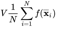
Monte Carlo integration is a technique consisting of querying the integrand function f at Nrandom locations uniformly, taking the average, and then multiplying the region’s volume:
The law of large numbers ensures that, in the limit, this quantity approximates the actual integral better and better.
Okay, but the points are sampled i.i.d. uniformly, which might not be optimal to compute the integral’s value from a very small sample size. Maybe we can find a way to guide the sampling and leverage prior knowledge we might have about the sample space. Okay, and maybe the points are not extracted i.i.d. What if we have no control over the function – maybe it’s some very big machine in a distant factory, or an event occurring once in a decade. If we can’t ensure that the points are i.i.d. we just can’t use Monte Carlo integration.
Therefore, we will investigate whether we can use Voronoi tessellations to overcome this limitation.
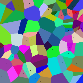
Voronoi Tessellation
A Voronoi tessellation is a partition of the space according to the following rules:
We start with some “pivot” points pi in the space (which could be the points at which we evaluate the integrand function)
Now, we create as many regions as there are initial pivot points defined as follows: a point x in the space belongs to the region of the point pi if the point pi is the closest pivotal point to x :
Voronoi tessellation is essentially one iteration of k-means clustering where the centroids are the pivotal points pi and the data to cluster are all the points x in the domain
Some immediate ideas here:
We can immediately try out “Voronoi integration”, where we multiply the value of the integrand at each starting point f(pi) by the volume of its corresponding region, summing them all up, and see how it behaves compared to Monte Carlo integration (especially in high dimensions)
We can exploit Bayesian optimisation to guide the sampling of the points pi as we don’t require them to be i.i.d. unlike Monte Carlo integration
We can exploit prior knowledge on the integration domain to weight the areas by a measure
In the next blog posts, we will see some of these ideas in action!
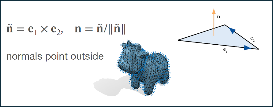
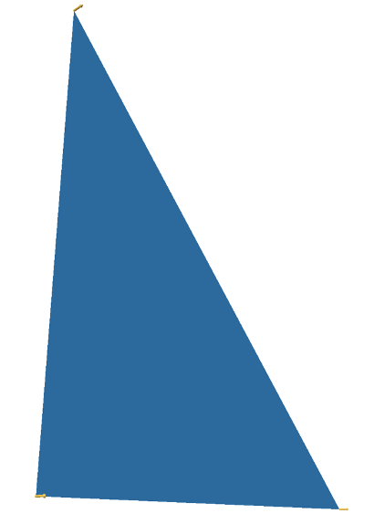
Early in the very first day of SGI, during professor Oded Stein’s great teaching sprint of the SGI introduction in Geometry Processing, we came across normal vectors. As per his slides: “The normal vector is the unit-length perpendicular vector to a triangle and positively oriented”.
Image 1: The formulas and visualisations of normal vectors in professor Oded Stein’s slides.
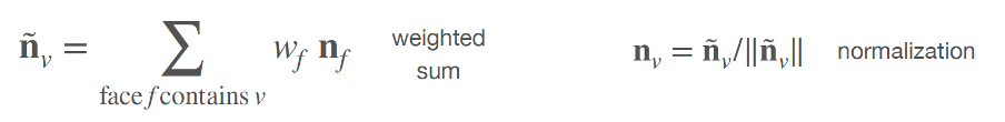
Immediately afterwards, we discussed that smooth surfaces have normals at every point, but as we deal with meshes, it is often useful to define per-vertex normals, apart from the well defined per-face normals. So, to approximate normals at vertices, we can average the per-face normals of the adjacent faces. This is the trivial approach. Then, the question that arises is: Going a step further, what could we do? We can introduce weights:
Image 2: Introducing weights to per-vertex normal vector calculation instead of just averaging the per-face normals. (image credits: professor Oded Stein’s slides)
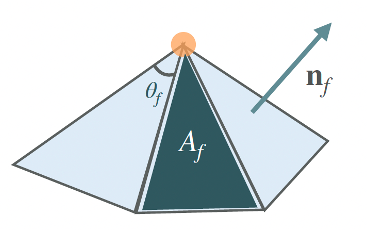
How could we calculate them? The three most common approaches are:
1) The trivial approach: uniform weighting wf = 1 (averaging)
2) area weighting wf = Af
3) angle weighting wf = θf
Image 3: The three most common approaches to calculating weights to perform weighted average of the per-face normals for the calculation of per-vertex normals. (image credits: professor Oded Stein’s slides)
During the talk, we briefly discussed the practical side of choosing among the various types of weights and that area weighting is good enough for most applications and, thus, this is the one implemented in gpytoolbox, a Geometry Processing python package that professor Oded Stein has significantly contributed to its development. Then, he gave us an open challenge: whoever was up for the challenge could implement the angle-weighted per-vertex normal calculation and contribute it to gpytoolbox! I was intrigued and below I give an overview of my implementation of the per_vertex_normals(V, F, weights=’area’, correct_invalid_normals=True) function.
Implementation Overview
First, I implemented an auxiliary function called compute_angles(V,F). This function calculates the angles of each face using the dot product between vectors formed by the vertices of each triangle. The angles are then calculated using the arccosine of the dot product cosine result. The steps are:
For each triangle, the vertices A, B, and C are extracted.
Vectors representing the edges of each triangle are calculated:
AB=B−A
AC=C−A
BC=C−B
CA=A−C
BA=A−B
CB=B−C
The cosine of each angle is computed using the dot product:
cos(α) = (AB AC)/(|AB| |AC|)
cos(β) = (BC BA)/(|BC| |BA|)
cos(γ) = (CA CB)/(|CA| |CB|)
At this point, the numerical issues that can come up in geometry processing applications that we discussed on day 5 with Dr. Nicholas Sharp came to mind. What if the values of arccos(angle) exceed the values 1 or -1? To avoid potential numerical problems I clipped the results to be between -1 and 1:
α=arccos(clip(cos(α),−1,1))
β=arccos(clip(cos(β),−1,1))
γ=arccos(clip(cos(γ),−1,1))
Having compute_angles, now we can explore the per_vertex_normals function. It is modified to get an argument to select weights among the options: “uniform”, “angle”, “area” and applies the selected weight averaging of the per-face normals, to calculate the per-vertex normals:
Make sure that the V and F data structures are of types float64 and int32 respectively, to make our function compatible with any given input
Calculate the per face normals using gpytoolbox
If the selected weight is “area”, then use the already implemented function.
If the selected weight is “angle”:
Compute angles using the compute_angles auxiliary function
Weigh the face normals by the angles at each vertex (weighted normals)
Calculate the norms of the weighted normals
(A small parenthesis: The initial implementation of the function implemented the 2 following steps:
Include another check for potential numerical issues, replacing very small values of norms that may have been rounded to 0, with a very small number, using NumPy (np.finfo(float).eps)
Normalize the vertex normals: N = weighted_normals / norms
Can you guess the problem of this approach?*)
6. Identify indices with problematic norms (NaN, inf, negative, zero)
7. Identify the rest of the indices (of valid norms)
8. Normalize valid normals
9. If correct_invalid_normals == True
Build KDTree using only valid vertices
For every problematic index:
Find the nearest valid normal in the KDTree
Assign the nearest valid normal to the current problematic normal
Else assign a default normal ([1, 0, 0]) (in the extreme case no valid norms are calculated)
Normalise the replaced problematic normals
10. Else ignore the problematic normals and just output the valid normalised weighted normals
*Spoiler alert: The problem of the approach was that -in extreme cases- it can happen that the result of the normalization procedure does not have unit norm. The final steps that follow ensure that the per-vertex normals that this function outputs always have norm 1.
Testing
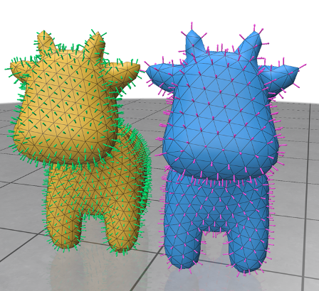
A crucial stage of developing any type of software is testing it. In this section, I provide the visualised results of the angle-weighted per-vertex normal calculations for base and edge cases, as well as everyone’s favourite shape: spot the cow:
Image 4: Let’s start with spot the cow, who we all love. On the left, we have the per-face normals calculated via gpytoolbox and on the right, we have the angle-weighted per-vertex normals, calculated as analysed in the previous section.
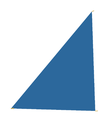
Image 5: The base case of a simple triangle.
Image 6: The base case of an inverted triangle (vertices ordered in a clockwise direction)
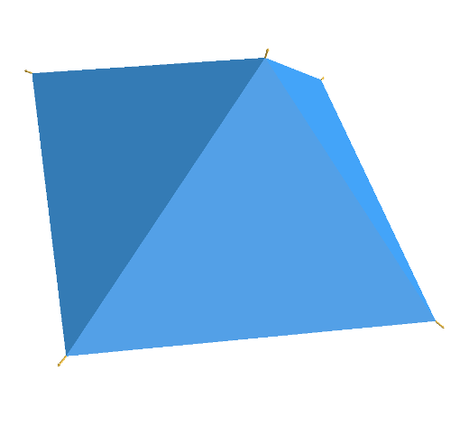
Image 7: The base case of a simple pyramid with a base.
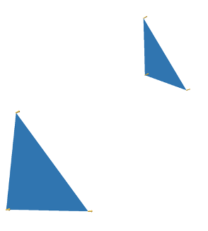
Image 8: The base case of disconnected triangles.
Image 9: The edge case of having a very thin triangle.
Finally, for the cases of a degenerate triangle and repeated vertex coordinates nothing is visualised. The edge cases of having very large or small coordinates have also been tested successfully (coordinates of magnitude 1e8 and 1e-12, respectively).
Having a verified visual inspection is -of course- not enough. The calculations need to be compared to ground truth data in the context of unit tests. To this end, I calculated the ground truth data via the sibling of gpytoolbox: gptoolbox, which is the respective Geometry Processing package but in MATLAB! The shape used to assert the correctness of our per_vertex_normals function, was the famous armadillo. Tests passed for both angle and uniform weights, hurray!
Final Notes
Developing the weighted per-vertex normal function and contributing slightly to such a powerful python library as gpytoolbox, was a cool and humbling experience. Hope the pull request results into a merge! I want to thank professor Oded Stein for the encouragement to take up on the task, as well as reviewing it along with the soon-to-be professor Silvia Sellán!
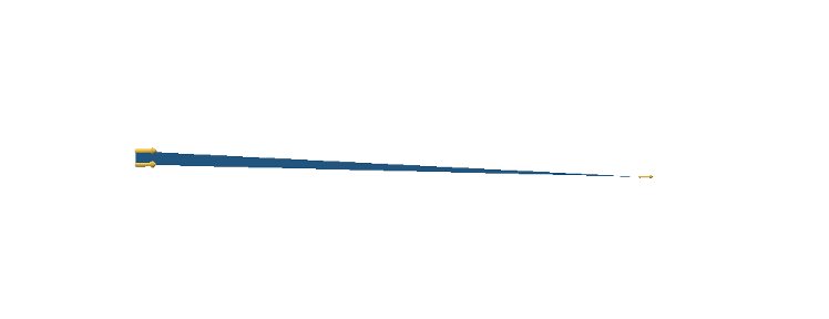
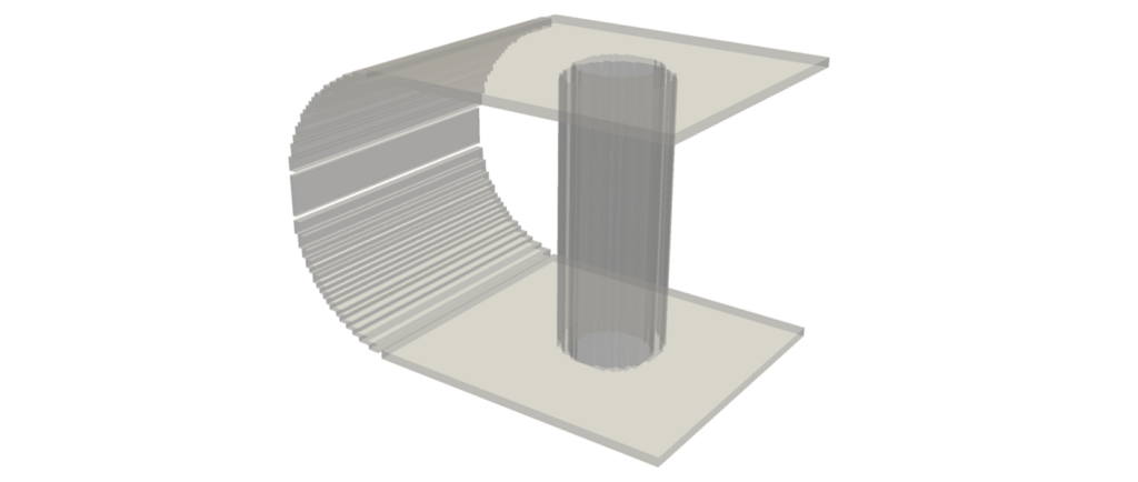
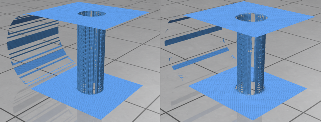
Images: (1) The Wormhole Distance Field (DF) shape. (2) The Wormhole built using DF functions, visualized using a DF/scalar field defined over a discretized space, i.e. a grid. (3) Deploying the marching cubes algorithm (https://dl.acm.org/doi/10.1145/37402.37422) to attempt to reconstruct the surface from the DF shape. (4) Resulting surface using my reconstruction algorithm based on the principles of k-nearest neighbors (kNN), for k=10. (5) Same, but from a different perspective highlighting unreconstructed areas, due to the DF shape having empty areas in the curved plane (see image 2 closely). If those areas didn’t exist in the DF shape, the reconstruction would have likely been exact with smaller k, and thus the representation would have been cleaner and more suitable for ML and GP tasks. (6) The reconstruction for k=5. (7) The reconstruction for k=5, different perspective.
Note: We could use a directional approach to knn for a cleaner reconstructed mesh, leveraging positional information. Alternatively, we could develop a connection correcting algorithm. Irrespectively to if we attempt the aforementioned optimizations or not, we can make the current implementation more optimized, as a lot less distances would need to be calculated after we organize the points of the DF shape based on their positions in the 3D space.
Intro
Well, SGI day 3 came… And it changed everything. In my mind at least. Silvia Sellán and Towaki Takikawa taught us -in the coolest and most intuitive ways- that there is so much more to shape representations. With Silvia, we discussed how one would expect to jump from one representation to another or even try to reconstruct the original shapes from representations that do not explicitely save connectivity information. With Towaki, we discussed Signed Distance Field (SDF) shapes among other stuff (shout out for building a library called haipera, that will definetely be useful to me) and the crazy community building crazy shapes using them. All the newfound knowledge got me thinking. Again.
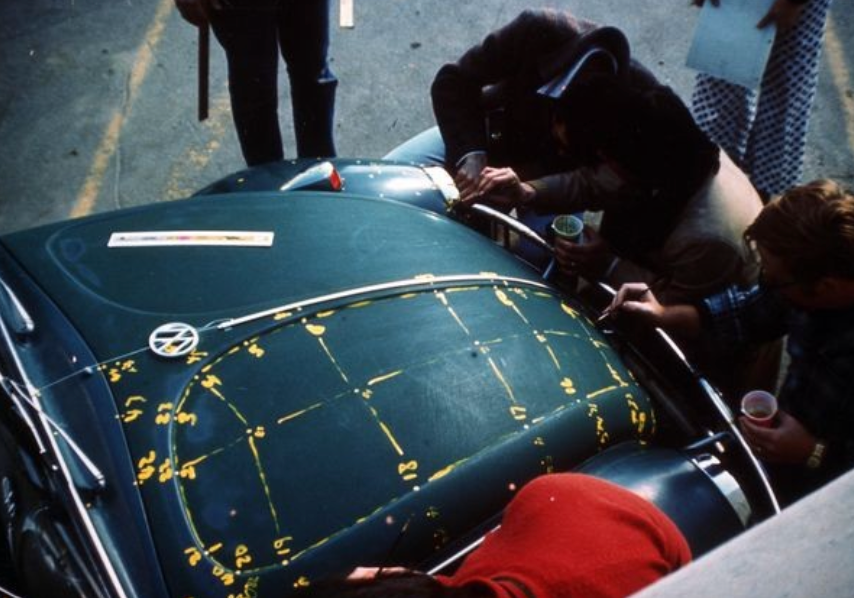
Towaki was asked if there are easier/automated ways to calculate the necessary SDF functions because it would be insane to build -for e.g.- SDF cars by hand. His response? These people are actually insane! And I wanted to get a glimpse of that insanity, to figure out how to build the wormhole using Distance Field (DF) functions. Of course, my target final shape is a lot easier and it turned out that the implementation was far easier than calculating vertices and faces manually (see Wormhole I)! Then, Silvia’s words came to mind: each representation is suitable for different tasks, i.e., a task that is trivial for DF representations might be next to impossible for other representasions. So, creating a DF car is insane, but using functions to calculate the coordinates of a mesh grid car would be even more insane! Fun fact from Silvia’s slides: “The first real object ever 3D scanned and rendered was a WV Beetle by the legendary graphics researcher Ivan Sutherland’s lab (and the car belonged to his wife!)” and it was done manually:
Image (8): Calculating the coordinates of vertices and the faces to design the mesh of a Beetle manually! Geometric Processing gurus’ old school hobbies.
Method
Back to the DF Wormhole. The high-level algorithm for the DF Wormhole is attached below (for the implementation, visit this GitHub repo:
Having my DF Wormhole, the problem of surface reconstruction arose. Thankfully, Silvia had already made sure we got, not only an intuitive understanding of multiple shape representations in 2D and 3D, but also how to jump from one to another and how to reconstruct surfaces from discretized representations. It intrigued me what would happen if I used the marching cubes algorithm on my DF shape. The result was somewhat disappointing (see image 3).
Yet, I couldn’t just let it go. I had to figure out something better. I followed the first idea that came to mind: k-Neirest Neighbors (kNN). My hypothesis was that although the DF shape is in 3D, it doesn’t have any volumetric data. The hypothetical final shape is comprised by surfaces so kNN makes sense; the goal is to find the nearest neighbors and create a mechanism to connect them. It worked (see images 4, 5, 6, 7)! A problem became immediately apparent: the surface was not smooth in certain areas, but rather blocky. Thus, I developed an iterative smoothing mechanism that repositions the nodes based on the average of the coordinates of their neighbors. At 5 iterations the result was satisfying (see image 8). Below I attach the algorithm, (for the implementation, visit this GitHub repo:https://github.com/NIcolasp14/MIT_SGI-Wormhole). Case closed.
Q&A
Q: Why did I call my functions Distance Field functions (DFs) and not Signed Distance Field functions (SDFs)?
A: Because the SDF representation requires some points to have a negative value in relation to a shape’s surface (i.e., we have a negative sign for points inside the shape). In the case of the hollow shapes, such as the hollow cube and cylinder, we replace the negative signs of the inner parts of the outer shapes with positive signs, via the statement max(outer_shape, -inner_shape). Thus, our surfaces/hollow shapes only have 0 values on the surface and positive elsewhere. These type of distance fields are called unsigned (UDFs).
Q: What about the semi-cylinder?
A: The final shape of the semi-cylinder was defined to have negative values inside the radius of the semi-cylinder, 0 on the surface and positive elsewhere. But in order to remove the caps, rather than subtracting an inner cylinder, I gave them a positive value (e.g. infinity). This contradicts the definition of SDFs and UDFs, which measure distance in a continuous way. So, the semi-cylinder would be referred to as a discontinuous distance function (or continuous with specific discontinuities by design).
Future considerations
Using the smoothing mechanism and not using it has a trade off. The smooting mechanism seems to remove more faces -that we do want to have in our mesh-, than if we do not use it (see images 9, 10). The quality of the final surface certaintly depends on the initial DF shape (which indeed had empty spaces, see image 2 closely) and the hyperparameter k of kNN. Someone would need to find the right balance between the aforementioned parameters and the smoothing mechanism or even reconsider how to create the initial Wormhole DF shape or/and how to reposition the vertices, in order to smooth the surfaces more effectively. Finally, all the procedures of the algorithm can be optimized to make the code faster and more efficient. Even the kNN algorithm can be optimized: not every pair must be calculated to compare distances, because we have positional information and thus we can avoid most of the kNN calculations.
Images: (9) Mesh grid using only the mechanism that connects the k-nearest neighbors for k=5, (10) Mesh grid after the additional use of the smoothing mechanism.
Author: Ehsan Shams (Alexandria Univerity, Egypt) Project Mentor: Sofia Di Toro Wyetzner (Stanford University, USA) Volunteer Teaching Assistant: Shanthika Naik (CVIT, IIIT Hyderabad, India)
In my first SGI research week, I went on a fascinating exploratory journey into the world of splines under the guidance of Sofia Wyetzner, and gained an insight into how challenging yet intriguing their construction can be especially under tight constriants such as the requirement for a closed-form expression for their arc-length. This specific construction was the central focus of our inquiry, and the main drive for our exploration.
Splines are important mathematical tools for they are used in various branches of mathematics, including approximation theory, numerical analysis, and statistics, and they find applications in several areas such as Geometry Processing (GP). Loosely speaking, such objects can be understood as mappings that take a set of discrete data points and produce a smooth curve that either interpolates or approximates these points. Thus, it becomes natural immediately to see that they are of great importance in GP since, in the most general sense, GP is a field that is mainly concerned with transforming geometric data1 from one form to another. For example, splines like Bézier and B-spline curves are foundational tools for curve representation in computer graphics and geometric design (Yu, 2024).
Having access to arc lengths for splines in GP is essential for many tasks, including path planning, robot modeling, and animation, where accurate and realistic modeling of curve lengths is critically important. For application-driven purposes, having a closed formula for arc-length computation is highly desirable. However, constructing splines with this arc-length property that can interpolate \( k \) arbitrary data points reasonably well is indeed a challenging task.
Our mentor Sofia, and Shanthika guided us through an exploration of a central question in spline formulation research, as well as several related tangential questions:
Our central question was:
Given \( k \) points, can we construct a spline that interpolates these points and outputs the intermediate arc-lengths of the generated, curve, with some continuity at control points?
And the tangential ones were:
1. Can we achieve \( G^1 \) / \( C^1\) / \( G^2 \) / \(C^2\) continuity at these points with our spline? 2. Given \(k\) points and a total arc-length, can we interpolate these points with the given arc-length in \( \mathbb{R}^2 \)?
In this article, I will share some of the insights I gained from my first week-long research journey, along with potential future directions I would like to pursue.
Understanding Splines and their Arc-length
What are Splines?
A spline is a mapping \( S: [a,b] \subset \mathbb{R} \to \mathbb{R}^n \) defined as:
where \( a = t_0 < t_1 < \cdots < t_n = b \), and \( s_i: [t_i, t_{i+1}] \to \mathbb{R}^n \) are defined such that, \(S(t)\) ensures \( C^k \) continuity at each internal point \( t_j \), meaning:
\( s_{i-1}^{(m)}(t_j) = s_i^{(m)}(t_j) \) for \( m = 0,1 \dots, k \)
where \( s_{i-1}^{(m)} \) and \( s_i^{(m)} \) are the \( m \)-th derivatives of \( s_{i-1}(t) \) and \( s_i(t) \) respectively.
In other words, a spline is a mathematical construct used to create a smooth curve \( S(t) \) by connecting a sequence of simpler piecewise segments \( s_i(t) \) in a continuous manner. These segments \( s_i(t) \) for \( i = 1, 2, \ldots, n \) are defined on subintervals \( [t_i, t_{i+1}] \) of the parameter domain, and are carefully joined end-to-end. The transitions at the junctions \( \{ t_i \}_{i=1}^{n-1} \) (also known as control points) maintain a desired level of smoothness, typically defined by the continuity of derivatives up to order \( k \) on \( \{s_i(t)\}_{i=1}^n \).
One way to categorize splines is based on the types of functions \(s_i\) they incorporate. For instance, some splines utilize polynomial functions such as Bézier splines and B-splines, while others may employ trigonometric functions such as Fourier splines or hyperbolic functions. However, the most commonly used splines in practice are those based on polynomial functions, which define one or more segments. Polynomial splines are particularly valuable in various applications because of their computational simplicity and flexibility in modeling curves.
Arc Length Calculation
Intuitively, the notion of arc-length of a curve2 can be understood as the numerical measurement of the total distance traveled along the curve from one endpoint to another. This concept is fundamental in both calculus and geometry because it provides a way to quantify the length of some curves, which may not be a straight line. To calculate the arc length of smooth curves, we use integral calculus. Specifically, we apply a definite integral formula – (presented in the following theorem) but, let us first define the concept formally.
Definition. Let \( \gamma : [a, b] \to \mathbb{R}^n \) be a parametrized curve, and \( P = \{ a = t_0, t_1, \dots, t_n = b \} \) a partition of \( [a, b] \). The polygonal approximate3 length of \( \gamma \) from \(P\) is given by the sum of the Euclidean distances between the points \( \gamma(t_i)\) for \( i = 0, 1, \dots, n \):
where \( | \cdot | \) denotes the Euclidean norm in \( \mathbb{R}^n \). This polygonal approximation becomes a better estimate of the actual length of the curve as the partition \( P\) becomes finer (i.e., as the maximum distance between successive \( t_i \) tends to zero). The actual length of the curve can be defined as:
\( L(\gamma) = \sup_P L_P(\gamma) \)
If the curve \( \gamma \) is sufficiently smooth, the actual length of the curve can be computed using definite integration as shown in the following theorem.
Arc Length Theorem. Let \( \gamma : [a, b] \to \mathbb{R}^n \) be a \( C^1 \) curve. The arc length \( L(\gamma) \) of \(\gamma\) is given by:
\( L(\gamma) = \int_a^b |\gamma'(t)| \, dt \)
where \(\gamma'(t) \) is the derivative of \(\gamma\) with respect to \(t\).
The challenge
As mentioned earlier, in the context of spline construction for GP tasks, ideally one is interested in constructing splines that have closed-form solutions for their arc length (a formula for computing their arc-length). However, curves with this property for their arc-length are relatively rare because the arc length integral often leads to elliptic integrals4 or other forms that do not have elementary antiderivatives. However, there are some curves for which the arc length can be computed exactly using a closed formula. Here are some examples: Straight lines, circles, and parabolas under certain conditions have closed-form solutions for arc length.
Steps to tackle the central question …
Circular Splines: A Starting Point.
In day one, our mentor Sofia went with us through a paper titled “A Class of \(C^2 \) Interpolating Splines” (Yuksel, 2020). In this work, the author introduces a novel class of non-polynomial parametric splines to interpolate given \( k \) control points. Two components define their class construction: interpolating functions and blending functions (defined later). Each interpolating function \(F_j \in \{F_i \}_{i=1}^n\) defines three consecutive control points, and the blending functions \( \{ B_i \}_{i=1}^m \) combines each two consecutive interpolating functions, forming a smooth curve between two control points. The blending functions are chosen so that \( C^2 \)-continuity everywhere is ensured independent of the choice of the interpolating functions. They use trignometric blending functions.
This type of formulation was constructed to attain some highly desirable properties in the resulting interpolating spline not previously demonstrated by other spline classes, including \( C^2 \) continuity everywhere, local support, and the ability to guarantee self-intersection-free curve segments regardless of the placement of control points and form perfect circular arcs. This paper served as a good starting point in light of the central question under consideration because among the interpolating functions they introduce in their paper are circular curves which have closed formulas for arc-length computation. In addition, it gives insight into the spline formulation practice. However, circular interpolating functions are not without their limitations; their constant curvature makes them difficult to reasonably interpolate arbitrary data, and they look bizarre sometimes.
Interesting note: The earliest documented reference – to the best of my knowledge – discussing the connection of two interpolating curves with a smooth curve dates back to Macqueen’s research in 1936 (MacQueen, 1936) Macqueen’s paper, titled “On the Principal Join of Two Curves on a Surface,” explores the concept of linking two curves on a surface.
Here is a demo constructed by the author to visualize the resulting output spline from their class with different interpolating functions, and below is me playing with the different interpolating functions, and looking at how bizarre the circular interpolating function looks when you throw out data points in an amorphus way.
While playing with the demo, the Gnomus musical track by Modest Mussorgsky was playing in parallel in the back of my mind so I put there for you too. It is a hilarious coincidence that the orchestra goes mad when it is the circular spline’s turn to interpolate the control points, and it does so oddly and bizarrely than the other splines in question. It even goes beyond the boundary of the demo. Did you notice that? 🙂
By the end of the day, I was left with two key inquiries, and a starting point for investigating them:
How do we blend desirable interpolating functions to construct splines with the properties we want? Can we use a combination of circular and elliptical curves to achieve more flexible and accurate interpolation for a wider variety of data points while maintaining a closed form for their arc length? What other combinations could serve us well? I thought to myself: I should re-visit my functional analysis course as a starting point to think about this in a clear way.
From day two to five, we followed a structured yet not restrictive approach, akin to “we are all going to a definite destination but at the same time, everyone could stop by to explore something that captured their attention along the way if they want to and share what intrigued them with others”. This approach was quite effective and engaging:
Implementing a User-Interactive: Our first task was to develop a simple user interface for visualizing existing spline formulations. My SGI project team and friends—Charuka Bandara, Brittney Fahnestock, Sachin Kishan,and I—worked on this in Python (for Catmull-Rom splines) and MATLAB (for Cubic and Quadratic splines). This tool allowed us to visualize how different splines behave and change shape whenever the control points change, also restored my love for coding as I have not coded in a while … you know nothing is more joyful than watching your code executing exactly what you want it to do, right? Below is a UI for visualizing a Cubic Spline. Find the UI for the Quadratic Spline, and the Catmull-Rom here.
Interactive Cubic Spline
Exploring Blending Functions Method: As a natural progression towards our central inquiry, and a complementary task to reading Yuksel’s paper, we eventually found our way to exploring blending functions—a topic I had been eagerly anticipating.
Here, I decided to pause and explore more about the blending function method in spline formulation.
The blending function method, is a method that provides a way to construct a spline \( S(t) \) as a linear combination of a set of control points \( \{p_i(t)\}_{i=1}^n \) and basis functions (blending functions) \( \{B_i(t)\}_{i=1}^n \) in the following manner:
\( S(t) = \sum_{i=1}^n p_i B_i(t)\) (*)
where: \( t \): is the parameter defined over the interval of interest \( [a,b] \)
These blending functions \(B_i(t)\) typically exhibit certain properties that govern, for example, the smoothness, continuity, shape, and preservation of key characteristics that we desire in the resulting interpolating splines. Thus, by carefully selecting and designing those blending functions, it is possible to tailor the behaviour of spline interpolation to meet the specific requirements and achieve desired outcomes.
Below are some of the properties of important blending functions:
Partition of Unity: \( \sum_{i=1}^n B_i(t) =1, \forall t \in [a,b] \), also called coordinate system independent. This property is important because it provides a convex combination of the control points in question, and this is something you need to ensure that the curve does not change if the coordinate changes, one way to visualize this is by imagining that the control points in questions are beads sitting in an amorphous manner on a sheet of paper and the interpolating curve as a thread going through them, and you move the sheet of paper around, what we need is that the thread that goes through these beads does not move around as well, and this is what this property means. Notice that if you pick an arbitrary set of blending functions, this property is not immediately actualized, and the curve would change.
Local Support: Each blending function \( B_i(t) \neq 0 \forall t \in I and i=1,2, … , n \) where \(I \subset [a,b] \) is the interval of interest and vanishes everywhere else on the domain. This property is important because it ensures computational efficiency. With this property actualized in one’s blending functions, one does not have to worry about consequences on their interpolating curve if they are to modify one control point .. for it will only affect a local region in the curve, and not the entire curve.
Non-negativity: Blending functions are often non-negative over the domain of definition \( [a,b] \). This property is called convex hull. It is important for maintaining stability and predictability of the interpolating spline. It prevents the curve from oscillating wildly or provides unfaithful representation of the data point in question.
Smoothness: Blending functions dictate the overall smoothness of the resulting spline since the space of \( C^k (\mathcal{K})\) ( \(k\)-times continously differentiable functions defined on a closed and compact set \(\mathcal{K}\) is a vector space over \(\mathbb{R}\) or \(\mathbb{C}\).
Symmetry: Blending functions that are symmetric about the central control point, do not change if the points are ordered in reverse. In this context, symmetry is assured, if and only if, \( \sum_{i=1}^n B_i(t) p_i = \sum_{i=1}^n B_i ((a+b)-t) p_{n-i} \) this holds if \(B_i(t) = B_{n-i}((a+b)-t) \). For instance, Timmer’s parametric cubic, and Ball’s cubic – (a variant of cubic Bézier) – curve obey this property.
In principle, there can be as many properties imposed on the blending functions depending on the desired aspects one wants in their interpolating spline \( S(t) \).
Remark. The spline formulation (*) describes the weighted sum of the given control points \( \{p_i\}_{i=1}^n\). In other words, each control point is influencing the curve by pulling it in its direction, and the associated blending function is what determines the strength of this influence and pull. Sometimes, one does not need to use blending functions in trivial cases.
Brain-storming for new spline formulation: Finally, we were prepared for our main task. We brainstormed new spline formulations, in doing so, we first looked at different interpolating curves such as catenaries, parabolas, circles for interpolation and arc-length calculation, explored \(C^1\) and \( C^2 \) continuity at control points, did the math on papers, which something I miss nowadays, for the 3-point, and then laid down the foundation for the \(k\)-point interpolation problem. I worked with the parabolas because I love them.
In parallel, I looked a bit into tangential question two … it is an interesting question:
Given \(k\) points and a total arc-length \(L\), can we interpolate these points with the given arc-length in \(\mathbb{R}^2 \)?
From the polynomial interpolation theorem, we know that for any set of \( k \) distinct points \((x_1, y_1), (x_2, y_2), \ldots, (x_k, y_k) \in \mathbb{R}^2 \), there exists a polynomial \( P(x) \) of degree \( k-1 \) such that: \(P(x_i) = y_i \text{ for } i = 1, 2, \ldots, k.\). Such a polynomial is smooth and differentiable (i.e., it is a \( C^\infty \) function) over \( \mathbb{R} \) thus rectifiable so it possesses a well-defined finite arc-length over any closed interval.
Now, let us parameterize the polynomial \( P(x) \) as a parametric curve \( \mathbf{r}(t) = (t, P(t)) \), where \( t \) ranges over some interval \([a, b] \subset \mathbb{R}\).
Now let us compute its arc-length,
The arc-length \( S \) of the curve \( \mathbf{r}(t) = (t, P(t)) \) from \( t = a \) to \( t = b \) is given by:
\( S = \int_a^b \sqrt{1 + \left(\frac{dP(t)}{dt}\right)^2} \, dt. \)
To achieve the desired total arc-length \( L \), we rescale the parameter \( t \). Define a new parameter \( \tau \) as: \( \tau = \alpha t. \)
Now, the new arc-length ( S’ ) in terms of \( \tau \) is:
\(S’ = \frac{S}{\alpha}.\). To ensure \( S’ = L \), choose \( \alpha = \frac{S}{L} \).
Thereby, by appropriately scaling the parameter \( t \), we can adjust the arc-length to match \( L \). Thus, there exists a curve \( C \) that interpolates the \( k \geq 2 \) given points and has the total arc-length \( L \) in \( \mathbb{R}^2 \).
Now, what about implementation? how could we implement an algorithm to execute this task?
It is recommended to visualize your way through an algorithm on a paper first, then formalize to words and symbols, make sure there are no semantic errors in the formalization then code then debug. You know debugging is one of the most intellectually stimulating exercises, and exhausting ones. I am a MATLAB person so here is a MATLAB function you could use to achieve this task ..
function [curveX, curveY] = curveFunction(points, totalArcLength)
    % Input:
    % points - Nx2 matrix where each row is a point [x, y]
    % totalArcLength - desired total arc length of the curve

    % Output:
    % curveX, curveY - vectors of x and y coordinates of the curve

    % Number of points
    n = size(points, 1);

    % Calculate distances between consecutive points
    distances = sqrt(sum(diff(points).^2, 2));

    % Calculate cumulative arc length
    cumulativeArcLength = [0; cumsum(distances)];

    % Normalize cumulative arc length to range from 0 to 1
    normalizedArcLength = cumulativeArcLength / cumulativeArcLength(end);

    % Desired number of points on the curve
    numCurvePoints = 100; % Change as needed

    % Interpolated arc length for the curve
    curveArcLength = linspace(0, 1, numCurvePoints);

    % Interpolated x and y coordinates
    curveX = interp1(normalizedArcLength, points(:, 1), curveArcLength, 'spline');
    curveY = interp1(normalizedArcLength, points(:, 2), curveArcLength, 'spline');

    % Scale the curve to the desired total arc length
    scale = totalArcLength / cumulativeArcLength(end);
    curveX = curveX*scale;
    curveY = curveY*scale;

    %plot(curveX, curveY);

 % Plot the curve
    figure;
    plot(curveX, curveY);
    hold on;
    title('Curve Interpolation using Arc-Length and Points');
    xlabel('X');
    ylabel('Y');
    grid on;
    hold off;
end
Key Takeaways, and Possible Research Directions:
Key Takeaway:
Splines are important!
Constructing them is nontrivial especially under multiple conflicting constraints, as it significantly narrows the feasible search space of potential representative functions.
Progress in abstract mathematics makes the lives of computational engineers and professionals in applied numerical fields easier, as it provides them with greater spaces for creativity and discoveries of new computational tools.
Possible Future Research Directions:
“I will approach this question as one approaches a
hippopotamus: stealthily and from the side.”
– R. Mahony
I borrowed this quote from Prof. Justin Solomon’s Ph.D. thesis. I read parts of it this morning and found that the quote perfectly captures my perspective on tackling the main question of this project. In this context, the “side” approach would involve exploring the question through the lens of functional analysis. 🙂
Acknowledgments. I would like to express my sincere gratitude to our project mentor Sofia Di Toro Wyetzner and Teaching Assistant Shanthika Naik for their continuous support, guidance, and insights to me and my project fellows during this interesting research journey, which prepared me well for my second project on “Differentiable Representations for 2D Curve Networks”. Moreover, I would like to thank my team fellows Charuka Bandara, Brittney Fahnestock, and Sachin Kishan for sharing interesting papers which I am planning to read after SGI!
Silva, L. and Gay Neto, A. (2023). Geometry reconstruction based on arc splines with application to wheel-rail contact simulation. Engineering Computations, 40(7/8), 1889-1920. https://doi.org/10.1108/ec-11-2022-0666
Yuksel, C. (2020). A class of c 2 interpolating splines. ACM Transactions on Graphics, 39(5), 1-14. https://doi.org/10.1145/3400301
Geometric data refers to information that describes the shape, position, and properties of objects in space. It includes the following key components: curves, surfaces, meshes, volumes ..etc ↩︎
In this article, when we say curves, we usually refer to parametric curves. However, parametrized curves are not the same as curves in general ↩︎
The term “polygonal approximation” should not be taken too literally; The term suggests that the Euclidean distance between two points \(p\) and \(q\) should be the “straight-line” distance between them. ↩︎
For the past two weeks, our project team mentored by Dr. Ankita Shukla set out to understand the inner workings of OpenAI’s CLIP model. Specifically, we were interested in gaining a mathematical understanding of feature spaces’ geometric and topological properties.
OpenAI’s CLIP (Contrastive Language-Image Pre-Training) is a versatile and powerful model designed to understand and generate text and images. CLIP is trained to connect text and images by learning from a large dataset of images paired with their corresponding textual descriptions. The model is trained using a contrastive learning approach, where it learns to predict which text snippet is associated with which image from a set of possible pairs. This allows CLIP to understand the relationship between textual and visual information.
Figure 1: OpenAI’s CLIP architecture as it appears in the paper. CLIP pre-trains an image encoder and a text encoder to predict which images were paired with which texts in our dataset. Then OpenAI uses this behavior to turn CLIP into a zero-shot classifier. We convert all of a dataset’s classes into captions such as “a photo of a dog” and predict the class of the caption CLIP estimates best pairs with a given image.
CLIP uses two separate encoders: a text encoder (based on the Transformer architecture) and an image encoder (based on a convolutional neural network or a vision transformer). Both encoders produce embeddings in a shared latent space (also called a feature space). By aligning text and image embeddings in the same space, CLIP can perform tasks that require cross-modal understanding, such as image captioning, image classification with natural language labels, and more.
CLIP is trained on a vast dataset containing 400 million image-text pairs collected online. This extensive training data allows it to generalize across various domains and tasks. One of CLIP’s standout features is its ability to perform zero-shot learning. It can handle new tasks without requiring task-specific training data, simply by understanding the task description in natural language. More information can be found in OpenAI’s paper.
In our attempts to understand the inner workings of the feature spaces, we employed tools from UMAP, persistence homology, subspace angles, cosine similarity matrices, and Wasserstein distances.
Our Study – Methodology and Results
All of our teammates started with datasets that contained image-caption pairs. We classified images into various categories using their captions and embedded them using CLIP. Then we used UMAP or t-SNE plots to visualize their characteristics.
Figure 2: A screenshot of a UMAP of 1000 images from the Flickr 8k dataset from Kaggle divided into five categories (animal, human, sport, nature, and vehicle) is shown. Here we can also observe that the images (colored) are embedded differently than their corresponding captions (gray). Although not shown here, the captions are also clustered around categories.
After this preliminary visualization, we desire to delve deeper. We introduced noise, a Gaussian blur, to our images to test CLIP’s robustness. We added the noise in increments (for example mean = 0, standard deviation = {1,2,3,4,5}) and encoded them as we did the original image-caption pairs. We then made persistence diagrams using ripser. We also followed the same procedure within the various categories to understand how noise impacts not only the overall space but also their respective subspaces. These diagrams for the five categories from the Flickr 8k dataset can be found in this Google Colab notebook.
Figure 3: The same 1000 images from the Flickr 8k dataset with increasing noise are seen above. Visually, no significant difference can be observed. The standard deviation of the Gaussian blur increases from left to right.
Visually, you can observe that there is no significant difference, which attests to CLIP’s robustness. However, visual assurance is not enough. Thus, we used Scipy’sWasserstein’s distance calculation to note how different each persistence diagram is from the other. Continuing the same Flickr 8k dataset, for each category, we obtain the values shown in Figure 4.
Figure 4: Wasserstein distances in each category. You can see the distance between original images with respect to images with Gaussian blur of std. dev = 1 is not high compared to std. dev = 2 or above. This implies that the original set is not as different from the set of images blurred with std. dev. = 1 as compared to std. dev. = 2 which in turn is not as different as the set of blurred images with std. dev. = 3, and so on. This property holds for all five categories.
Another question to understand is how similar are each of the categories to one another. This question can be answered by calculating the subspace angles. After embedding, each category can be seen as occupying a space that can often be far away from another category’s space– we want to quantify how far away, so we use subspace angles. Results for the Flickr 8k dataset example are shown in Figure 5.
Figure 5: Subspace angles of each category pair in the five categories introduced earlier in the post. All values are displayed in degrees. You can observe that the angle between human- and animal-category images is ~0.92° compared to human and nature: ~2.3°; which makes sense as humans and animals are more similar than humans compared to nature. It is worthwhile to note that the five categories are simplifying the dataset too much as they do not capture the nuances of the captions. More categories or descriptions of categories would lead to higher accuracy in the quantity of the subspace angle.
Conclusion
At the start, our team members were novices in the CLIP model, but we concluded as lesser novices. Through the two weeks, Dr. Shukla supported us and enabled us to understand the inner workings of the CLIP model. It is certainly thrilling to observe how AI around us is constantly evolving, but at the heart of it is mathematics governing the change. We are excited to possibly explore further and perform more analyses.