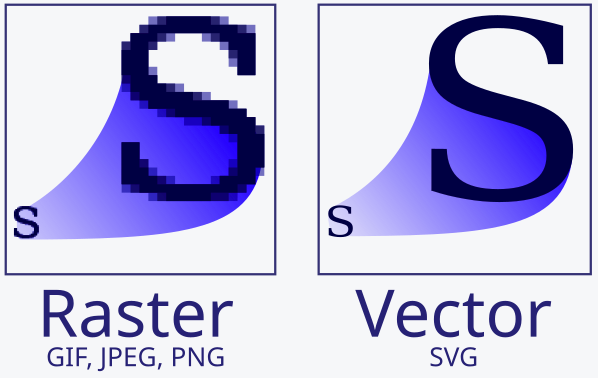
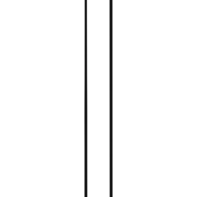
Raster and vector graphics are two fundamental types of image representations used in digital design, each with distinct characteristics and applications. A raster image is a collection of colored pixels in a bitmap, making it well-suited for capturing detailed, complex images like photographs. However, raster graphics provide no additional information about the structure of the object they represent. This limitation can be problematic in scenarios where precision and scalability are essential. For example, representing an artist’s sketch as a raster image may result in jagged curves and the loss of fine details from the original sketch. In such cases, a vector graphics representation is preferred. Unlike raster images, vector graphics use mathematical equations to define shapes, lines, and curves, allowing unlimited scalability without losing quality. This makes vector graphics ideal for logos, illustrations, and other designs where clarity and precision are crucial, regardless of size.
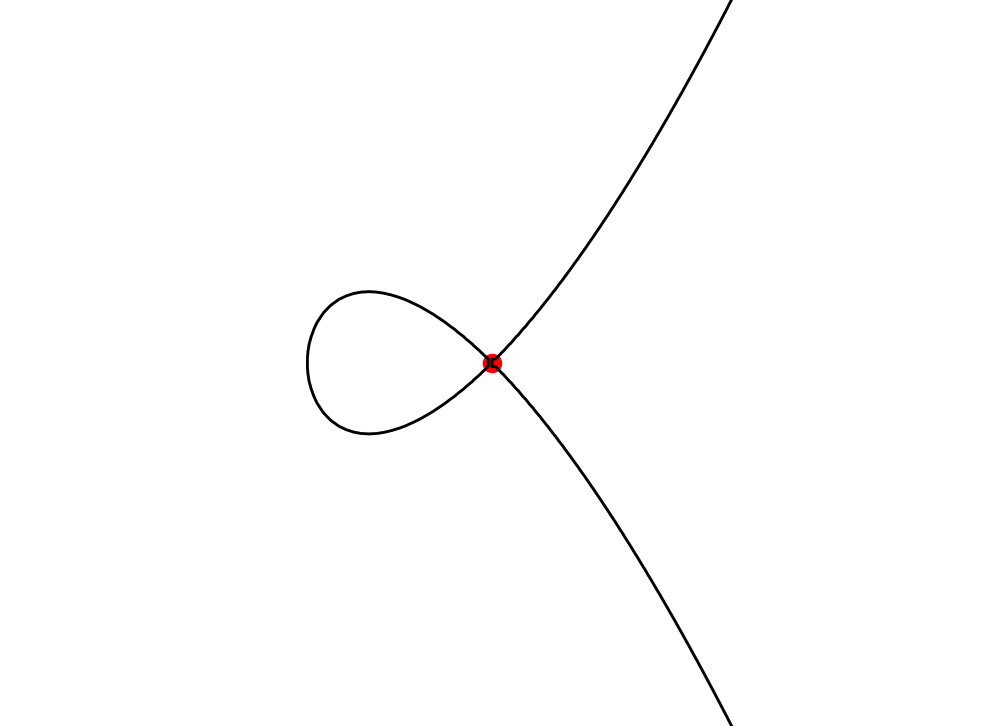
In this project, we aimed to obtain a vector graphics representation of a given sketch in raster form using bicubic curves. A bicubic curve is a polynomial of the form
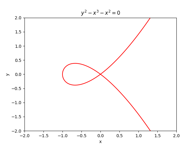
The value a bicubic function takes on a given grid cell is assumed to be uniquely determined by the value the function and its derivatives take at the vertices of the cell. Using bicubic curves allows us to more easily handle self-intersections and closed curves. Additionally, we can create discontinuities at the edges of grid cells by adding some noise to the given bicubic function. This will enable us to vectorize not only smooth but also discontinuous sketches.
A bicubic curve with a self-intersection at (0, 0)
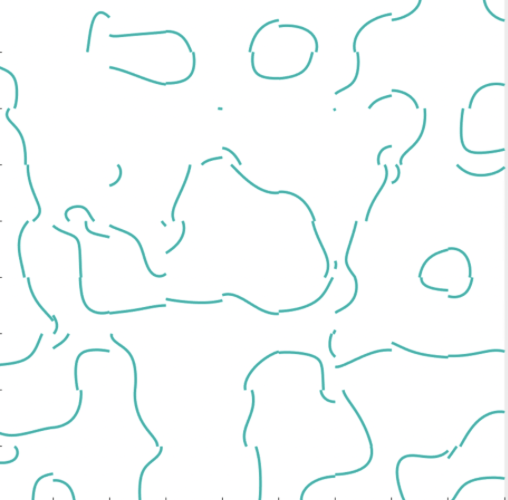
Adding discontinuities at the grid cell edges
Preliminary Work
During the first week of the project, we implemented the following using Python:
For any given grid cell, given its size and the function value p(v) as well as the derivatives px(v), py(v), and pxy(v) at each vertex v, we reconstructed and plotted the unique bicubic function satisfying these values. This reduces to solving a system of sixteen linear equations, following the steps mentioned in the “Bicubic Interpolation” Wikipedia page {4}.
We added noise to the bicubic functions in each cell to create discontinuities. We also found the endpoints of curves in the grid due to the discontinuities formed above.
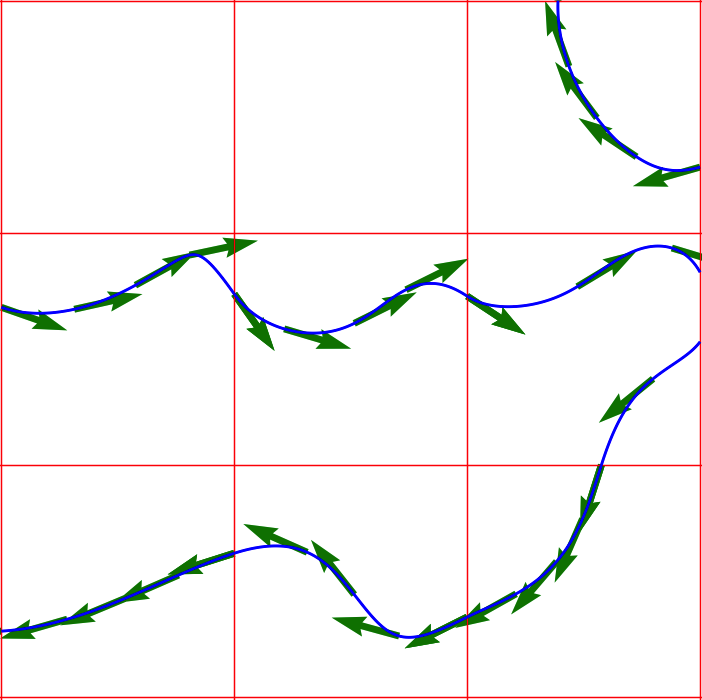
At each point in the grid, we found the gradient of the bicubic functions using fsolve {5} and used them to plot the tangents at some points on the curves.
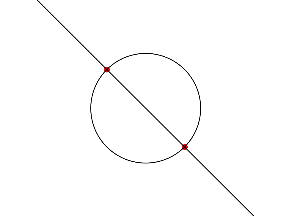
We looked for self-intersections within a grid cell by finding saddle points of the bicubic function (such that the function value is 0 there). If the function is factorizable, it suffices to find the points of intersections between the 0-levels of two or more factors. Here too, we used fsolve.
Bicubic curves with tangents produced by picking four random values between -1 and 1 at each vertex
Bicubic curves with self-intersections marked
Optimization and Rendering
Vectorization
During the second week of the project, I attempted to vectorize the bitmap image by minimizing a function known as the L2 loss.
The L2 loss between the predicted and target bitmap images is computed as the sum of the squared differences for each pixel. To account for this, I gave the bicubic curves some thickness by replacing the curve Z = 0 (here Z = p(x, y) is a bicubic function) in each grid cell with the image of the function e-Z². This allowed me to determine the color at each point in the grid, defining the color of each pixel as the color at its center. Additionally, I calculated the gradient of the color at each point in a grid cell with respect to the coordinates of the corresponding bicubic curve. Using this approach, I defined the L2 loss function and its gradient as follows:
# Defining the loss function
def L2_loss(coeffs, d, width, height, x, y):
    c = np.zeros((height, width))
    for i in range(height):
        for j in range(width):
            c[i, j] = np.exp(-bicubic_function(x[j], y[i], coeffs) ** 2)
    return np.sum((c - d) ** 2)

# Derivative of c(x, y) wrt to the coeff of the x ** m * y ** n term
def colour_gradient(x, y, coeffs, m, n):
    return np.exp(-bicubic_function(x, y, coeffs) ** 2) * (-2 * bicubic_function(x, y, coeffs) * x ** m * y ** n)

# Gradient of the loss function
def gradient(coeffs, d, width, height, x, y):
    grad = np.zeros(16,)
    c = np.zeros((height, width))
    for i in range(height):
        for j in range(width):
            c[i, j] = np.exp(-bicubic_function(x[j], y[i], coeffs) ** 2)
            for n in range(4):
                for m in range(4):
                    k = m + 4 * n
                    grad[k] += 2 * (c[i, j] - d[i, j]) * colour_gradient(x[j], y[i], coeffs, m, n)
    return grad
In this code, d is the normalized numpy array of the target image and x and y are the lists of the x- and y-coordinates of the corresponding pixel centers.
Minimizing this L2 loss in each grid cell gives the vectorization that best approximates the target raster image.
Results
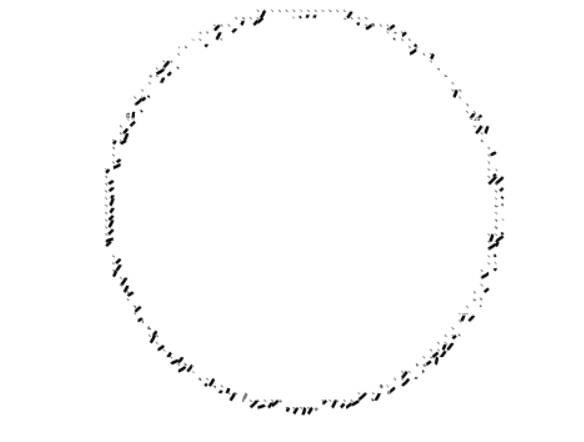
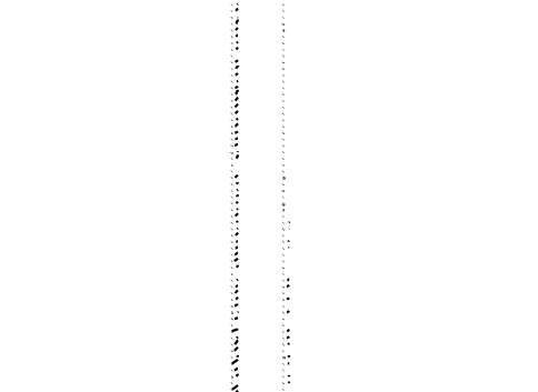
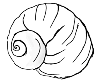
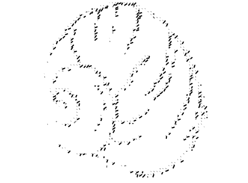
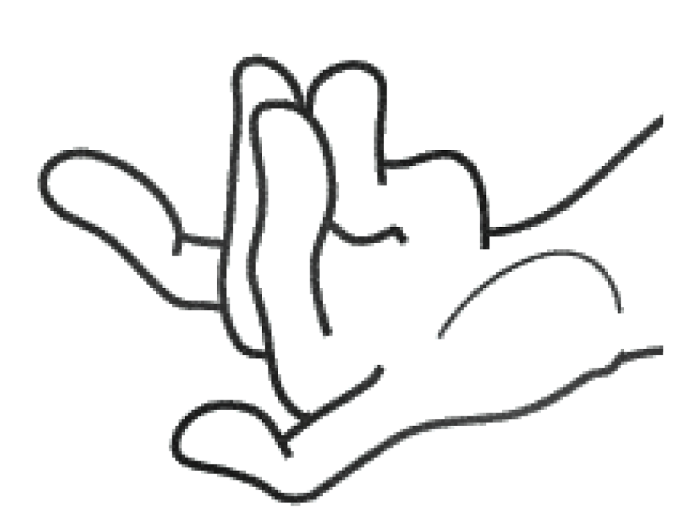
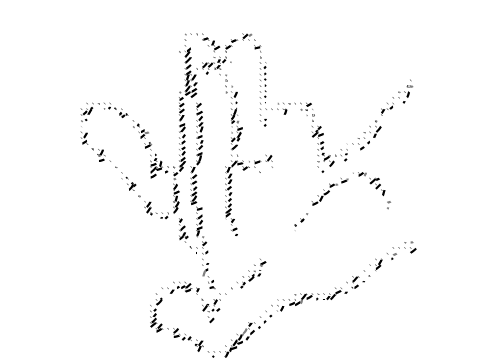
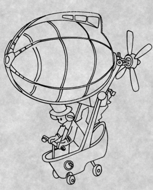
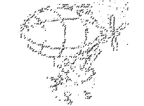
Below are some test bitmap images and their vectorized outputs.
Though the curves mimic the structure of the original sketch, they are not always in the same direction as in the actual sketch. It seems like the curves assume this orientation to depict the thickness of the sketch lines.
Conclusion
Our initial plan was to utilize the code developed in the first week to create a differentiable vectorization. This approach would involve differentiating the functions we wrote to find the endpoints and intersections with respect to the coefficients of the bicubic curve. We would also use the tangents we calculated to determine the curve that best fits the original sketch.
Throughout the project, we worked with bicubic curves to ensure intersections and continuity of isolines between adjacent grid cells. However, we suspect that biquadratic curves might be sufficient for our needs and could significantly improve the implementation’s effectiveness. We are yet to confirm this and also explore whether an even lower degree might be feasible.
This project has opened up exciting avenues for future work and the potential to refine our methods further promises valuable contributions to the field. I am deeply grateful to Mikhail and Daniel for their guidance and support throughout this project.
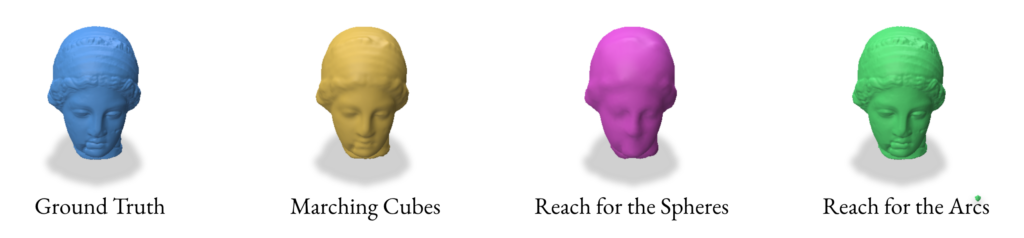
Signed Distance Functions (SDFs) are widely used in computer graphics for rendering and animation. They provide an implicit representation of shapes, which can be converted to explicit representations using methods such as Marching Cubes (MC) and, more recently, Reach for the Spheres (RfS) [Sellan et al. 2023]. However, as we will demonstrate later in this blog post, SDFs have certain limitations in representing various types of surfaces, which can affect the quality of the resulting explicit representations.
Vector Distance Functions (VDFs) [Gomes and Faugeras, 2003] offer a promising alternative, with the potential to overcome some of these limitations. VDFs extend the concept of SDFs by incorporating directional information, allowing for more accurate representation of complex geometries.
This study explores both SDF and VDF-based reconstruction methods, comparing their effectiveness and identifying scenarios where each approach excels. By examining these techniques in detail, we aim to provide insights into their respective strengths and weaknesses, guiding future applications in computer graphics and geometric modeling.
2.0 Reconstruction from SDF
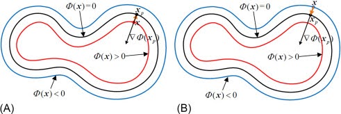
SDFs are one method of representing a surface implicitly. They involve assigning a scalar value to a set of points in a volume. The sign of the SDF value indicates whether the point is inside (-ve) or outside (+ve) the shape, while the magnitude represents the distance to the nearest point on the surface
Mathematically, an SDF \(f(x)\) for a surface \(S\) can be defined as:
$$ f(x) = \begin{cases} -\min_{y \in S} |x – y| & \text{if } x \text{ is inside } S\\ 0 & \text{if } x \text{ is on } S\\ \min_{y \in S} |x – y| & \text{if } x \text{ is outside } S \end{cases} $$
Where, \(|x-y|\) denotes the Euclidean distance between points \(x\) and \(y\).
2.1 Extracting SDF
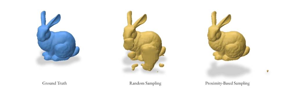
To reconstruct a surface from an SDF, we first need to obtain SDF values for a set of points in space. There are two main approaches we’ve implemented for sampling these points:
Random Sampling – Generating uniformly distributed random points within a bounding box that encompasses the mesh. This ensures a broad coverage of the space but may miss fine details of the surface.
Proximity-based Sampling – Generating points near the surface of the mesh. This method provides a higher density of samples near the surface, potentially capturing more detail. We implement this by first sampling the points and then adding Gaussian noise to these points.
def extract_sdf(sample_method: SampleMethod, mesh, num_samples=1250000, batch_size=50000, sigma=0.1):
    v, f = gpy.read_mesh(mesh)
    v = gpy.normalize_points(v)

    bbox_min = np.min(v, axis=0)
    bbox_max = np.max(v, axis=0)
    bbox_range = bbox_max - bbox_min
    pad = 0.1 * bbox_range
    q_min = bbox_min - pad
    q_max = bbox_max + pad

    if sample_method == SampleMethod.RANDOM:
        P = np.random.uniform(q_min, q_max, (num_samples, 3))
    elif sample_method == SampleMethod.PROXIMITY:
        P = gpy.random_points_on_mesh(v, f, num_samples)
        noise = np.random.normal(0, sigma * np.mean(bbox_range), P.shape)
        P += noise

    sdf, _, _ = gpy.signed_distance(P, v, f)

    return P, sdf
gpy.random_points_on_mesh() generates points on the mesh surface and gpy.signed_distance() computes the SDF values for the sampled points.
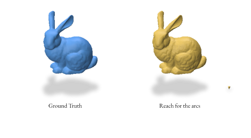
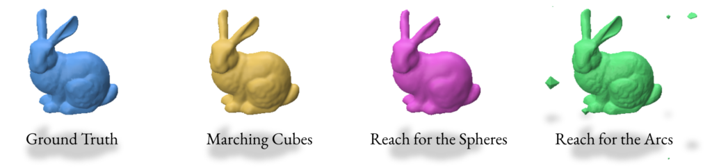
Here’s an example reconstruction using both random and proximity-based sampling for the bunny mesh using the Reach for the Arcs Algorithm:
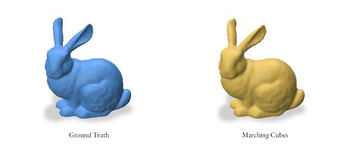
2.2 Reconstruction using Marching Cubes
Marching Cubes is a classic algorithm for extracting a polygonal mesh from an implicit function, such as an SDF. The algorithm works by dividing the space into a regular grid of cubes and then “marching” through these cubes to construct triangles that approximate the surface.
The key steps of the Marching Cubes algorithm are:
Divide the 3D space into a regular grid of cubes.
For each cube:
Evaluate the SDF at each of the 8 vertices.
Determine which edges of the cube intersect the surface (where the SDF changes sign).
Calculate the exact intersection points on the edges using linear interpolation.
Connect these intersection points to form triangles based on a predefined table of cases.
How we implement the marching cubes algorithm in our project:
We first define a bounding box that encompasses all sample points.
We create a regular 3D grid within this bounding box.
We interpolate SDF values onto this regular grid using scipy.interpolate.griddata.
We use the skimage.measure.marching_cubes function to perform the actual Marching Cubes algorithm.
Finally, we scale and translate the resulting vertices back to the original coordinate system.
The Marching Cubes algorithm uses a look-up table to determine how to triangulate each cube based on the sign of the SDF at its vertices. There are 256 possible configurations, which can be reduced to 15 unique cases due to symmetry.
One limitation of the Marching Cubes algorithm is that it can miss thin features or sharp edges due to the fixed grid resolution. Higher resolutions can capture more detail but at the cost of increased computation time and memory usage.
In the next sections, we’ll explore more advanced reconstruction techniques that aim to overcome some of these limitations.
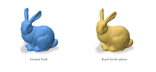
2.3 Reconstruction using Reach for the Spheres
Reach for the Spheres (RFS) is a surface reconstruction method introduced by Sellan et al. in 2023. Unlike Marching Cubes, which operates on a fixed grid, RFS iteratively refines an initial mesh to better approximate the surface represented by the SDF. The key idea behind RFS is to use local sphere approximations to guide the mesh refinement process.
The key steps of the RFS algorithm are:
Start with an initial mesh (typically a low-resolution sphere).
For each vertex in the mesh:
Compute the local reach (maximum sphere radius that doesn’t intersect the surface elsewhere).
Move the vertex to the center of this sphere.
Refine the mesh by splitting long edges and collapsing short ones.
Repeat steps 2-3 for a fixed number of iterations or until convergence.
For a vertex \(v\) and its normal \(n\), the local reach \(r\) is computed as:
$$ r = \arg\max_{r > 0} { \forall p \in \mathbb{R}^3 : |p – v| < r \Rightarrow f(p) > -r } $$
Where \(f(p)\) is the SDF value at point \(p\). The new position of the vertex is then:
$$v_{new} = v + r \cdot n$$
How we implement the RFS algorithm in our project:
def reach_for_spheres(self, num_iters=5):
    v_init, f_init = gpy.icosphere(2)
    v_init = gpy.normalize_points(v_init)

    sdf_func = lambda x: griddata(self.pts, self.sdf, x, method='linear', fill_value=np.max(self.sdf))

    for _ in range(num_iters):
        v, f = gpy.reach_for_the_spheres(self.pts, sdf_func, v_init, f_init)
        v_init, f_init = v, f

    return v, f
In this implementation:
We start with an initial icosphere mesh with the subdivision level set to 2 which gives us 162 vertices and 320 faces.
We define an SDF function using interpolation from our sampled points.
We iteratively apply the reach_for_the_spheres function from the gpytoolbox library.
The resulting vertices and faces are used as input for the next iteration.
Based on empirical observations, we’ve found that the best results are achieved when the number of faces and vertices in the initial icosphere is close to, but slightly less than, the expected output mesh complexity. Keeping it greater just simply results in the icosphere as the output.
Subdivision Level (n)
Vertices
Faces
0
12
20
1
42
80
2
162
320
3
642
1280
4
2562
5120
5
10242
20480
6
40962
81920
Subdivision levels of an icosphere and corresponding vertex and face counts generated using the gpy.icosphere function.
Advantages of RFS:
Adaptive resolution: RFS naturally adapts to surface features, using smaller spheres in areas of high curvature and larger spheres in flatter regions.
Feature preservation: The method is better at preserving sharp features compared to Marching Cubes
Topology handling: RFS can handle complex topologies and thin features more effectively than grid-based method.
2.4 Reconstruction using Reach for the Arcs
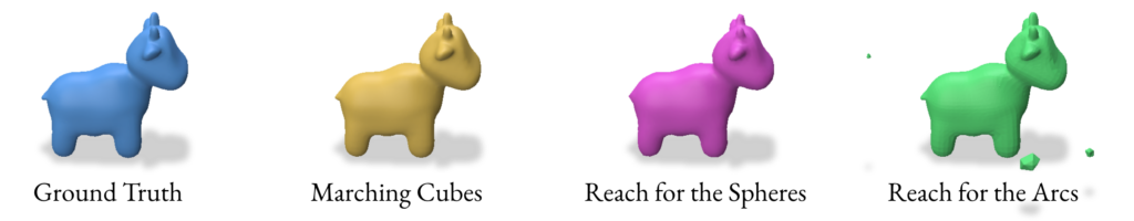
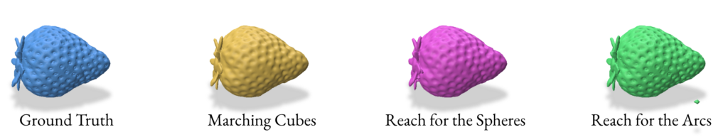
When reconstructing a mesh with Reach for the Arcs (RFA), this algorithm allows us to generate a mesh from a signed distance function. This method is a sort of extension of Reach for the Spheres in the way that it is focused on the curvature of our initial mesh as the focus for the reconstruction. As mentioned in the paper, the run time is slower than reconstructing using Reach for the Sphere but it produces better outputs for closed surfaces with some curvature like spot and strawberry models in Section 2.5.
The key difference between RFA & RFS:
Instead of spheres, we use circular arcs to approximate the local surface.
The algorithm considers the principal curvatures of the surface when determining the arc parameters.
RFA includes additional steps for handling thin features and self-intersections.
For a vertex \(v\) with normal \(n\) and principal curvatures \(\kappa_1\) and \(\kappa_2\), the local arc is defined by:
$$ v(t) = v + r(\cos(t) – 1)n + r\sin(t)d $$
Where \(r = 1/\max(|\kappa_1|, |\kappa_2|)\) is the arc radius, and \(d\) is the direction of maximum curvature.
How we implement the RFA algorithm in our project:
3.0 Reconstruction using VDF (Vector Distance Functions)
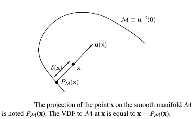
Reconstructions using Vector Distance Functions (VDFs) are similar to those using SDFs, except we have added a directional component. After creating a grid of points in a space, we can construct a vector stemming from each point that is both pointing in the direction that minimizes the distance to the mesh, as well as has the magnitude of the SDF at that point. In this way, the tip of each vector will lie on the real surface. From here, we can extract a point cloud of points on the surface and implement a reconstruction method.
Mathematically, VDF can be used for arbitrary smooth maniform \(M\) with \(k\) dimension.
The following proof is from Gomes and Faugeras’ 2003 paper:
Given a smooth manifold \(M\), which is a subset of \(\mathbb{R}^n\), for every point \(x\), \(\delta(x)\) is that distance of \(\textbf{x}\) to \(M\). Let \(\textbf{u(x)}\) be the vector length of \(\delta(x)\), since \(u(x) = \delta{(x)}D\delta{(x)}\) for \(||D\delta{x}||\)=1. At a point \(\textbf{x}\) where \(\delta \) is differeientable, let \(\textbf{y} = P_{M}(x)\) be an unique projection of \(\textbf{x}\) onto \(M\). This point is such that \(\delta(x) = || x-y||\). Assuming \(M\) is smooth at \(y\), \(\textbf{x-y}\) is normal to \(M\) and parallel to \(D\delta{(x)}\).
Thus:
$$ \textbf{u(x)}= \textbf{x-y}= x-P_{M}(x) $$
Advantages of VDFs:
Due to their directional nature, VDFs have the potential to have more versatility and accuracy compared to SDFs.
There are four main benefits of using VDFs instead of SDFs:
VDFs can be used with shapes with arbitrary codimension.
VDFs perform better mesh reconstruction for closed surfaces.
VDFs can represent open surfaces that SDFs cannot.
VDFs can represent non-manifold surfaces like a Möbius strip.
Disadvantages of VDFs:
Despite these advantages, VDFs do have some drawbacks:
VDFs require more information to be known compared to SDFs
SDFs only need one number (distance) associated with each point in the grid
VDFs, on the other hand, require three numbers (assuming a 3D grid) associated with each point, representing the x, y, and z directions associated with each vector
VDFs can be harder to visualize/debug compared to SDFs
Depending on the method used to obtain them, VDFs can be inaccurate at some grid points
For example, singularities in the gradient can create issues when attempting to use the gradient for a VDF
These inaccurate VDFs can create inaccurate point clouds, which can result in poor reconstructions
Now, we will discuss the methods we used for creating VDFs and using them for reconstructions.
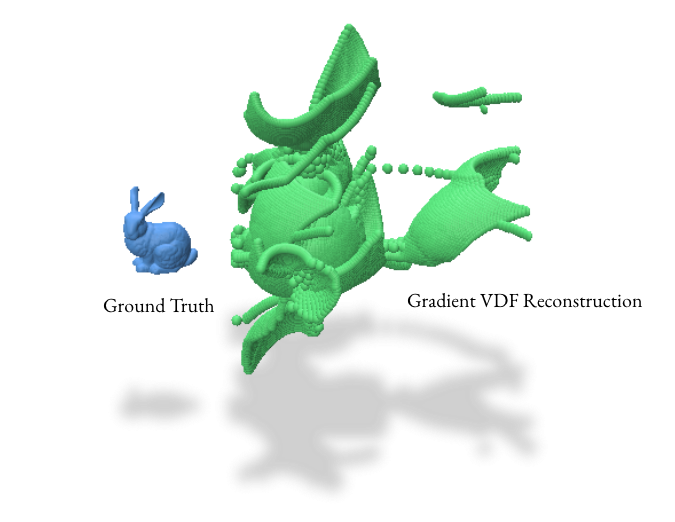
3.1 Reconstruction using Gradient
The gradient-based method leverages the fact that the gradient of a Signed Distance Function (SDF) points in the direction of maximum increase in distance. By reversing this direction and scaling by the SDF value, we obtain vectors pointing towards the surface.
Given an SDF \(\phi(x)\), the VDF \(\mathbf{u}(x)\) is defined as:
This method computes gradients using finite differences, normalizes them, and then scales by the SDF value to obtain the VDF. The surface points are then computed by adding the VDF to the grid vertices.
However, the gradient VDF reconstruction method, while theoretically sound, presented significant practical challenges in our experiments. As evident in the image above, this method produced numerous artifacts and distortions:.These issues likely arise from singularities and numerical instabilities in the gradient field, especially in complex geometries.
Given these results, we opted to focus on the barycentric coordinate method for our VDF reconstructions. This approach proved more robust and reliable, especially for complex 3D models with intricate surface details.
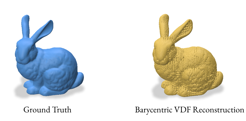
3.2 Reconstruction using Barycentric Coordinates
The barycentric coordinate method utilizes the signed_distance function from gpytoolbox to find the closest points on the mesh for each grid point. These closest points, represented in barycentric coordinates, are then converted to Cartesian coordinates to form a point cloud.
For a point \(p\) with barycentric coordinates \((u, v, w)\) relative to a triangle with vertices \((v_1, v_2, v_3)\), the Cartesian coordinates are:
This method computes the closest points on the mesh for each grid point and converts them to Cartesian coordinates. The VDF is then computed as the normalized vector from the grid point to its closest point on the mesh.
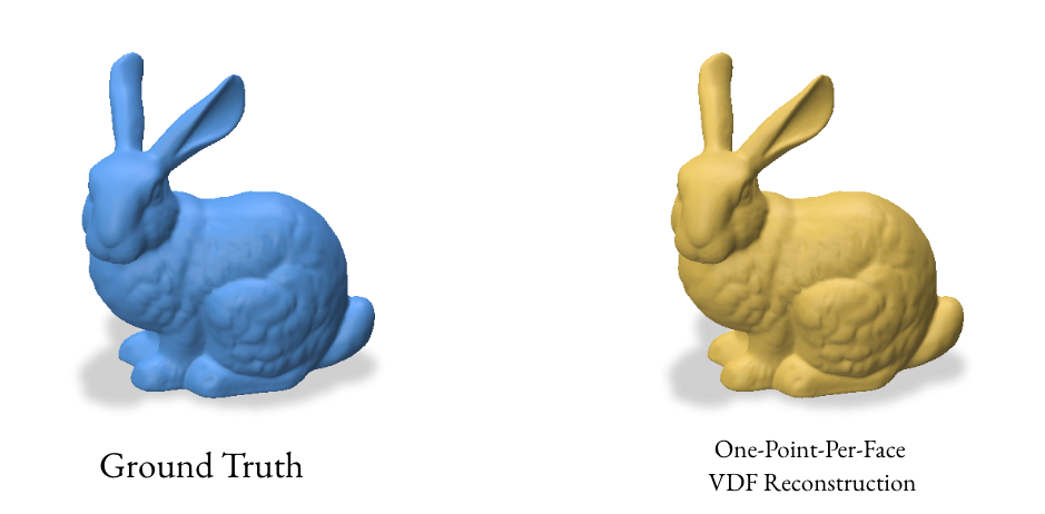
3.3 Reconstruction using one point per face
The one-point-per-face method aims to create a more uniform distribution of points on the surface by using the centroid of each face as a sample point. This approach is particularly effective for meshes with similarly-sized faces.
For a triangle face with vertices \((v_1, v_2, v_3)\), the centroid \(c\) is:
This method computes the centroids and normals for each face of the mesh. It creates a double-sided representation by duplicating the centroids and flipping the normals, which can help in creating a watertight reconstruction.
4.0 Analyzing the Results
After performing various reconstruction methods using Signed Distance Functions (SDFs) and Vector Distance Functions (VDFs), it’s crucial to analyze and compare the results. This section covers the visualization, and quantitative evaluation of the reconstructed meshes.
4.1 Visualizing the Results
The project uses the Polyscope library for visualizing the original and reconstructed meshes. The visualize method in all SDFReconstructor, VDFReconstructor and RayReconstructor classes handles the visualization.
This method creates a visual comparison between the original mesh and the reconstructed meshes or point clouds from different methods. The meshes are positioned side by side for easy comparison.
Additionally, the project includes a rendering functionality to export the visualization results as images. This is implemented in the render.py file
4.2 Fitness Score using Chamfer Distance
The project uses the Chamfer distance to compute a fitness score for the reconstructed meshes. The implementation is in the fitness.py file.
The Chamfer distance measures the average nearest-neighbor distance between two point sets. The fitness score is computed as:
This results in a value between 0 and 1, where higher values indicate better reconstruction.
5.0 Some Naive experimentation to get the results
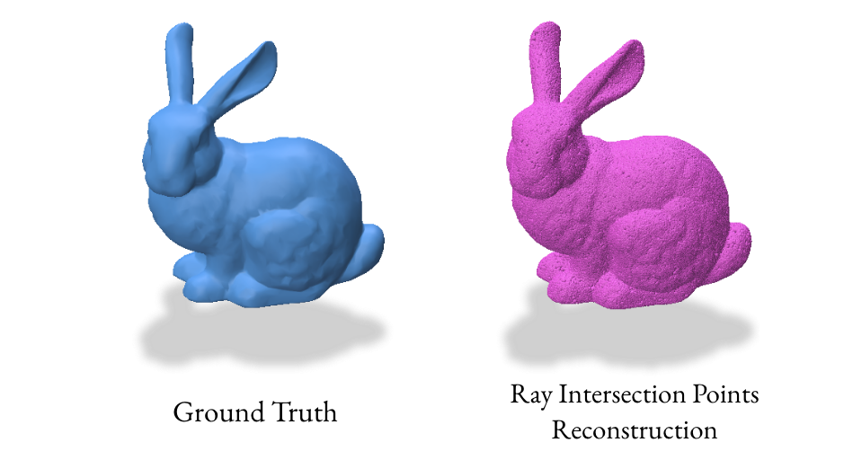
Our initial experiments with the gradient VDF method produced unexpected results due to singularities, leading to inaccurate point clouds. This prompted us to explore alternative VDF methods that directly sample points on the surface, resulting in more reliable reconstructions.
We implemented a ray-based reconstruction technique, the RayReconstructor class, as an additional method. This method generates a point cloud by shooting random rays and finding their intersections with the surface, then uses Poisson Surface Reconstruction to create the final mesh.
6.0 Takeaways & Further Exploration
Overall, VDFs are a promising alternative to SDFs and with the correct reconstruction method, can provide almost identical resultant meshes. They are able to provide more detail at the same resolution when compared to Marching Cubes and Reach for the Spheres. While Reach for the Arcs gives an impressive amount of detail, it often adds too much detail to where it results in details that are not present in the original mesh. VDFs, when constructed/used correctly, do not have this problem. If time permitted, we would have experimented with more non-manifold surfaces and compared the results of SDF and VDF reconstructions of these surfaces. VDFs do not require a clear outside and inside like SDFs do, so we could also explore more such surfaces manifold and non-manifold alike.
Silvia Sellán, Christopher Batty, and Oded Stein. 2023. Reach For the Spheres: Tangency-aware surface reconstruction of SDFs. In SIGGRAPH Asia 2023 Conference Papers (SA ’23). Association for Computing Machinery, New York, NY, USA, Article 73, 1–11. https://doi.org/10.1145/3610548.3618196
Silvia Sellán, Yingying Ren, Christopher Batty, and Oded Stein. 2024. Reach for the Arcs: Reconstructing Surfaces from SDFs via Tangent Points. In ACM SIGGRAPH 2024 Conference Papers (SIGGRAPH ’24). Association for Computing Machinery, New York, NY, USA, Article 23, 1–12. https://doi.org/10.1145/3641519.3657419
José Gomes and Olivier Faugeras. The Vector Distance Functions. International Journal of Computer Vision, vol. 52, no. 2–3, 2003. https://doi.org/10.1023/A:1022956108418
A cool aspect of the SGI is the opportunity to engage with distinguished guest speakers ranging from both industry and academia who deliver captivating talks on topics centered around Geometry Processing. On August 8th, we had the pleasure of hearing from Professor Lining Yao, the director of the Morphing Matter Lab at the University of California Berkeley. Her talk was a captivating journey into the world of morphing materials and their potential impact on sustainable design.
The Intersection of Design and Sustainability
Professor Yao kicked off her talk by discussing her research focus on “morphing materials” — materials that can change properties and shapes in response to environmental stimuli. She emphasized the importance of combining human-centered design with nature-centered principles, a dual approach which aims to create products that not only benefit people but also minimize harm to the environment.
Real-World Applications of Morphing Materials
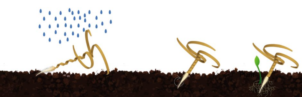
One of the examples Prof. Yao shared was a biodegradable material inspired by the seed of Erodium. This innovative design allows the seed to bury itself into the ground after rain, which enhances its germination rate. This, probably, is a fantastic example of how nature can inspire sustainable technology. She further explained that such self-burying seeds could be used for ecological restoration, which makes them a powerful tool for environmental conservation.
Figure 1: A photo of a seed of Erodium, a genus of plants with seeds that unwind coiled tails to act as a drill to plant into the ground.
Another fascinating application of Morphing Materials is in the realm of 4D printing (an advanced form of 3D printing that incorporates the dimension of time into the manufacturing process, enabling printed objects to change shape or function over time in response to environmental stimuli such as heat, moisture, light, or other factors). Prof. Lining described how self-folding structures could revolutionize manufacturing by reducing material waste and production time. For instance, a flat sheet could be printed and then transformed into a chair, saving both resources and energy.
This short video shows a demonstration 4D printing of Self-folding materials and interfaces.
Professor Lining didn’t stop at serious applications; she also introduced us to the fun and playful side of her research work. Imagine Italian pasta that can morph from a flat shape into various delicious forms when cooked! This innovative approach not only saves packaging space during transportation and storage, but also contributes to reducing plastic waste. This tells us that sustainability can be both functional and fun.
The Video below demonstrates a Flatpack of morphing pasta for sustainable food packaging and greener cooking.
Listening to Professor Yao was indeed exhilarating. Her insights made it clear that the concepts of morphing materials can have really profound implications for our everyday lives and for the future of our planet. I learned that sustainability isn’t just about reducing waste; it’s about rethinking design and functionality in a way that harmonizes with nature in general.
I’m deeply grateful for the real world applications of a field like GP, and I’m excited to explore how I can integrate this knowledge into projects that would benefit our world.
Once again, Thank you for these insight Professor Lining Yao. Your coming was indeed a blessing! Thank you SGI ’24 🙌
RXMesh is a framework for processing triangle mesh on the GPU. It allows developers to easily use the GPU’s massive parallelism to perform common geometry processing tasks on triangle mesh. For a preliminary introduction to RXMesh, check out this tutorial blog here.
Our task was to use RXMesh to implement some classic algorithms in geometry processing. This blog details one of the algorithms we implemented: Spectral Conformal Parameterization (SCP).
This blog will discuss the algorithm in terms of its basic concepts, the steps of the algorithm, the implementation using RXMesh, and our results.
Our entire implementation of SCP application in RXMesh can be found here.
Spectral Conformal Parameterization
Parameterization refers to the mapping of a triangle surface mesh in \(R^{3}\) space to a planar \(R^{2}\) space. This mapping can then be subsequently used in different application such as texture mapping, where we map the values from some other \(R^{2}\) space (e.g., image) to the surface of the mesh. In this case, we map color values to the mesh surface.
Often when we perform mesh parameterization, there is a possibility to change some properties of the geometric elements of the mesh, such as the size, shape, or angle between edges. It is desired to preserve these properties since we usually want to create a direct mapping of our intended values (e.g., texture color) to be in the “correct” positions on the mesh. What is correct is usually up to artistic opinion, and thus a mapping that preserves these properties is desirable. A mapping that conserves angles (and thus shape) is called a conformal mapping.
Mullen et al. (2008) provides a method to perform conformal parameterization of an open surface mesh by modelling the problem as a generalized Eigenvalue problem. Using an initial guess, we can perform multiple iterations of a general eigen vector solving method (i.e., the power method [2] ) to determine the largest eigen vector. This eigen vector, in our case, is the parameterized coordinates of the given mesh, giving us our desired output.
To find the eigenvector \(u\), we can the power method since the problem is in the form \(B y_{k+1} = A x_{k}\). This can be done in the following way:
Where \(u\) is the parameterized coordinates. \(T1\) and \(T2\) are temporary variables to store certain scalar or vector values. Other variables are explained by Mullen et al. (2008). This loop can be implemented like this using RXMesh:
\(T1\) is a vector whose values are per-vertex, which is why we perform a per vertex computation. \(T2\) is a scalar in which we store the value of the dot product dot(eb,uv).
Since our system matrix \(L_{c}\) has dimensions 2V x 2V, we use complex representations of value entries in the vectors and matrices we use. So, for example, our \(L_{c}\) matrix now has dimensions V x V where each entry is a complex number (with a real and complex part).
This means subsequent computations must use CUDA functions that operate on complex numbers (e.g., cuCsubf which subtracts complex numbers).
All initial pre-computations only allocate to the real part of the entry, except for the calculation of the area term \(A\) where we calculate \(L_{c}=L_{D}-A\) . For the area term, we assign values to the complex part of the area term. \(L_{D}\) represents the standard Laplace-Beltrami operator, which we calculate using the cotangent edge weights and assign to the real part.
After we obtain the eigenvector \(u\) in complex form, we can convert it to a standard V x 2 matrix form and use that for further processing (such as rendering).
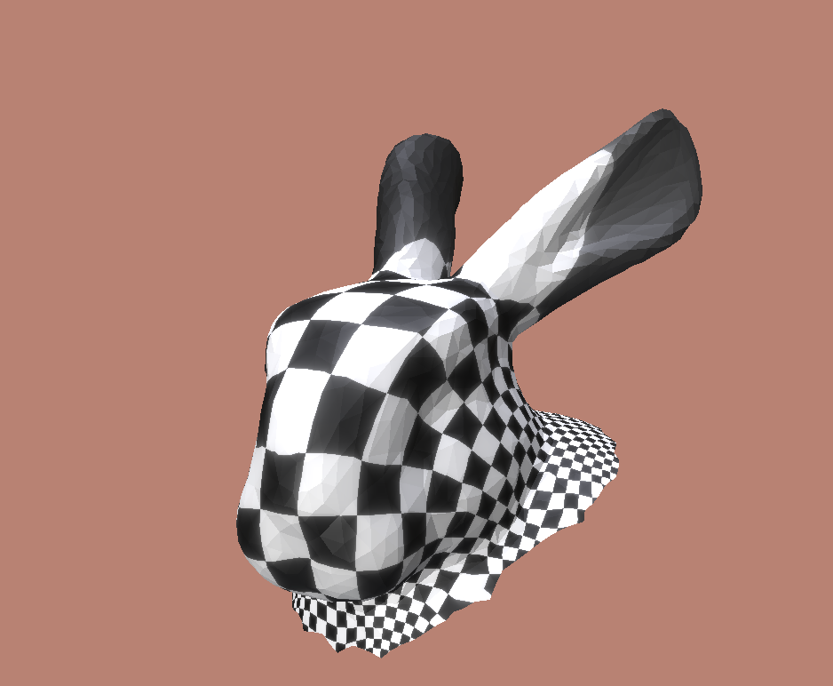
Results
Using the SCP implementation, we can now apply texturing to our open meshes as shown in the examples below.
[2] Kozłowski, W. (1992). The power method for the generalized eigenvalue problem. Roczniki Polskiego Towarzystwa Matematycznego. Seria 3, Matematyka Stosowana/Matematyka Stosowana/Mathematica Applicanda, 21(35). https://doi.org/10.14708/ma.v21i35.1790
This blog was written by Sachin Kishan and Diany Pressato during the SGI 2024 Fellowship as one of the outcomes of a two-week project under the mentorship of Ahmed Mahmoud and the support of Supriya Gadi Patil as a teaching assistant.
RXMesh is a framework for processing triangle mesh on the GPU. It allows developers to easily use the GPU’s massive parallelism to perform common geometry processing tasks. For a preliminary introduction to RXMesh, check out this tutorial blog here.
Our task was to use RXMesh to implement some classic algorithms in geometry processing. This blog details one of the algorithms we implemented: As-Rigid-As-Possible(ARAP) Surface Modeling [1].
This blog will discuss the algorithm in terms of its basic concepts, the steps of the algorithm, the implementation using RXMesh, and the final results.
Our entire implementation of ARAP deformation in RXMesh can be found here.
As-Rigid-As-Possible Surface Modeling
Sorkine and Alexa (2007) formulated a method where we can retain the shape of an object as much as possible despite deforming one (or a set of) its vertices. This retention of shape is achieved by ensuring that subsequent transformations to the mesh after deforming its vertices are rigid. This property of rigidity means that a mesh can only undergo rigid transformations such as translation or rotation, but not stretching or shearing (since these are not rigid transformations).
The algorithm’s focus is to minimize the energy which measures the extent of deformation (dubbed rigidity energy). This energy is minimized when given a specific set of positions or a specific set of rotations. Notice that we can not minimize both at once—since we need the minimized rotational transformation for minimizing the energy from deformed positions. Thus, we instead solve both alternatively, i.e., solve for deformed positions assuming rotation is fixed, then solve for rotation assuming the position is fixed.
Using a Laplacian, we can form a sparse system of linear equations which we can then solve to obtain a new set of positions for the mesh. The algorithm works as follows for a single iteration
Identify the rotation matrix for the given deformed positions which minimizes deformation energy.
Solve for the new positions to minimize the energy, given a set of linear equations.
In this case, the set of linear equations to solve is in the form :
\(Lx=b\)
Where \(L\) is the Laplace-Beltrami operator, which can be formed by finding the cotangent edge weights of the mesh, \(x\) represents the set of new vertex positions we solve for, and \(b\) represents the right-hand side of Equation 8 from Sorkine and Alexa (2007). The derivation is detailed further in the original paper.
To further minimize the energy, we can perform multiple iterations of the same steps, using updated vertex positions and consequent rotations per iteration.
Implementation
The following code snippets show how the algorithm is implemented in RXMesh.
We first deform the input mesh and set constraints on each vertex depending on whether it is fixed, deformed, or free to move. This will be taken into account when calculating the system matrix \(L\).
 // set constraints
    const vec3<float> sphere_center(0.1818329, -0.99023, 0.325066);
    rx.for_each_vertex(DEVICE, [=] __device__(const VertexHandle& vh) {
        const vec3<float> p(deformed_vertex_pos(vh, 0),
                            deformed_vertex_pos(vh, 1),
                            deformed_vertex_pos(vh, 2));

        // fix the bottom
        if (p[2] < -0.63) {
            constraints(vh) = 2;
        }

        // move the jaw
        if (glm::distance(p, sphere_center) < 0.1) {
            constraints(vh) = 1;
        }
    });
In the code above, we set the mesh to deform the dragon’s jaw and fix its bottom vertices (legs). This can vary depending on the type of input we want to have. Another possibility is to add a feature for users to click and select vertices to deform or fix them in space interactively.
Before we perform the iteration step, we calculate the Laplacian. It can be calculated as the cotangent edge weight matrix. So, we create a kernel using RXMesh.
    auto calc_mat = [&](VertexHandle v_id, VertexIterator& vv) {
        if (constraints(v_id, 0) == 0) {
            for (int i = 0; i < vv.size(); i++) {
          laplace_mat(v_id, v_id) += weight_matrix(v_id, vv[i]);
          laplace_mat(v_id, vv[i]) -= weight_matrix(v_id, vv[i]);
            }
        } else {
            for (int i = 0; i < vv.size(); i++) {
                laplace_mat(v_id, vv[i]) = 0;
            }
            laplace_mat(v_id, v_id) = 1;
        }
    };
The weight matrix is calculated using a special query called “EVDiamond”, where we obtain the two end vertices and the two opposite vertices of an edge. This gives us exactly the data we need to find the cotangent edge weight.
    auto calc_weights = [&](EdgeHandle edge_id, VertexIterator& vv) {
        // the edge goes from p-r while the q and s are the opposite vertices
        const rxmesh::VertexHandle p_id = vv[0];
        const rxmesh::VertexHandle r_id = vv[2];
        const rxmesh::VertexHandle q_id = vv[1];
        const rxmesh::VertexHandle s_id = vv[3];

        if (!p_id.is_valid() || !r_id.is_valid() || !q_id.is_valid() ||
            !s_id.is_valid()) {
            return;
        }

        const vec3<T> p(coords(p_id, 0), coords(p_id, 1), coords(p_id, 2));
        const vec3<T> r(coords(r_id, 0), coords(r_id, 1), coords(r_id, 2));
        const vec3<T> q(coords(q_id, 0), coords(q_id, 1), coords(q_id, 2));
        const vec3<T> s(coords(s_id, 0), coords(s_id, 1), coords(s_id, 2));


        T weight = 0;
   weight += dot((p - q), (r - q)) / length(cross(p - q, r - q));
   weight += dot((p - s), (r - s)) / length(cross(p - s, r - s));

        weight /= 2;
        weight = std::max(0.f, weight);

        edge_weights(p_id, r_id) = weight;
        edge_weights(r_id, p_id) = weight;
    };
We now have all the building blocks necessary to perform an iteration step. This is what an iteration loop looks like:
    // process step
    for (int i = 0; i < iterations; i++) {
        // solver for rotation
        calculate_rotation_matrix<float, CUDABlockSize>
            <<<lb_rot.blocks, lb_rot.num_threads, lb_rot.smem_bytes_dyn>>>(
                rx.get_context(),
                ref_vertex_pos,
                deformed_vertex_pos,
                rotations,
                weight_matrix);

        // solve for position
        calculate_b<float, CUDABlockSize>
            <<<lb_b_mat.blocks,
               lb_b_mat.num_threads,
               lb_b_mat.smem_bytes_dyn>>>(rx.get_context(),
                                          ref_vertex_pos,
                                          deformed_vertex_pos,
                                          rotations,
                                          weight_matrix,
                                          b_mat,
                                          constraints);

        laplace_mat.solve(b_mat, *deformed_vertex_pos_mat);
    }
We perform multiple iterations of the algorithm to effectively minimize the energy. We can see in the code above that we alternatively solve for rotation and then for positions. We first calculate the rotation matrix given a set of deformed positions, then calculate the \(b\) matrix (as defined earlier) and then solve the system of equations to identify the new vertex positions.
The following kernel calculates the rotation matrix per vertex to minimize the rigidity energy given their positions.
auto cal_rot = [&](VertexHandle v_id, VertexIterator& vv) {
        Eigen::Matrix3f S = Eigen::Matrix3f::Zero();

        for (int j = 0; j < vv.size(); j++) {

            float w = weight_matrix(v_id, vv[j]);

            Eigen::Vector<float, 3> pi_vector = {
              ref_vertex_pos(v_id, 0) - ref_vertex_pos(vv[j], 0),
              ref_vertex_pos(v_id, 1) - ref_vertex_pos(vv[j], 1),
              ref_vertex_pos(v_id, 2) - ref_vertex_pos(vv[j], 2)
};


            Eigen::Vector<float, 3> pi_dash_vector = {
                deformed_vertex_pos(v_id, 0) - deformed_vertex_pos(vv[j], 0),
                deformed_vertex_pos(v_id, 1) - deformed_vertex_pos(vv[j], 1),
                deformed_vertex_pos(v_id, 2) - deformed_vertex_pos(vv[j], 2)};

            S = S + w * pi_vector * pi_dash_vector.transpose();
        }

        Eigen::Matrix3f U;         // left singular vectors
        Eigen::Matrix3f V;         // right singular vectors
        Eigen::Vector3f sing_val;  // singular values

        svd(S, U, sing_val, V);

        const float smallest_singular_value = sing_val.minCoeff();


        Eigen::Matrix3f R = V * U.transpose();

        if (R.determinant() < 0) {
            U.col(smallest_singular_value) =
                U.col(smallest_singular_value) * -1;
            R = V * U.transpose();
        }

        // Matrix R to vector attribute R

        for (int i = 0; i < 3; i++)
            for (int j = 0; j < 3; j++)
                rotations(v_id, i * 3 + j) = R(i, j);
    };
We first find the Single Value Decomposition (SVD) of the sum (\(S_{i} \)) where
\(S_{i}=\sum_{j\in N(i)} w_{ij}e_{ij}e^{‘T}_{ij} \) (Equation 5 in Sorkine and Alexa(2007))
We then use that to calculate rotation and assign that as the vertice’s rotation. After we calculate rotation, we calculate the right-hand side of Equation 8 as stated earlier.
auto init_lambda = [&](VertexHandle v_id, VertexIterator& vv) {
        // variable to store ith entry of b_mat
        Eigen::Vector3f bi(0.0f, 0.0f, 0.0f);

        // get rotation matrix for ith vertex
        Eigen::Matrix3f Ri = Eigen::Matrix3f::Zero(3, 3);

        for (int i = 0; i < 3; i++) {
            for (int j = 0; j < 3; j++)
                Ri(i, j) = rotations(v_id, i * 3 + j);
        }

        for (int nei_index = 0; nei_index < vv.size(); nei_index++) {
            // get rotation matrix for neightbor j
            Eigen::Matrix3f Rj = Eigen::Matrix3f::Zero(3, 3);
            for (int i = 0; i < 3; i++)
                for (int j = 0; j < 3; j++)
                    Rj(i, j) = rotations(vv[nei_index], i * 3 + j);

            // find rotation addition
            Eigen::Matrix3f rot_add = Ri + Rj;
            // find coord difference
            Eigen::Vector3f vert_diff = {
                ref_vertex_pos(v_id, 0) - ref_vertex_pos(vv[nei_index], 0),
                ref_vertex_pos(v_id, 1) - ref_vertex_pos(vv[nei_index], 1),
                ref_vertex_pos(v_id, 2) - ref_vertex_pos(vv[nei_index], 2)};

            // update bi
            bi = bi +
                 0.5 * weight_mat(v_id, vv[nei_index]) * rot_add * vert_diff;
        }

        if (constraints(v_id, 0) == 0) {
            b_mat(v_id, 0) = bi[0];
            b_mat(v_id, 1) = bi[1];
            b_mat(v_id, 2) = bi[2];
        } else {
            b_mat(v_id, 0) = deformed_vertex_pos(v_id, 0);
            b_mat(v_id, 1) = deformed_vertex_pos(v_id, 1);
            b_mat(v_id, 2) = deformed_vertex_pos(v_id, 2);
        }
    };
After calling both these kernels, we use the solve function to solve the equations. We then update the mesh with this new set of vertex positions.
Results
Using the implementation above, we can create a per-frame ARAP implementation to animate movement for a mesh. In the example below, we fix the upper half vertices of Spot the Cow and allow the bottom half to freely deform. We then move each of the bottom “feet” vertices in every frame to animate a swimming or walking-like movement in Spot.
The bottom feet vertices are user-deformed , the upper vertices are fixed, and the bottom half (except the feet) are free to move—and are determined by the ARAP algorithm.
Here’s another example with the dragon mesh.
Deform a vertex of the dragon’s jaw while keeping its feet fixed.
Further work
Polyscope shows us that the framerate of these demos is very poor (below 30 fps). We would expect it to do better, especially when using the GPU. A performance analysis as well as optimizing of the solver will be required to make the application reach desired levels of real-time processing.
References
[1] Olga Sorkine and Marc Alexa. 2007. As-rigid-as-possible surface modeling. In Proceedings of the fifth Eurographics symposium on Geometry processing (SGP ’07). Eurographics Association, Goslar, DEU, 109–116. https://doi.org/10.2312/SGP/SGP07/109-116
This blog was written by Sachin Kishan during the SGI 2024 Fellowship as one of the outcomes of a two-week project under the mentorship of Ahmed Mahmoud and the support of Supriya Gadi Patil as a teaching assistant.
SGI Fellows: Harini Rammohan, Nicolas Pigadas, Riccardo Ali
Project Mentors: Mahdi Saleh and Dani Velikova
SGI Volunteer: Matheus Araujo
Optimal Transport and the Sinkhorn Algorithm:
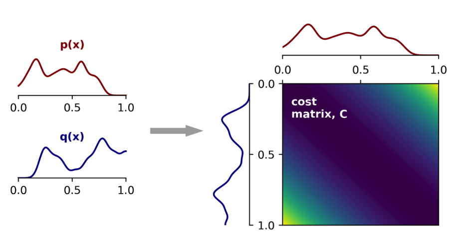
Optimal Transport (OT), intuitively speaking, finds the most efficient way to transport mass from one probability distribution to another. For example, suppose the surface of a beach is given as the ambient space \(X\), and the various distributions of sand on the surface are represented by probability distributions on \(X\). Suppose also that we are given a cost function \(C:X\times X\to\mathbb{R}_{\geq 0} \), where \(C(x,y)\) represents the cost of moving a unit mass of sand from point \(x\) to point \(y\). The OT problem in this setting is to move the sand from a source distribution to a target distribution while minimizing the total transportation cost. Working with continuous distributions is often not feasible computationally, so a common approach is to discretize distributions, say by dividing the beach into a finite collection of bins and extracting an optimal transport plan for moving sand amongst this finite collection.
In the discrete case, the transportation cost can represented by a cost matrix \(C\), where \(C_{i,j}\) is the cost of moving a unit mass of sand from bin \(i\) to bin \(j\). The Wasserstein distance between two distributions is defined as the transportation cost for the minimal transport plan and can be obtained via the Sinkhorn Algorithm. Sinkhorn’s theorem states that if \(A\) is a square matrix with positive entries, then there exist two diagonal matrices \(D_1\) and \(D_2\) with positive diagonal entries such that \(T = D_1AD_2\) is doubly stochastic (all rows and columns sum to 1). The algorithm recursively rescales rows and columns of the input matrix A until it converges to the required matrix \(T\). \(T_{ij}\) returns the amount of mass that must be transported from bin \(i\) to bin \(j\) in the minimal transport plan.
Representation of the cost matrix for the 1D problem Image from https://alexhwilliams.info/itsneuronalblog/2020/10/09/optimal-transport/
6D Pose Estimation using the Sinkhorn Solver:
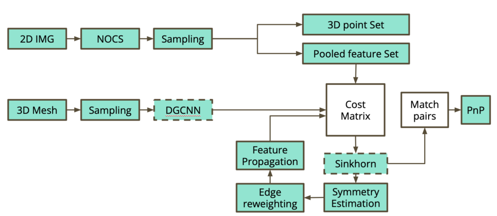
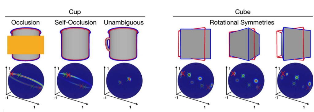
6D pose estimation refers to the process of determining the position and orientation (together called the pose) of an object (CAD) in a three-dimensional space from an image of that object. Seeing pixels as bins and pixel values as the mass of sand in that bin, the Sinkhorn algorithm can be used to find a transport plan for matching pixels in the image to points in \(\mathbb{R}^3\). However, if the object is symmetric, there may be ambiguity in its pose and one could get multiple poses that match the image. In this case, the standard Sinkhorn approach fails. Inspired by the work in the SuperGlue {1} and EPOS {2} papers, we aimed to extend the differentiable Sinkhorn solver to cases with one-to-many solutions and incorporate graph neural networks to estimate the 6D pose of such symmetric objects.
The proposed pipeline for the project
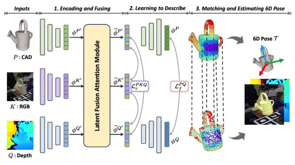
6D Object Pose Estimation Image from Huang, Junwen, et al. “Matchu: Matching unseen objects for 6d pose estimation from rgb-d images.”CVPR. 2024
The hurdles were, first to come up with a cost matrix that best suited the problem, implement a one-to-many Sinkhorn solver from the Python OT library, and use a Perspective-N-Point {5} approach to find the pose of each of the solutions returned by the Sinkhorn solver. Another challenge was finding the correct axis of symmetry of the pose; we planned to first assume prior information about the axis of symmetry and later incorporate the problem of finding this axis itself. Unfortunately, we decided not to continue with the second week of the project and hence were not able to produce concrete results. However, a brief description of our ideas for overcoming each hurdle is given below.
Ambiguity due to symmetry Image from Manhardt, Fabian, et al. “Explaining the ambiguity of object detection and 6d pose from visual data.” ICCV 2019.
Ideas for the Implementation:
The image was meant to be a 2D point cloud with features from which we could determine a partial 3D point cloud. One idea we had for the cost matrix, in the case where the axis of symmetry is known, was to add a symmetry-aware cost to reduce the cost for matches that are consistent with the given symmetry. We could also try to find the translation vector by inferring it from points on the axis of symmetry of the CAD and the corresponding matches in the image. Once we do this, we will have to deal with the rotation vector, which can be optimized separately using the Sinkhorn algorithm.
The special Euclidean group (SE(3)) is the group of all combinations of rotations, reflections, and translations in \(\mathbb{R}^3\). If we have no information about the axis of symmetry, then this group forms the set of all possible 6D poses. In this case, we must find poses in SE(3) that minimize transportation costs. We could try to compare images of the CAD after applying a pose and the 2D image point cloud and reduce the distance between the two to find the possible poses of the image.
One approach to extend the existing Sinkhorn solver to get multiple solutions is first to use the existing one to get a single solution, and then find all transport matrices that have a similar cost to the one obtained. Another is to design a collection of cost matrices rather than a single one, in a way that the existing Sinkhorn solver produces multiple (and hopefully all) possible solutions. We could get this collection of matrices by applying various poses to the original CAD as before and compute the cost of going from the modified CADs to the image.
Acknowledgements:
During the one week of the project, I learned so much about optimal transport, image matching, and pose estimation. I am very grateful to our mentors who supported and guided our progress.
This blog post is a follow up to “How to match the “wiggliness” of two shapes”, where we discussed the metrics we use to measure the similarity between two surfaces. In that post, we briefly talked about approximating a surface by using a regular grid to generate vertices for an approximation mesh. There we observed that as we increased the number of vertices, the surface approximation error decreases. This is somewhat intuitive – as you increase the “fineness” of the approximation mesh, the more closely you would expect it to approximate the actual surface. However, in practical applications we aim to keep the number of vertices as low as possible, in order to reduce both memory space and the amount of runtime computation.
So what can we do to improve the surface approximation without increasing the number of vertices? Are there better ways to select vertices – such that we can minimize the chamfer distance error? This is what we will be exploring in this post.
Regular grids
Before we try different ways of selecting vertex positions. Hence we repeat the same experiment with a few different surfaces, using a regular grid to generate mesh vertices. First we start with three basic cases with different gaussian curvatures:
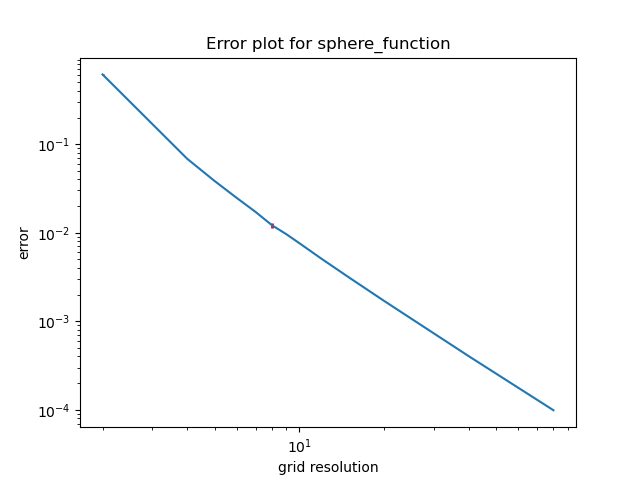
Sphere function (positive gaussian curvature)
Figure 1. Sphere function approximated with regular grid vertices.Figure 2. Log-log error plot of grid vertices dimensions and chamfer distance error for the sphere function
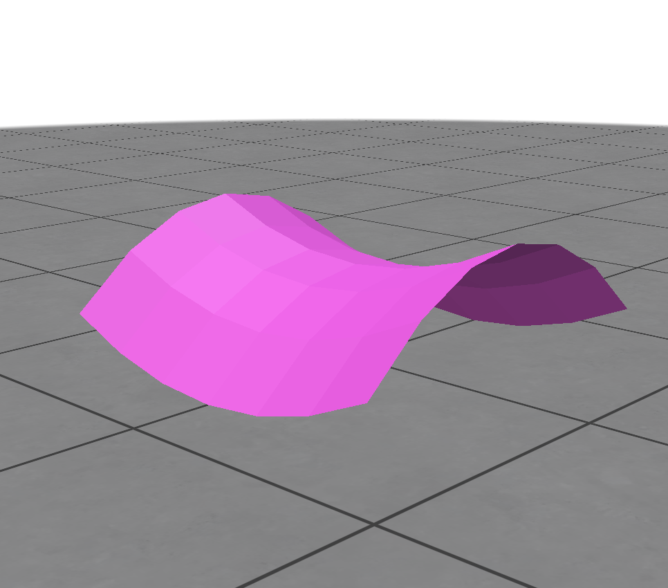
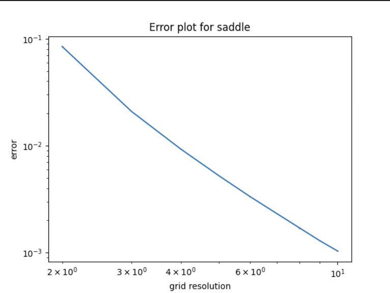
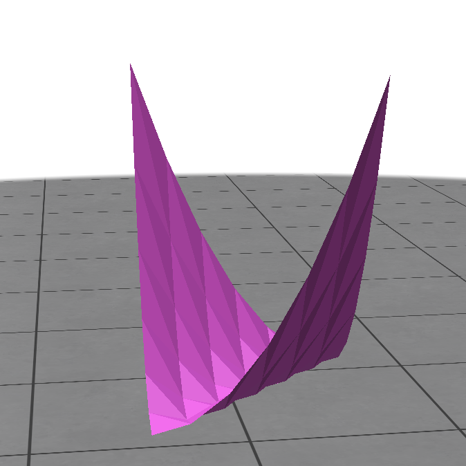
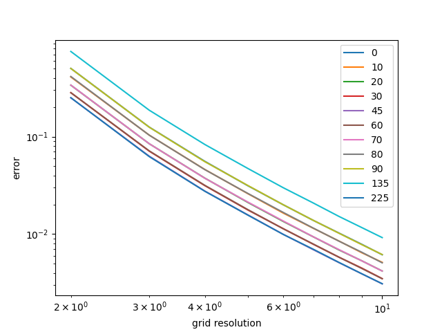
2. Saddle function (negative gaussian curvature)
Figure 3. Saddle function approximated with regular grid vertices.Figure 4. Log-log error plot of grid vertices dimensions and chamfer distance error for the saddle function
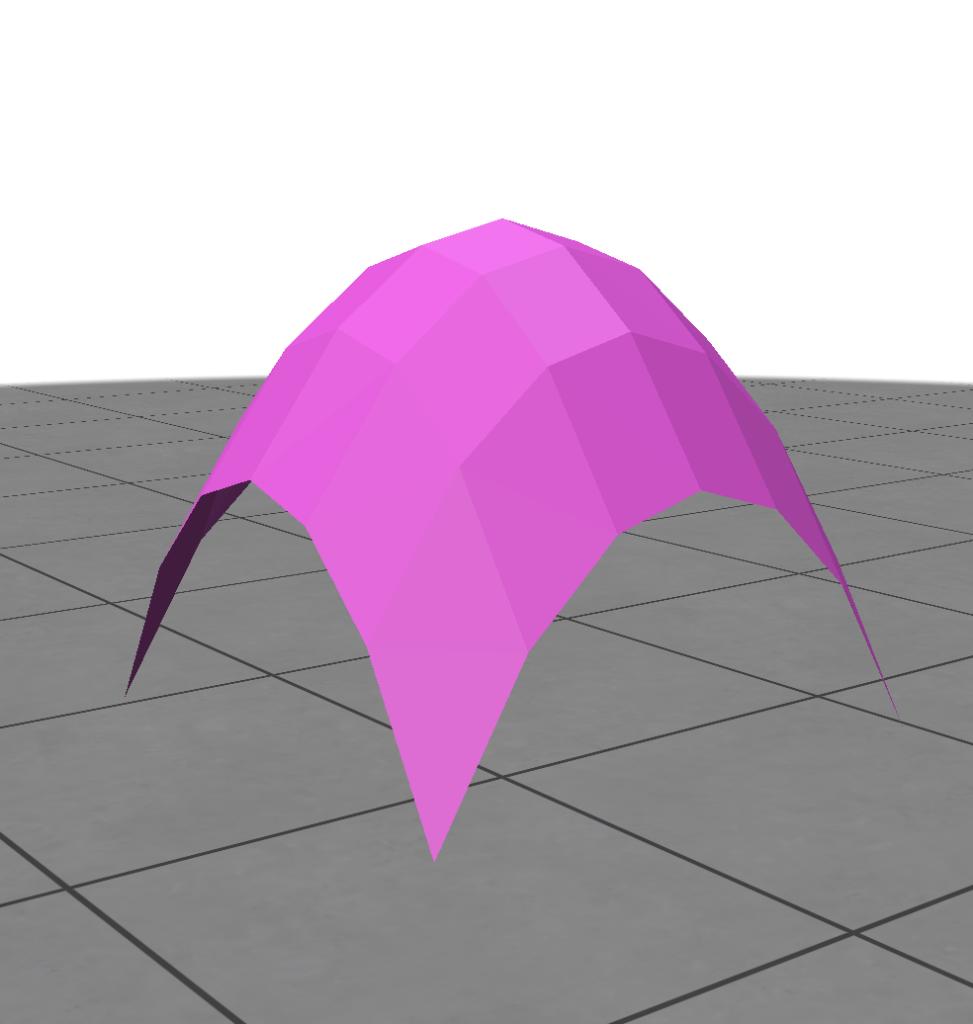
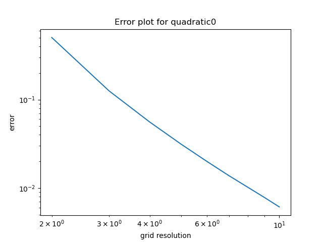
3. Quadratic function (0 gaussian curvature)
Figure 5. Quadratic function approximated with regular grid vertices.Figure 6. Log-log error plot of grid vertices dimensions and chamfer distance error for the quadratic function
So far everything works well similarly to the previous blog post – the error decreases consistently as the grid resolution.
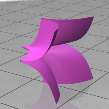
In order to really visualize the limitations of using the regular grid to sample points on the mesh, we decided to also include a more “extreme” function that looks harder to approximate – the Cross-in-tray function, which has a few asymptotes.
4. Cross-in-tray function
Figure 7. Cross-in-tray function approximated with regular grid vertices
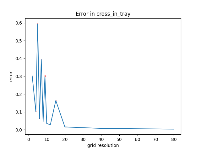
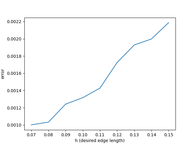
For this function, we noticed something unusual. When we increase the grid resolution from 6×6, to 7×7, to 8×8, we notice a sharp increase, then decrease in error, unlike the consistent decrease in error as we saw before.
Figure 8. Error plot of grid vertices dimensions and chamfer distance error for the quadratic function
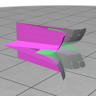
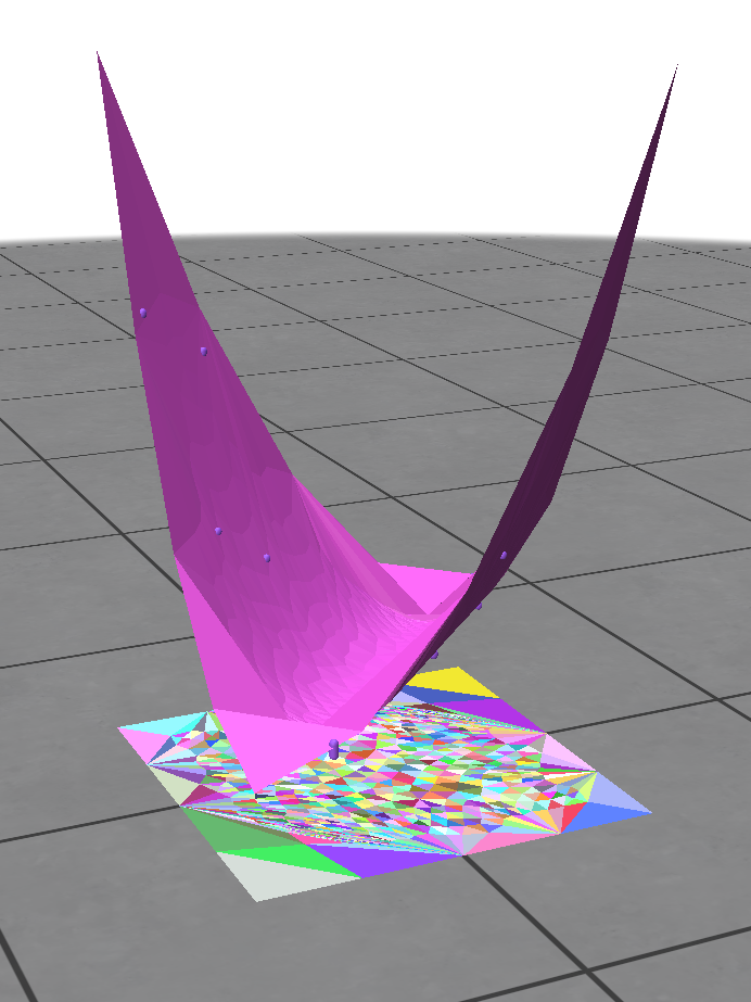
We decided to visualize what might be causing this in the figures 9-11 below, where the green transparent surface represents a close approximation of the actual surface, and the magenta surface shows the surface generated by sampling the regular grids with the different dimensions mentioned .
Figure 9. Approximation with 6×6 grid verticesFigure 10. Approximation with 7×7 grid verticesFigure 11. Approximation with 8×8 grid vertices
As seem above, the increase in the approximation error for the 7×7 regular grid is caused by the alignment of the selected vertices with the planes that the asymptotes lie on.
This is an interesting observation, as we can visibly see that the alignment of the vertices to certain features or properties of a surface affects the surface approximation error. There have been works [1][2] that have touched on heuristics about how when the mesh edges are orthogonal to the direction of principal curvature of the original function it often (but not always!) results in a lower approximation error. The next two type of experiments look into this further.
Rotated surface function
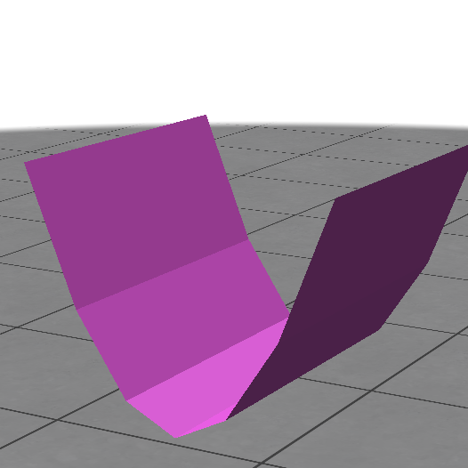
We decided to test the alignment of the edges to the direction of principal curvature on the quadratic function, as we could easily identify this direction for this function. We rotated the surface by different angles and generated approximations using the same regular grid, then plotted its error.
Figure 12. Approximation of unrotated quadratic functionFigure 13. Approximation of quadratic function rotated 45 degrees around the z axis
Interestingly, the error is the lowest when the quadratic function is rotated 45 degrees and 225 degrees and highest. This is notable because when the function is rotated 0 or 90 degrees, the short edges of the triangles are in fact orthogonal to the direction of principal curvature, so according to the heuristic these cases should have given the lowest error.
After closer observation we realized that the 45 degrees and 225 degrees cases are when the longest edge of the triangles are orthogonal with the curvature of the quadratic surface. Perhaps more work can be done to look into this in the future!
Re-meshed grid
We also use the Botsch-Kebbelt re-meshing algorithm to re-mesh the regular grid, to generate more randomness in the alignment of the triangles to the principal curvature of the quadratic function. This algorithm takes in the surface as well as the desired average edge lengths of the the triangles in the mesh, and outputs to us a re-meshed surface. The images from left to right demonstrates what happens as we increase the average edge length that we pass in as a parameter.
Figure 15. Approximation of surface using a re-meshed grid with 0.15 desired edge lengthFigure 16. Approximation of surface using a re-meshed grid with 0.07 desired edge length
Figure 17. Error plot of input desired re-meshed edge length and chamfer distance error
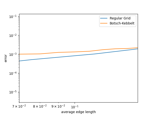
To make a more equal comparison, we converted the grid resolution to find the average edge length of the triangles in the regular grids and plotted its error together on a log-log graph. As we can see below, the regular grid does better than the Bosch-Kebbelt re-meshed grid. This is congruent with what we expected – that aligning the edges of the triangles would give us a lower error than just random orientations!
Figure 18. Comparison of the chamfer distance error for the regular grid and the botsch-kebbelt re-meshed grid
References:
[1] Bommes, David, et al. “Mixed-integer quadrangulation.” ACM Transactions on Graphics, vol. 28, no. 3, July 2009, pp. 1–10, doi:10.1145/1531326.1531383.
[2] Jakob, Wenzel, et al. “Instant Field-aligned Meshes.” ACM Transactions on Graphics, vol. 34, no. 6, Nov. 2015, pp. 1–15, doi:10.1145/2816795.2818078.
TetSphere Splatting [Guo et al., 2024] is a cutting-edge technique for high-quality 3D shape reconstruction using tetrahedral meshes. This method stands out by delivering superior geometry without relying on neural networks or post-processing. Unlike traditional Eulerian methods, TetSphere Splatting excels in applications such as single-view 3D reconstruction and text-to-3D generation.
Our project aimed to enhance TetSphere Splatting through two key improvements:
Geometry Optimization: We integrated subdivision and remeshing techniques to refine the geometry optimization process, enabling the capture of finer details and better tessellation.
Adaptive TetSphere Modification: We developed adaptive mechanisms for splitting and merging tetrahedral spheres, enhancing flexibility and detail in the optimization process.
Setting up the Code Base:
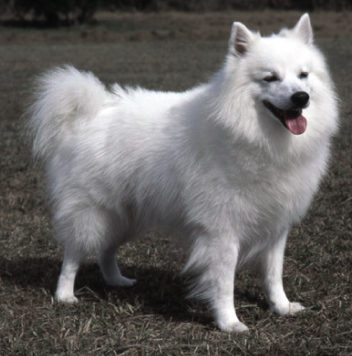
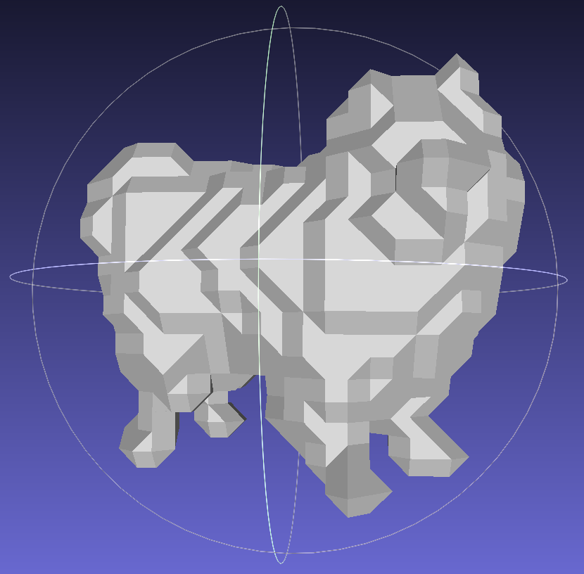
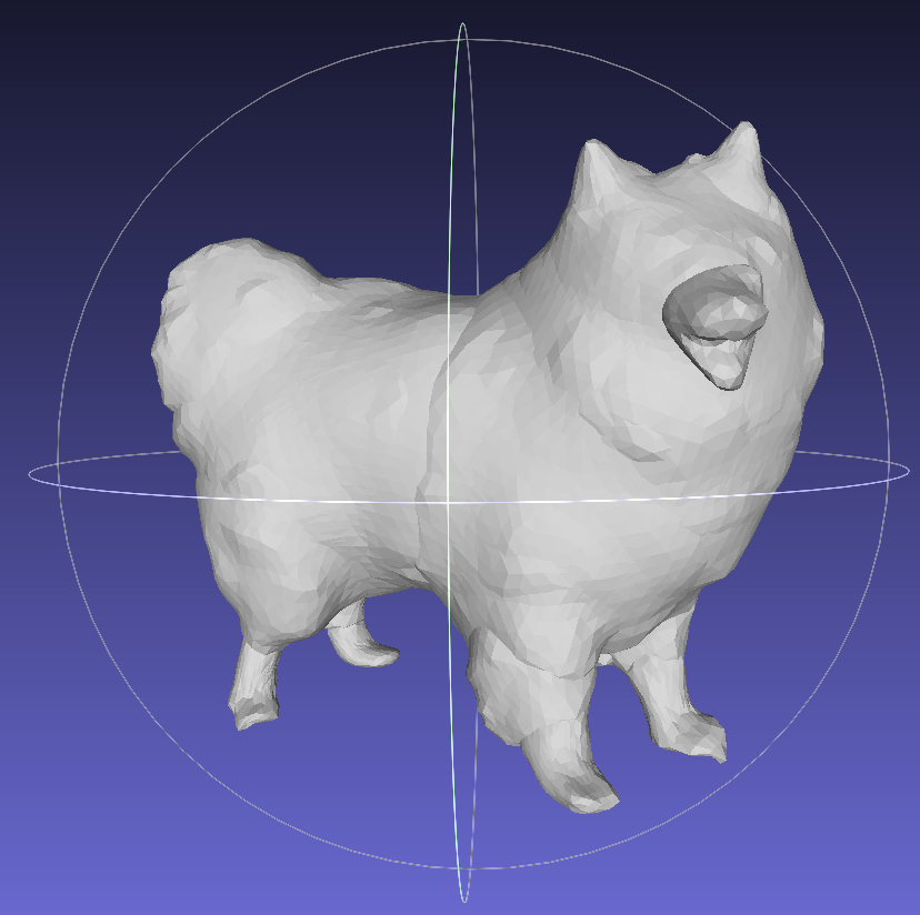
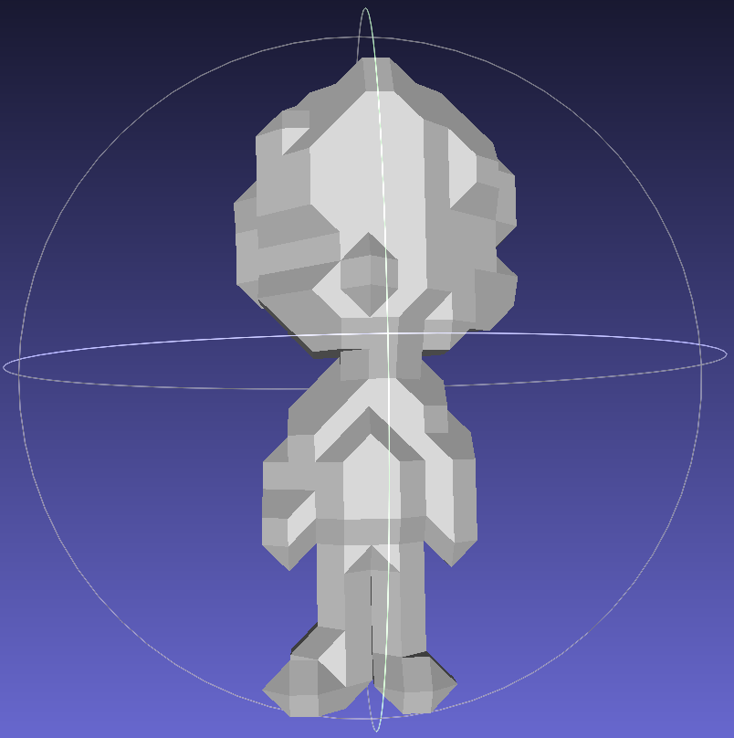
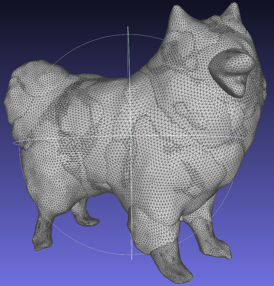
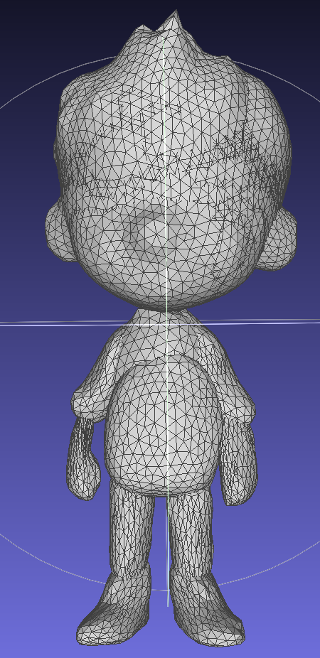
Our mentor, Minghao, facilitated the setup of the codebase in a cloud environment equipped with GPU support. Using a VSCode tunnel, we were able to work remotely and make modifications within the same environment. Following the instructions in the TetSphere Splatting GitHub README file, we successfully initialized the TetSpheres and executed the TetSphere Splatting process for our input images, including those of a white dog and a cartoon boy.
Input Image of a White DogTetSphere InitializationTetsphere SplattingInput Image of a Cartoon BoyTetsphere InitializationTetsphere Splatting
Geometry Optimization:
To improve the geometry optimization in TetSphere Splatting, we explored various algorithms for adaptive remeshing and subdivision. Initially, we considered parametrization-based remeshing using Centroidal Voronoi Tessellation (CVT) but opted for direct surface remeshing due to its efficiency and simplicity. For subdivision, we chose the Loop subdivision algorithm, as it is specifically designed for triangle meshes and better suited for our application compared to Catmull-Clark.
Implementing Loop Subdivision:
In the second week of the project, I worked on implementing the loop subdivision algorithm and incorporating it into the Geometry Optimization pipeline. Below is a detailed explanation of the algorithm and the method of implementation using the example of the example of the white dog mesh after TetSphere splatting.
1. Importing the required libraries, loading and initializing the mesh:
Instead of working throughout with numpy arrays, I chose to use defaultdict, a subclass of Python dictionaries to reduce the running time of the program. unique_edges defined below ensures that the list of edges doesn’t count each edge twice, once as (e1, e2) and once as (e2, e1).
import trimesh
import numpy as np
from collections import defaultdict

init_mesh = trimesh.load("./results/a_white_dog/final/final_surface_mesh.obj")
V = init_mesh.vertices
F = init_mesh.faces
E = init_mesh.edges

def unique_edges(edges):
    sorted_edges = np.sort(edges, axis=1)
    unique_edges = np.unique(sorted_edges, axis=0)
    return unique_edges
2. Edge-Face Adjacency Mapping
This maps edges to the faces they belong to, which will later help to identify boundary and interior edges.
def compute_edge_face_adjacency(faces):
    edge_face_map = defaultdict(list)
    for i, face in enumerate(faces):
        v0, v1, v2 = face
        edges = [(min(v0, v1), max(v0, v1)),
                 (min(v1, v2), max(v1, v2)),
                 (min(v2, v0), max(v2, v0))]
        for edge in edges:
            edge_face_map[edge].append(i)
    return edge_face_map
3. Computing New Vertices:
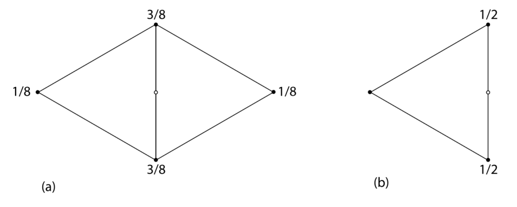
If an edge is a boundary edge (it belongs to only one face), then the new vertex is simply the midpoint of the two vertices at the ends of the edge. If not, the edge belongs to two faces and the new vertex is found to be a weighted average of the four vertices which make the two faces, with a weight of 3/8 for the vertices on the edge and 1/8 for the vertices not on the edge. The function also produces indices for the new vertices.
def compute_new_vertices(edge_face_map, vertices, faces):
    new_vertices = defaultdict(list)
    i = vertices.shape[0] - 1
    for edge, facess in edge_face_map.items():
        v0, v1 = edge
        if len(facess) == 1:  # Boundary edge
            i += 1
            new_vertices[edge].append(((vertices[v0] + vertices[v1]) / 2, i))
        elif len(facess) == 2:  # Internal edge
            i += 1
            adjacent_vertices = []
            for face_index in facess:
                face = faces[face_index]
                for vertex in face:
                    if vertex != v0 and vertex != v1:
                        adjacent_vertices.append(vertex)
            v2 = adjacent_vertices[0]
            v3 = adjacent_vertices[1]
            new_vertices[edge].append(((1 / 8) * (vertices[v2] + vertices[v3]) +
                                       (3 / 8) * (vertices[v0] + vertices[v1]), i))
    return new_vertices
4. Create a dictionary of updated vertices:
This generates updated vertices that include both old and newly created vertices.
def generate_updated_vertices(new_vertices, vertices, edges):
    updated_vertices = defaultdict(list)
    for i in range(vertices.shape[0]):
        vertex = vertices[i, :]
        updated_vertices[i].append(vertex)
    for i in range(edges.shape[0]):
        e1, e2 = edges[i, :]
        edge = (min(e1, e2), max(e1, e2))
        vertex, index = new_vertices[edge][0]
        updated_vertices[index].append(vertex)
    return updated_vertices
5. Construct New Faces:
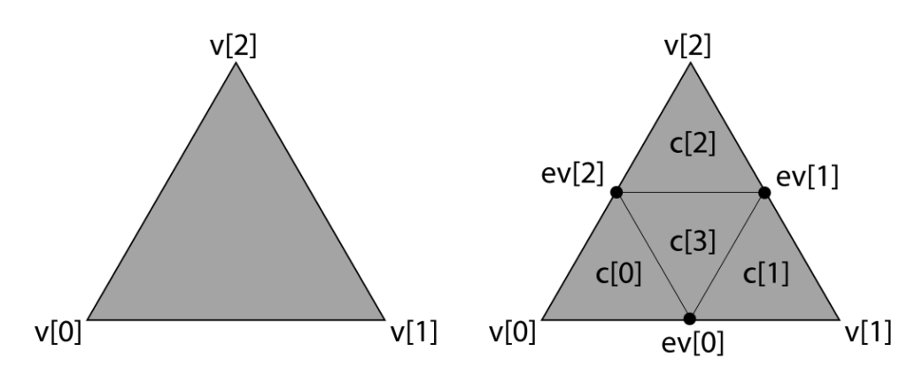
This constructs new faces using the updated vertices. Each old face is split into four new faces.
The four child faces created, ordered such that the ith child face is adjacent to the ith vertex of the original face and the fourth child face is in the center of the subdivided face. Image from https://www.pbr-book.org/3ed-2018/Shapes/Subdivision_Surfaces
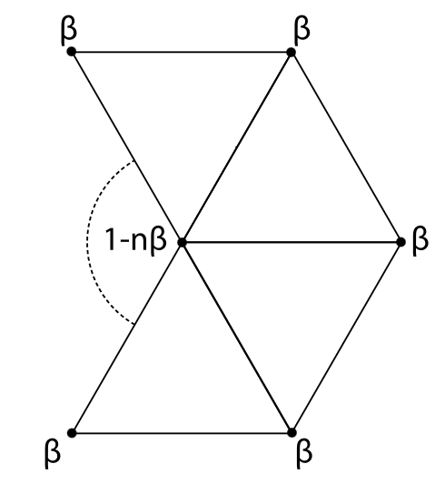
First, the function compute_vertex_adjacency finds the neighbors of each vertex. Then modify_vertices weights each of the neighbor vertices of each old vertex by a weight β (defined in the code below) and weights the old vertex by 1-nβ, where n is the degree of the old vertex. It does not change the new vertices.
def compute_vertex_adjacency(faces):
    vertex_adj_map = defaultdict(set)
    for face in faces:
        v0, v1, v2 = face
        vertex_adj_map[v0].add(v1)
        vertex_adj_map[v0].add(v2)
        vertex_adj_map[v1].add(v0)
        vertex_adj_map[v1].add(v2)
        vertex_adj_map[v2].add(v0)
        vertex_adj_map[v2].add(v1)
    return vertex_adj_map

def modify_vertices(vertices, updated_vertices, vertex_adj_map):
    modified_vertices = defaultdict(list)
    for i in range(len(updated_vertices)):
        if i in range(vertices.shape[0]):
            vertex = vertices[i,:]
            neighbors = vertex_adj_map[i]
            n = len(neighbors)
            beta = (5 / 8 - (3 / 8 + 1 / 4 * np.cos(2 * np.pi / n)) ** 2)/n
            weight_v = 1 - beta * n
            modified_vertex = weight_v * vertex
            for neighbor in neighbors:
                neighbor_point = updated_vertices[neighbor][0]
                modified_vertex += beta * neighbor_point
            modified_vertices[i].append(modified_vertex)
        else:
            modified_vertices[i].append(updated_vertices[i][0])
    return modified_vertices
7. Generating the Final Subdivided Mesh:
Now, all that is left is to collect the modified vertices and faces as numpy arrays and create the final subdivided mesh. The function loop_subdivision_iter simply applies the loop subdivision iteratively ‘n’ times, further refining the loop each time.
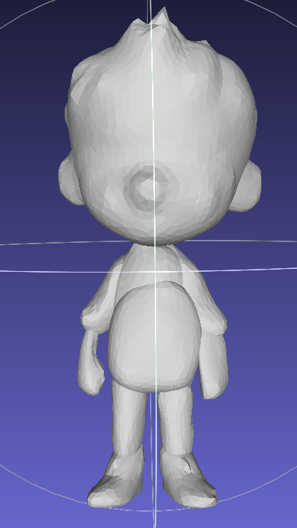
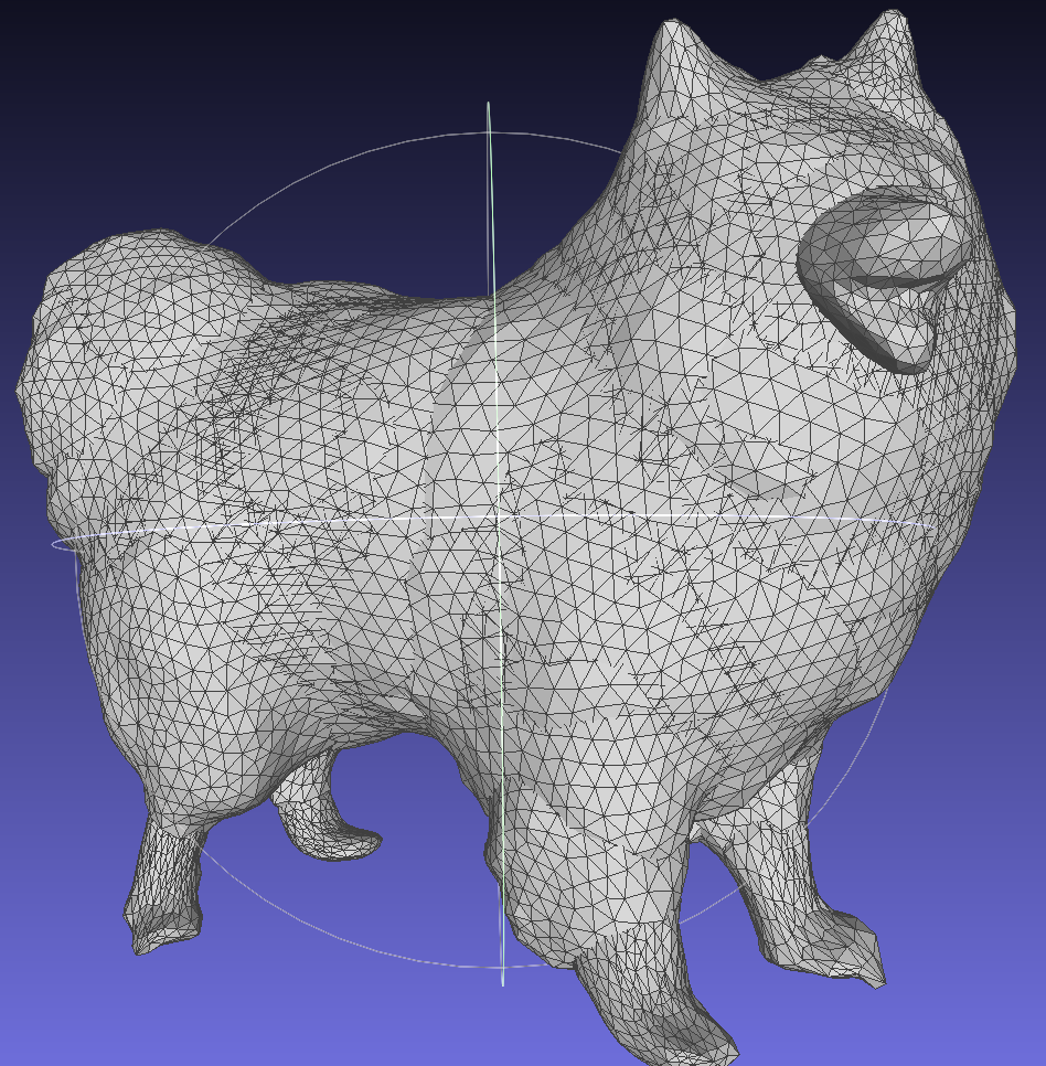
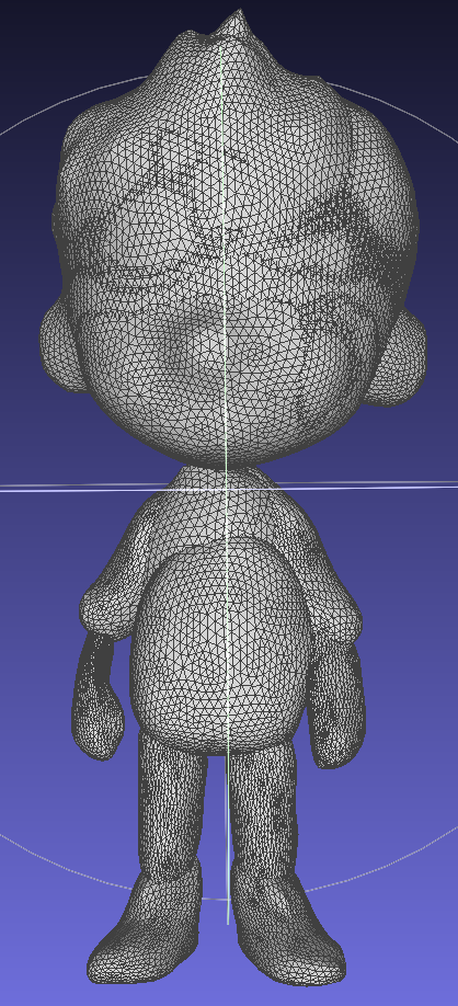
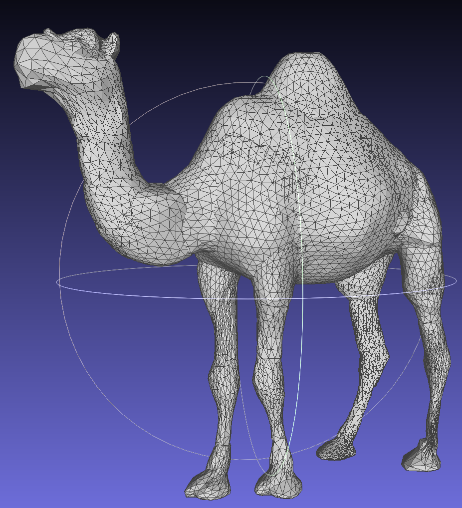
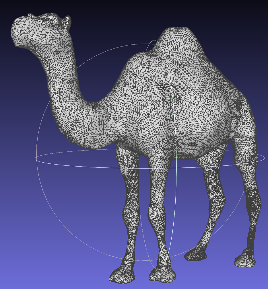
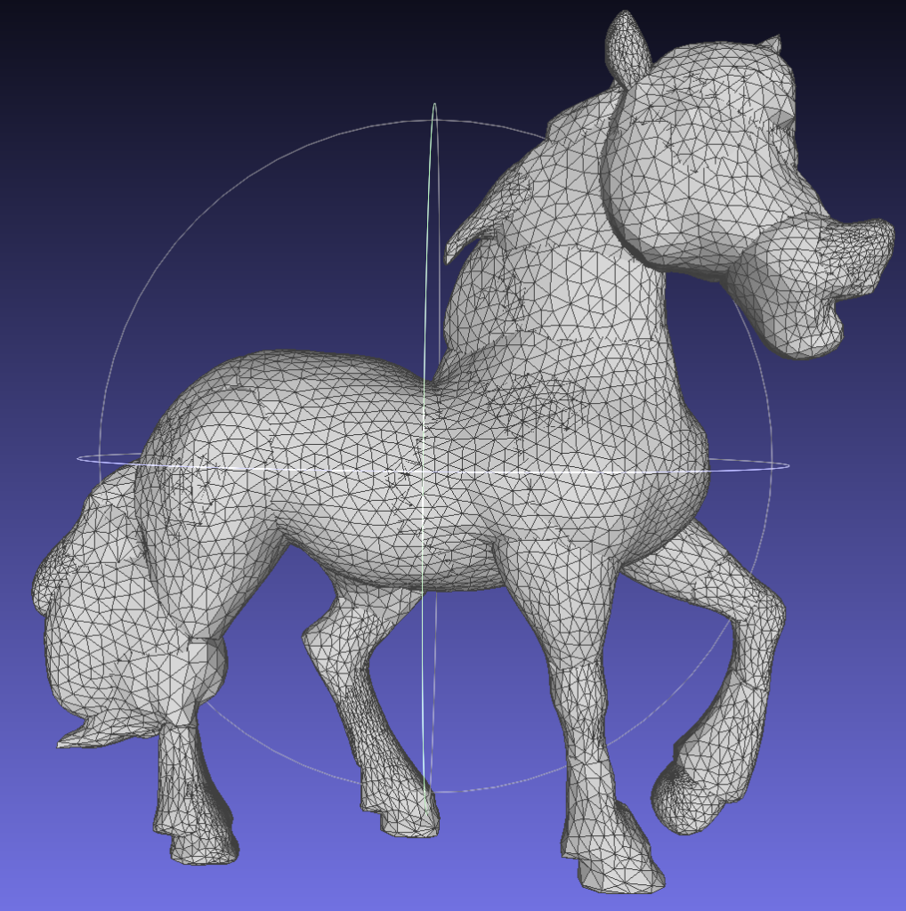
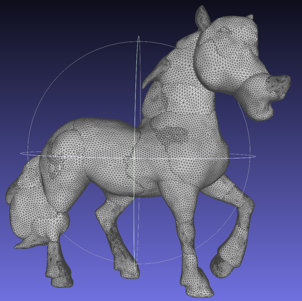
I used the above code to obtain the subdivided meshes for four input meshes – a white dog, a cartoon boy, a camel, and a horse. The results for each of these are displayed below.
Subdivision of the white dog meshSubdivision of the cartoon boy meshSubdivision of the camel meshSubdivision of the horse mesh
Conclusion:
The project successfully enhanced the TetSphere Splatting method through geometry optimization and adaptive TetSphere modification. The implementation of Loop subdivision refined mesh detail and smoothness, as evidenced by the improved results for the test meshes. The adaptive mechanisms introduced greater flexibility, contributing to more precise and detailed 3D reconstructions.
Through this project I learned a lot about TetSphere Splatting, Geometry Optimization and Loop Subdivion. I am very grateful to Minghao and Shanthika who supported and guided us in our progress.
During these six fascinating weeks at SGI, I have said and heard the words “bug” and “debugging” so often that if I had an inch for every time, I could go from Egypt to Tahiti and back a few dozen times. Haha! As an etymology enthusiast, I couldn’t resist digging into the origins of these terms. Here’s what I discovered.
The use of the term “bug” in engineering and technology contexts dates back to at least the 19th century. The term was used by Thomas Edison in a letter written in 1878 to Tivadar Puskás here, in which Edison referred to minor engineering flaws or difficulties as “bugs,” implying that these small issues were natural in the process of invention and experimentation.
Specifically, Edison wrote about the challenges of refining his inventions in this letter, stating:
“It has been just so in all of my inventions. The first step is an intuition—and comes with a burst, then difficulties arise—this thing gives out and [it is] then that ‘bugs’—as such little faults and difficulties are called—show themselves, and months of intense watching, study and labor are requisite before commercial success—or failure—is certainly reached.”
Thomas Edison and His ‘Insomnia Squad’: Debugging Inventions All Night and Napping Through the Day. Photo: Bettmann/Getty Images
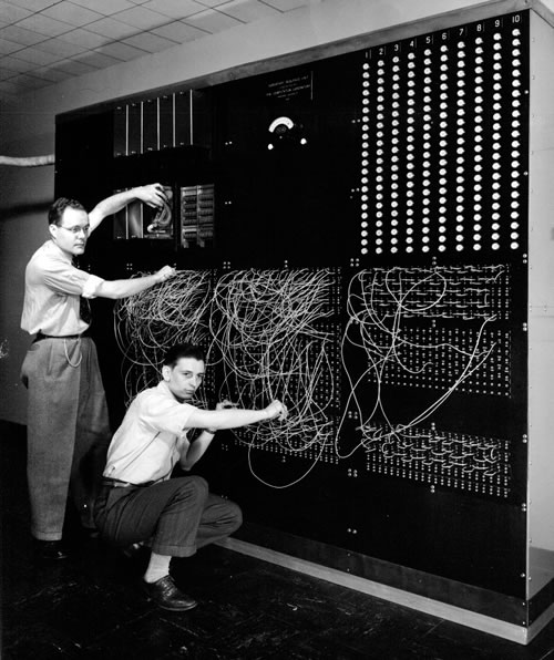
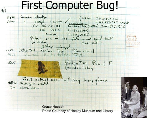
The term gained further prominence in the mid-20th century, especially in computing when engineers working on the Mark II computer at Harvard University in 1947, and found that the computer was malfunctioning. Upon investigation, Grace Hopper discovered that a moth had become trapped in one of the machine’s relays (Relay #70 on Panel “F” of the Harvard Mark II Aiken Relay Calculator), causing a problem, and took a photo of it and documented it.
Harvard Mark II Aiken Relay Calculator
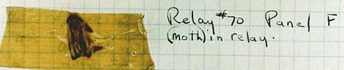
The engineers removed the moth and taped it into the log book with the note: “First actual case of a bug being found.” While the term “bug” had already been in use to describe technical issues or glitches, this incident provided a literal example of the term, and it is often credited with popularizing the concept of “de-bugging” in computer science.
The logbook, complete with the taped moth, is preserved in the Smithsonian National Museum of American History as a notable piece of computing history. This incident symbolically linked the term “bug” with computer errors in popular culture and the history of technology.
Turns out that the term “bug” has a rich etymology, originating in Middle English where it referred to a ghost or hobgoblin that troubled and scared people. By the 16th century, “bug” started to be used to describe insects, particularly those that were seen as pests, such as bedbugs which cause discomfort, then in the 19th century, engineers adopted “bug” as a metaphor for small flaws or defects in machinery, likening these issues to tiny pests that could disrupt a system’s operation and cause discomfot.
It’s hilarious how the word “bug” still sends shivers down our spines—back then, it was ghosts and goblins, and now it could be a missing bracket hiding somewhere in a hundred-something-line program, a variable you forgot to declare, or an infinite loop that makes your code run forever!
Project Mentors: Ilke Demir, Sainan Liu and Alexey Soupikov
Among novel view synthesis methods, Neural Radiance Fields, or NeRFs, revolutionized implicit 3D scene representations by optimizing a Multi-Layer Perceptron (or MLP) using volumetric ray-marching [1]. While the continuity in these methods helps the optimization procedure, achieving high visual quality requires neural networks that are costly to train and render.
3D Gaussian Splatting for Real-Time Radiance Field Rendering
A recent work [2] addresses this issue by proposing a 3D Gaussian representation that achieves equal or better quality than the previous implicit radiance field approaches. This method builds on three main components, namely (1) Structure-from-Motion (SfM), (2) optimization of 3D Gaussian properties, and (3) real-time rendering. The proposed method demonstrates state-of-the-art visual quality and real-time rendering on several established datasets.
1. Differentiable 3D Gaussian Splatting
As with previous NeRF-like methods, the 3D Gaussian splatting method takes a set of images of a static scene, together with the corresponding cameras calibrated by Structure-from-Motion (SfM) [3] as input. SfM enables obtaining a sparse point cloud without normals to initialize a set of 3D Gaussians. Following Zwicker et. al. [4], the Gaussians are defined as
where \(\Sigma\) is a full 3D covariance matrix defined in world space [4] centered at point (mean) \(\mu\). This Gaussian is multiplied by the parameter \(\alpha\) during the blending process.
As we need to project the 3D Gaussians to 2D space for rendering, following Zwicker et al. [4] let us define the projection to the image space. Given a viewing transformation \(W\), the covariance matrix \(\Sigma’\) in camera coordinates can be denoted as
\(\Sigma^{\prime}=J W \Sigma W^T J^T, \) (2)
where \(J\) is the Jacobian of the affine approximation of the projective transformation.
The covariance matrix \(\Sigma\) of a 3D Gaussian is analogous to describing the configuration of an ellipsoid. Given a scaling matrix \(S\) and rotation matrix \(R\), we can find the corresponding \(\Sigma\) such that
\(\Sigma=R S S^T R^T.\) (3)
This representation of anisotropic covariance allows the optimization of 3D Gaussians to adapt to the geometry of different shapes in captured scenes, resulting in a fairly compact representation.
2. Optimization with Adaptive Density Control of 3D Gaussians
2.1 Optimization of Gaussians
The optimization step creates a dense set of 3D Gaussians representing the scene for free-view synthesis. In addition to positions \(p, 𝛼,\) and covariance \(\Sigma\), the spherical harmonics (SH) coefficients representing color \(c\) of each Gaussian are also optimized to correctly capture the view-dependent appearance of the scene. The optimization of these parameters is interleaved with steps that control the density of the Gaussians to better represent the scene.
The optimization is performed through successive iterations of rendering and comparing the resulting image to the training views in the provided set of images in the static scene. The loss function is\(L_1\) is combined with a D-SSIM term as
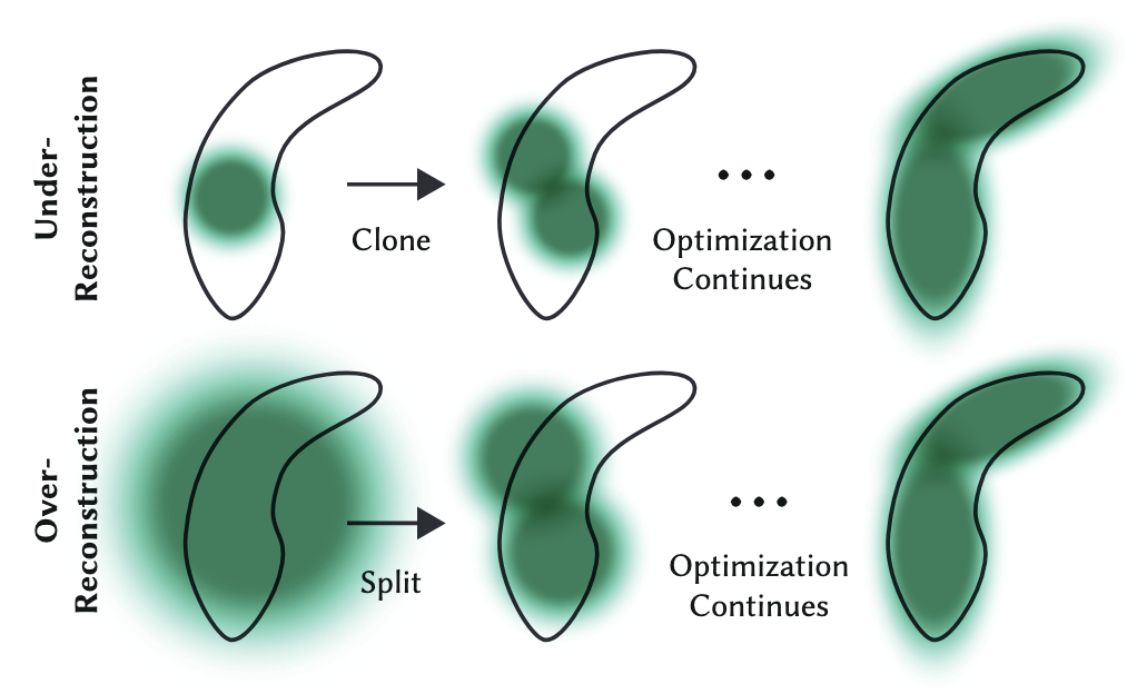
The optimization step needs to be able to create geometry and also destroy or move geometry when needed. The adaptive control enables a scheme to densify the Gaussians. After optimization warm-up, the densification is performed at every 100 iterations. In addition, any Gaussian that is essentially transparent, and therefore does not have a contribution in the representation, with \(\alpha < \epsilon_\alpha\) is removed.
Figure 1. demonstrates the densification procedure for the adaptive control of Gaussians.
Simply put, the densification procedure clones a new Gaussian when the small-scale geometry is not sufficiently covered. In the opposite case, when the small-scale geometry is represented by one large splat, the Gaussian is then split in two. Optimization continues with this new set of Gaussians.
3. Fast Differentiable Rasterizer for Gaussians
Tiling and camera view frustum. The method first splits the screen into \(16\times16\) tiles and then culls the 3D Gaussians against the camera view frustum and each tile. Only the Gaussians with 99% confidence intersecting the frustum are kept. In addition, the Gaussians at extreme positions like the ones with means close to the near plane and far outside the view frustum are rejected.
Sorting. All Gaussians are instantiated concerning the number of tiles they overlap. Each instance is assigned a key that combines view space depth and tile ID, and the keys are sorted via single-fast GPU Radix sort.
Rasterization. Finally, a list for each tile is produced using the first and last depth-sorted entry that splats to a given tile. Rasterization is performed in parallel with one thread block for each tile. For rasterization, we launch one thread block for each tile. Each thread first loads the Gaussians into shared memory and then, for a given pixel, accumulates color and \(\alpha\) values by traversing the lists front to back.
This procedure enables fast overall rendering and fast sorting to allow approximate \(\alpha\)-blending and to avoid hard limits on the number of splats that can receive gradients.
Our Results
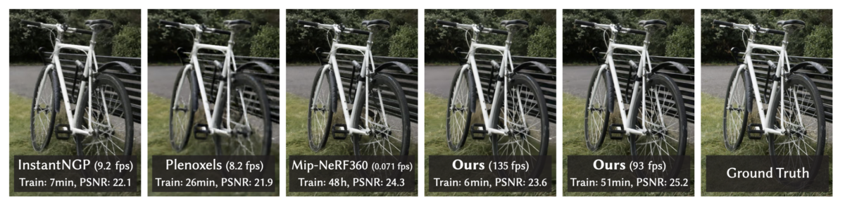
We test the 3D Gaussian splatting method, on the recently proposed dataset Neu3D [5]. Note that the original 3D Gaussian splatting work is limited to static scenes, while the Neu3D dataset provides dynamic scenes in time. Therefore, we provide the initial frames from each camera view of the flaming salmon scene as input. This corresponds to 19 frames of camera views, in total. We first execute the SfM method, in this case, COLMAP, on these frames to obtain the camera poses as discussed in Sec. 1. Next, we optimize the set of 3D Gaussians for a duration of 30K iterations.
Quantitative Evaluation: Metrics and Runtime
After 30K iterations of training, we report the metrics that are computed on the 3D Gaussian splatting method. \(L_1\) loss corresponds to the average difference between the set of training images and the rendered images as in Sec. 2.1 (Eq. 4). PSNR, or Peak Signal-to-Noise Ratio, corresponds to the ratio between the maximum possible power of a signal and the power of corrupting noise that affects the fidelity of its representation, measured in decibels. The memory row shows how much memory space the resulting representation occupies.
L1 loss [30K]
0.0074
PSNR [30K]
37.8426 dB
Memory [PLY]
162,5 MB
Table 1. shows the metrics for 3D Gaussian splatting on the flaming salmon scene of Neu3D.
We additionally report the runtime for the first two components, i.e. executing the SfM method to initialize the Gaussians and optimizing the Gaussians to obtain the resulting scene representation. The third component, rasterization, is performed in real time.
COLMAP – Elapsed time
0.013 minutes
Training Splats [30K]
10 minutes
Table 2. shows the runtime for 3D Gaussian splatting on the flaming salmon scene of Neu3D.
Qualitative Evaluation
We demonstrate the results from the model trained on the initial camera frames of the flaming salmon scene of Neu3D. We provide the real-time rendering results from the viewer where the camera is moving in space in Fig. 2.
Figure 2. shows the results of real-time rendering on SIBR viewer.
Conclusion and Future Work
3D Gaussian splatting is the first approach that truly allows real-time, high-quality radiance field rendering while requiring training times competitive with the fastest previous methods. One of the greatest limitations of this method comes from the memory consumption as the GPU memory usage can rise to ~20GB during training and therefore results in high storage costs. Second, the scenes that 3D Gaussian splatting is concerned with are static and do not incorporate an additional dimension to space, i.e. time. Recent work addresses these limitations through quantization and improvements on Gaussian representation to represent both time and space which we will discuss in the next post.
References
[1] Mildenhall, B., Srinivasan, P. P., Tancik, M., Barron, J. T., Ramamoorthi, R., & Ng, R. (2021). Nerf: Representing scenes as neural radiance fields for view synthesis. ECCV 2020.
[2] Kerbl, B., Kopanas, G., Leimkühler, T., & Drettakis, G. 3D Gaussian Splatting for Real-Time Radiance Field Rendering. ACM Trans. Graph. (SIGGRAPH) 2023.
[3] Snavely, N., M. Seitz, S., and Szeliski, R. Photo tourism: exploring photo collections in 3D. ACM Trans. Graph. (SIGGRAPH) 2006.
[4] Zwicker, M., Pfister, H., Van Baar, J., and Gross, M. EWA volume splatting. In Proceedings Visualization, VIS’01. IEEE, 2001.
[5] Li, T., Slavcheva, M., Zollhoefer, M., Green, S., Lassner, C., Kim, C., Schmidt, T., Lovegrove, S., Goesele, M., Newcombe, R., et al. Neural 3d video synthesis from multi-view video. CVPR 2022.