By: Judy Chiang, Natasha Diederen, Erick Jimenez Berumen
Project mentor: Christian Hafner
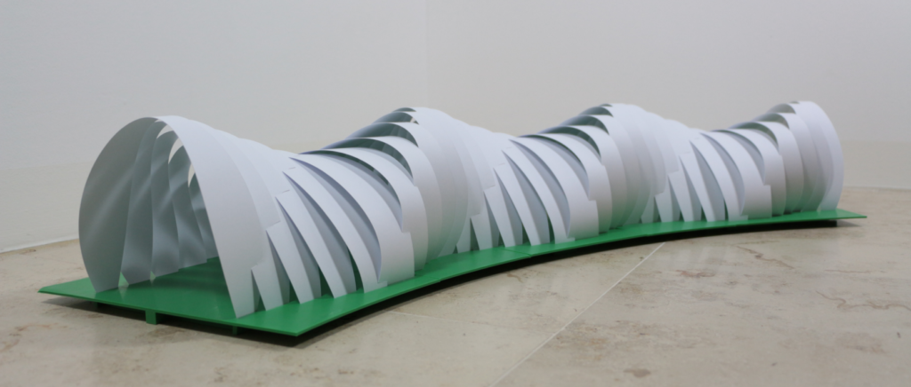
Architects often want to create visually striking structures that involve curved materials. The conventional way to do this is to pre-bend materials to form the shape of the desired curve. However, this generates large manufacturing and transportation costs. A proposed alternative to industrial bending is to elastically bend flat beams, where the desired curve is encoded into the stiffness profile of the beam. Wider sections of the beam will have a greater stiffness and bend less than narrower sections of the beam. Hence, it is possible to design an algorithm that enables a designer or architect to plan curved structures that can be assembled by bending flat beams. This is a topic currently being explored by Bernd Bickel and his student Christian Hafner (our project mentor).
For the flat beam to remain bent as the desired curve, we must ensure that the beam assumes this form at its equilibrium point. In Lagrangian mechanics, this occurs when energy is minimised, since this implies that there is no other configuration of the system which would result in lower overall energy and thus be optimal instead. Two different questions arise from this formulation. First, given the stiffness profile \(K\), what deformed shapes \(\gamma\) can be generated? Second, given a curve \(\gamma\), what stiffness profiles \(K\) can be generated? In answering the first problem we will find the curve that will result from bending a beam with a given width profile. However, we are more interested in finding the stiffness profile of a beam which will result in a curved shape \(\gamma\) of our choice. Hence, we wish to solve the second problem.
Below, we will give a full formulation of our main problem, and discuss how we transformed this into MATLAB code and created a user interface. We will conclude by discussing a more generalised case involving joint curves.
Problem formulation
To recap, the problem we want to solve is, given a curve \(\gamma \), what stiffness profiles \(K\) can be generated? For each point \(s\) on our curve \(\gamma: (0,\ell) \to \mathbb{R}^2\), we have values for the position \(\gamma(s)\), turning angle \(\alpha(s)\), and signed curvature \(\alpha'(s)\). In addition, we define the energy of the beam system to be \[W[\alpha] := \int_0^\ell K(s)\alpha'(s)^2 ds,\] where \(K(s)\) is the stiffness at point \(s\). At the equilibrium state of the system, \(W[\alpha]\) will take a minimum value. Intuitively, this implies that, in general, regions of larger curvature will have a lower stiffness. However, it is not true that two different points of equal curvature will have equal stiffness, since there are other factors at play.
Now, before finding the \(K\) that minimises \(W[\alpha]\), we must set additional constraints \[\alpha(0) = \alpha_0, \quad \alpha(\ell) = \alpha_\ell\] and \[\gamma(0) = \gamma_0, \quad \gamma(\ell) = \gamma_\ell.\] In words, we are fixing the turning angles (tangents) and positions of the two boundary points. These constraints are necessary, since they dictate the position in space where the curve begins and ends, as well as the initial and final directions the curve moves in.
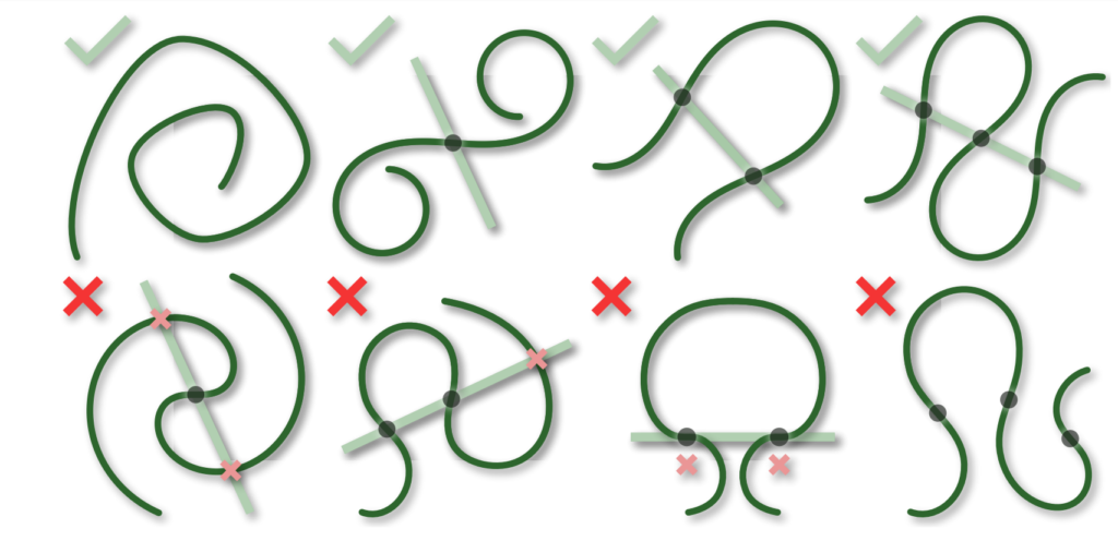
We have now formulated a problem that can be solved using variational calculus. Without going into detail, we find that stationary points of this function are given by the equation \[K \kappa = a + \langle b, \gamma \rangle,\] where \(\kappa\) is the signed curvature (previously \(\alpha’\)), and \(a \in \mathbb{R}\) and \(b \in \mathbb{R}^2\) are constants to be found. However, a stiffness profile cannot be generated for all curves \(\gamma\). More specifically, it was shown by Bernd Bickel and Christian Hafner that a solution exists if and only if there exists a line \(L\) that intersects \(\gamma\) exactly at its inflections. With this information in hand, we can begin to create a linear program that computes the stiffness function \(K\).
Creating a linear programme
In order to find the stiffness \(K\), we need to solve for the constants \(a\) and \(b\) in the equation \( K \kappa = a + \langle b, \gamma \rangle \), which can be discretised to \[ K(s_i) = \frac{a + \langle b, \gamma(s_i) \rangle }{\kappa(s_i)}.\] It is possible that there is more than one solution to \(K\), so we want some way to determine the “best” stiffness profile. If we think back to our original problem, we want to ensure that our beam is maximally uniform, since this is good for structural integrity. Hence, we solve for \(a\) and \(b\) in the above inequality in such a way that the ratio between maximum and minimum stiffness is minimised. To do this we set the minimum stiffness to an arbitrary value, for example 1, and then constrain \(K\) between 1 and \(M = \text{min}_i K_i\), thus obtaining the inequality \[1 \leq \frac{a + \langle b, \gamma(s_i) \rangle }{\kappa(s_i)} \leq M.\] This can be solved using MATLAB’s linprog function (read the documentation here). In this case, the variables we want to solve for are \(a \in \mathbb{R}\), \(b \in \mathbb{R}^2\), and \(M\) (a scalar we want to minimise). So, using the linprog documentation \(x\) is the vector \((a,b_1,b_2,M)\) and \(f\) is the vector \((0,0,0,1)\), since \(M\) is the only variable we want to minimise. Since linprog only deals with inequalities of the form \(A \cdot x \leq b\), we can split the above inequality into two and write it in terms of the elements of \(x\), like so: \[-\Bigg(\frac{1}{\kappa(s_i)}a + \frac{\gamma_x(s{i})}{\kappa(s_i)}b_1 + \frac{\gamma_y(s_{i})}{\kappa(s_i)}b_2 + 0\Bigg) \leq -1,\] \[\frac{1}{\kappa(s_i)}a + \frac{\gamma_x(s_{i})}{\kappa(s_i)}b_1 + \frac{\gamma_y(s_{i})}{\kappa(s_i)}b_2 -M \leq 0.\]
These two equations are of a form that can be easily written into linprog to obtain the values of \(a\), \(b\) and \(M\) and hence \(K\).
User Interface
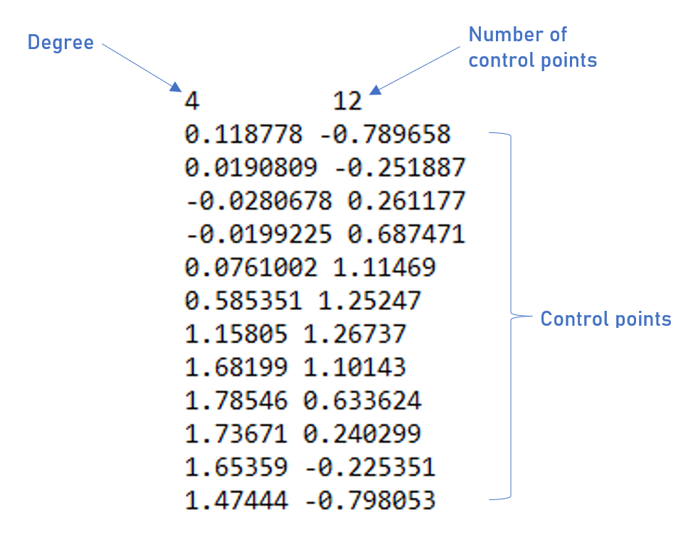
Once we solved the linear program outlined above, we created a user interface in MATLAB that would allow users to draw and edit a spline curve and see the corresponding elastic strip created in real time. Custom splines can be imported as a .txt file in the following format
or alternatively, the file that is already in the folder can be used. Users can then run the user interface and edit the spline in real time. To add points, simply shift-click, and a new point will be added at the midpoint between the selected point and the next point. The user can right-click to delete a point, and left-click and drag to move points around. If there are zero or one control points remaining, then the user can add a new point where their mouse cursor is by shift-clicking. The number of control points must be greater than or equal to the degree plus one for the spline to be formed.
There are certain cases in which the linear program cannot be solved. In these cases the elastic strip is not plotted, and the user must move the control points around until it is possible to create a strip.
Here is the link to the GitHub repository, for those who want to try the user interface out.
Joints Between Two or More Strips
The current version of our code is able to generate elastic strips for any (feasible) spline curve generated by the user. However, an as of yet unsolved problem is the feasibility condition for a pair of elastic strips with joints. Solving this problem would allow us compute a pair of stiffness functions \(K_1\) and \(K_2\) that yield elastic strips that can be connected via slots at the fixed joint locations. With a bit of maths we were able to derive the equilibrium equations that would produce such stiffness functions. Suppose the two spline curves are given by \(\gamma_{1}: [0,\ell_{1}] \to \mathbb{R}^2\) and \(\gamma_{2}: [0,\ell_{2}] \to \mathbb{R}^2\) and that they intersect at exactly one point such that \(\gamma_{1}(t_a) = \gamma_{2}(t_b)\). Then we must solve the following two equations: \[ K_{1}(t) \kappa_{1}(t) = \left \{ \begin{array}{ll} a_1 + \langle b_1, \gamma_{1}(t) \rangle + \langle c, \gamma_{1}(t) \rangle & 0 \leq t \leq t_a \\ a_1 + \langle b_1, \gamma_{1}(t) \rangle + \langle c, \gamma_{1}(t_a) \rangle & t_a < t \leq \ell_{1} \end{array}\right. \] \[ K_{2}(t) \kappa_{2}(t) = \left \{ \begin{array}{ll} a_2 + \langle b_2, \gamma_{2}(t) \rangle – \langle c, \gamma_{2}(t) \rangle & 0 \leq t \leq t_b \\ _2 + \langle b_2, \gamma_{2}(t) \rangle – \langle c, \gamma_{2}(t_b) \rangle & t_b < t \leq \ell_{2} \end{array}\right. \]
Similar to the one-spline case, these can be translated into a linear program problem which can be solved. Due to the time constraint of this project, we were not able to implement this into our code and build an associated user interface for creating multiple splines. Furthermore, above we have only discussed the situation with two curves and one joint. Adding more joints would increase the number of unknowns and add more sections to the above piece-wise-defined functions. Lastly, we are still lacking a geometric interpretation for the above equations. All of these issues regarding the extension to two or more spline curves would serve as great inspiration for further research!