Categories
SGI research projects

Robust computation of the Hausdorff distance between triangle meshes

Authors: Bryce Van Ross, Talant Talipov, Deniz Ozbay

The SGI project titled Robust computation of the Hausdorff distance between triangle meshes originally was planned for a 2 week duration, and due to common interest in continuing, was extended to 3 weeks. This research was led by mentor Dr. Leonardo Sacht of the Department of Mathematics of the Federal University of Santa Catarina (UFSC), Brazil. Accompanying support was TA Erik Amezquita, and the project team consisted of SGI fellows, math (under)graduate students, Deniz Ozbay, Talant Talipov, and Bryce Van Ross. Here is an introduction to the idea of our project. The following is a summary of our research and our experiences, regarding computation of the Hausdorff distance. 

Definitions

Given two triangle meshes A, B in , the following are defined:

1-sided Hausdorff distance h: 

$$h(A, B) = \max\{d(x, B) : x\in A\} = \max\{\min\{\|x-y\|: x\in A\}: y\in B\}$$

where d is the Euclidean distance and |x-y| is the Euclidean norm. Note that h, in general, is not symmetric. In this sense, h differs from our intuitive sense of distance, being bidirectional. So, h(B, A) can potentially be a smaller (or larger) distance in contrast to h(A, B). This motivates the need for an absolute Hausdorff distance.

2-sided Hausdorff distance H: 

$$H(A,B) = \max\{h(A, B), h(B, A)\}$$

By definition, H is symmetric. Again, by definition, H depends on h. Thus, to yield accurate distance values for H, we must be confident in our implementation and precision of computing h.

For more mathematical explanation of the Hausdorff distance, please refer to this Wikipedia documentation and this YouTube video.

Motivation

Objects are geometrically complex and so too can their measurements be. There are different ways to compare meshes to each other via a range of geometry processing techniques and geometric properties. Distance is often a common metric of mesh comparison, but the conventional notion of distance is at times limited in scope. See Figures 1 and 2 below.

Figure 1: This distance is limited to the red vertices, ignoring other points of the triangles.
Figure 2: This distance ignores the spatial positions of the triangles. So, the distance is skewed to the points of the triangles, and not the contribution of the space between the triangles.

Figures from the Hausdorff distance between convex polygons. 

Our research focuses on robustly (efficiently, for all possible cases) computing the Hausdorff distance h for pairs of triangular meshes of objects. The Hausdorff distance h is fundamentally a maximum distance among a set of desirable distances between 2 meshes. These desirable distances are minimum distances of all possible vectors resulting from points taken from the first mesh to the second mesh. 

Why is h significant? If h tends to 0, then this implies that our meshes, and the objects they represent, are very similar. Strong similarity indicates minimal change(s) from one mesh to the other, with possible dynamics being a slight deformation, rotation, translation, compression, stretch, etc. However, if h >> 0, then this implies that our meshes, and the objects they represent, are dissimilar. Weak similarity indicates significant change(s) from one mesh to the other, associated with the earlier dynamics. Intuitively, h depends on the strength of ideal correspondence from triangle to triangle, between the meshes. In summary, h serves as a means of calculating the similarity between triangle meshes by maximally separating the meshes according to the collection of all minimum pointwise-mesh distances. 

Applications

The Hausdorff distance can be used for a variety of geometry processing purposes. Primary domains include computer vision, computer graphics, digital fabrication, 3D-printing, and modeling, among others. 

Consider computer vision, an area vital to image processing, having a multitude of technological applications in our daily lives. It is often desirable to identify a best-candidate target relative to some initial mesh template. In reference to the set of points within the template, the Hausdorff distance can be computed for each potential target. The target with the minimum Hausdorff distance would qualify as being the best fit, ideally being a close approximation to the template object. The Hausdorff distance plays a similar role relative to other areas of computer science, engineering, animation, etc. See Figure 3 and 4, below, for a general representation of h.

Figure 3: Hausdorff distance h corresponds to the dotted lined distance of the left image. In the right image, h is found in the black shaded region of the green triangle via the Branch and Bound Method. This image is found in Figure 1 of the initial reading provided by Dr. Leonardo Sacht.
Figure 4: Hausdorff distance h corresponds to the solid lined distance of the left image. This distance is from the furthest “leftmost” point of the first mesh (armadillo) to the closest “leftmost” point of the second mesh. This image is found in Figure 5 of the initial reading provided by Dr. Leonardo Sacht.

Branch and Bound Method

Our goal was to implement the branch-and-bound method for calculating H. The main idea is to calculate the individual upper bounds of Hausdorff distance for each triangle meshes of mesh A and the common lower bound for the whole mesh A. If the upper bound of some triangle is greater than the general lower bound, then this face is discarded and the remaining ones are subdivided. So, we have these 3 main steps:

1. Calculating the lower bound

We define the lower bound as the minimum of the distances from all the vertices of mesh A to mesh B. Firstly, we choose the vertex P on mesh A. Secondly, we compute the distances from point P  to all the faces of mesh B. The actual distance from point P to mesh B is the minimum of the distances that were calculated the step before. For more theoretical details you should check this blog post: http://summergeometry.org/sgi2021/finding-the-lower-bounds-of-the-hausdorff-distance/

The implementation of this part:

Calculating the distance from the point P to each triangle mesh T of mesh B is a very complicated process. So, I would like not to show the code and only describe it. The main features that should be considered during this computation is the position of point P relatively to the triangle T. For example, if the projection of point P on the triangle’s plane lies inside the triangle, then the distance from point P to triangle is just the length of the corresponding normal vector. In the other cases it could be the distance to the closest edge or vertex of triangle T.

During testing this code our team faced the problem: the calculating point-triangle distance takes too much time. So, we created the bounding-sphere idea. Instead of computing the point-triangle distance we decided to compute point-sphere distance, which is very simple. But what sphere should we pick? The first idea that sprung to our minds was the sphere that is generated by a circumscribed circle of the triangle T. But the computation of its center is also complicated. That is why we chose the center of mass M as the center of the sphere and maximal distance from M to each vertex of triangle T. So, if the distance from the point P to this sphere is greater than the actual minimum, then the distance to the corresponding triangle is exactly not the minimum. This trick made our code work approximately 30% faster. This is the realization:

2. Calculating the upper bounds

Overall, the upper bound is derived by the distances between the vertices and  triangle inequality. For more theoretical details you should check this blog post: http://summergeometry.org/sgi2021/upper-bound-for-the-hausdorff-distance/

During testing the code from this page on big meshes our team faced the memory problem. On the grounds that we tried to store the lengths that we already computed, it took too much memory. That is why we decided just compute these length one more time, even though it takes a little bit more time (it is not crucial):

3. Discarding and subdividing

The faces are subdivided in the following way:  we add the midpoints and triangles that are generated by the previous vertices and these new points. In the end, we have 4 new faces instead of the old one. For more theoretical details you should check this blog post: http://summergeometry.org/sgi2021/branch-and-bound-method-for-calculating-hausdorff-distance/

Results

Below are our results for two simple meshes, first one being a sphere mesh and the second one being the simple mesh found in the blog post linked under the “Discarding and subdividing” section.
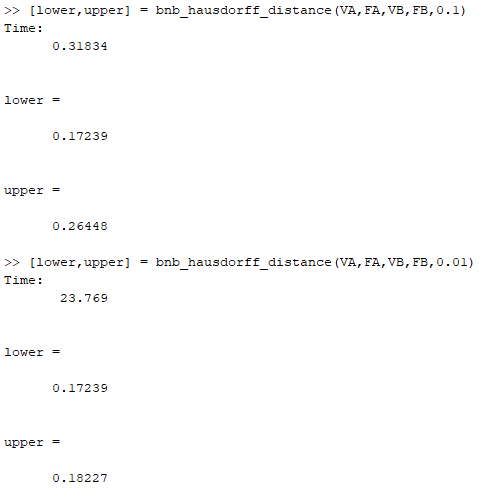
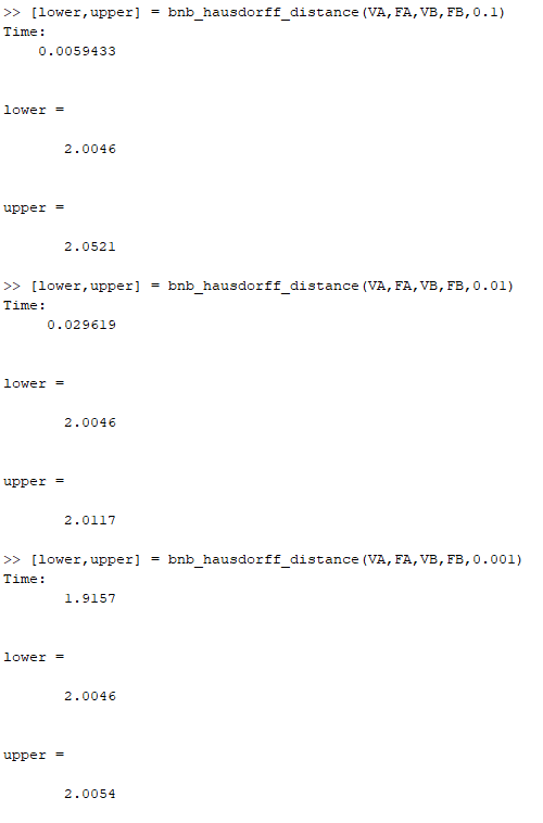
Figure 5: Results for a sphere mesh with different tolerance levels
Figure 6: Results for a smaller, simple mesh with different tolerance levels

Conclusion

The intuition behind how to determine the Hausdorff distance is relatively simple, however the implementation of computing this distance isn’t trivial. Among the 3 tasks of this Hausdorff distance algorithm (finding the lower bound, finding the upper bound, and finding a triangular subdivision routine), the latter two tasks were dependent on finding the lower bound. We at first thought that the subdivision routine would be the most complicated process, and the lower bound would be the easiest. We were very wrong: the lower bound was actually the most challenging aspect of our code. Finding vertex-vertex distances was the easiest aspect of this computation. Given that in MATLAB triangular meshes are represented as faces of vertex points, it is difficult to identify specific non-vertex points of some triangle. To account for this, we at first used computations dependent on finding a series of normals amongst points. This yielded a functional, albeit slow, algorithm. Upon comparison, the lower bounds computation was the cause of this latency and needed to be improved. At this point, it was a matter of finding a different implementation. It was fun brainstorming with each other about possible ways to do this. It was more fun to consider counterexamples to our initial ideas, and to proceed from there. At a certain point, we incorporated geometric ideas (using the centroid of triangles) and topological ideas (using the closed balls) to find a subset of relevant faces relative to some vertex of the first mesh, instead of having to consider all possible faces of the secondary mesh. Bryce’s part was having to mathematically prove his argument, for it to be correct, but only to find out later it would be not feasible to implement (oh well). Currently, we are trying to resolve bugs, but throughout the entire process we learned a lot, had fun working with each other, and gained a stronger understanding of techniques used within geometry processing.

In conclusion, it was really fascinating to see the connection between the theoretical ideas and the implementation of an algorithm, especially how a theoretically simple algorithm can be very difficult to implement. We were able to learn more about the topological and geometric ideas behind the problem as well as the coding part of the project. We look forward to finding more robust ways to code our algorithm, and learning more about the mathematics behind this seemingly simple measure of the geometric difference between two meshes.
Categories
SGI research projects

Branch-and-bound method for calculating Hausdorff distance

This week I worked on the “Robust computation of the Hausdorff distance between triangle meshes” project with our mentor Dr. Leonardo Sacht, TA Erik Amezquita and my team Talant Talipov and Bryce Van Ross.

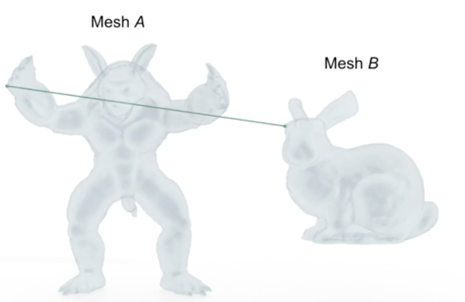
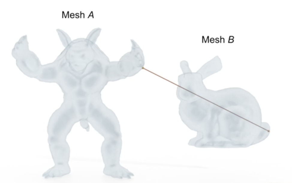
We started our project by doing some initial reading about the topic. Hausdorff distance from triangle meshes A to B is defined as $$h(A,B) = \max_{p \in A}d(p,B)$$ where d is the Euclidean norm. Finding the Hausdorff distance between two triangle meshes is one way of comparing these meshes. We note that the Hausdorff distance from A to B might be different from the Hausdorff distance from B to A, as you can see in the figure below, so it is important to distinguish which one is being computed.

Figure 1: Hausdorff distance from Mesh A to Mesh B
Figure 2: Hausdorff distance from Mesh B to Mesh A

Finally we define $$H(a,b) = \max{h(A,B), h(B,A)}$$ and use this value that is symmetric when comparing triangle meshes A and B.

Our first task was to implement Branch and Bound methods for calculating this distance. Suppose we want to calculate the Hausdorff distance from mesh A to mesh B. There were three main steps in the algorithm to do this: calculation of the upper and lower bound for the Hausdorff distance, and discarding and subdividing triangles according to the values of the upper and lower bound. 

The upper bound for each triangle in A is calculated by taking the maximum of the distances from the given triangle to every vertex in B.  The lower bound is calculated over A by taking the minimum of the distances from each vertex p in A to the triangle in B that is closest to p. If a triangle in A has an upper bound that is less than the lower bound, the triangle is discarded. After the discarding process, the remaining triangles are subdivided into four triangles and the process is repeated with recalculation of the upper bounds and the lower bound. The algorithm is run until the values for the upper and lower bound are within some ε of each other. Ultimately, we get a triangle region that contains the point that realizes the Hausdorff distance from A to B.

To implement this method, my teammates tackled the upper and lower bound codes while I wrote an algorithm for the discarding and subdividing process:

We ran this algorithm with testing values u = [1;2;3;4;5] and l = 3 and got these results:

Figure 3: Initial mesh
Figure 4: After discarding and subdividing

As expected, the two triangles that had the upper bound of 1 and 2 were discarded and the rest were subdivided.

 The lower bound algorithm turned out to be more challenging than we anticipated, and we worked together to come up with a robust method. Currently, we are working on finishing up this part of the code, so that we can run and test the whole algorithm. After this, we are looking forward to extending this project in different directions, whether it is a more theoretical analysis of the topic or working on improving our algorithm!

Categories
Talks

Week 5 Talks Summary

Authors: Bryce Van Ross, Deniz Ozbay, Talant Talipov

The following is a summary of three Week 5 talks, presented on behalf of students in the MIT Summer Geometry Institute. These summaries were made by members of the team of the Hausdorff Distance group. Topics include: Partitioned Solid-Fluid Coupling, Graduate School Panel and Q&A, and Developments in Smooth Optimization Contact.

Partitioned Solid-Fluid Coupling

This talk was presented by Dr. Tamar Shinar at University of California, Riverside. I liked this talk for several reasons. From an introductory physics background, we are aware that forces act on multiple objects. Depending on the type of object, certain forces behave differently with respect to the object and we use certain equations to model this interaction. However, as the system of objects becomes mixed, our use of forces becomes more complex. So, the modeling efforts must adapt accordingly. This lecture focused on how to model fluid-structure interaction (FSI), commonly referred to as solid-fluid coupling, via numerical algorithms, and discussed related applications. Examples of applications typically include fluid dynamics or animation. As suggested by Dr. Shinar, more intuitive, concrete examples are modeling the flight of a bird in the air (Figure 1), or the movement of a straight hair flip relative to a medium of water (Figure 2).

Figure 1: A bird (solid) flying in the air (fluid) adjacent to water droplets (another fluid). Image from unsplash.com/
Figure 2: A woman (solid) flipping her hair in a pool of water (fluid). Image from unsplash.com/

Solid-fluid coupling models the dynamics of fluids and solids. Specifically, these dynamics are computed simultaneously, which can be problematic. The challenge in this field is to make it less so, while ensuring a reflective representation of the physical forces at work. In 1- way coupling, the solid (or fluid) affects the fluid (solid), but not vice versa. This is not the case for 2-way coupling, where both objects affect each other, imposing more constraints upon the system. To account for each object’s phenomena, there exists solid and fluid handlers to model these phenomena, respectively. These solvers utilize a variety of boundary conditions, familiar to us from past math/physics courses, such as the Dirichlet, Navier-Stokes, and Neumann equations. Depending on the object and conditions, desirable properties are optimized. For solids, these would be mass and acceleration, whereas for fluids, these are position and velocity. The solution lies in the mixed-solver, and which numerical methods best model these behaviors.

There are multiple options to go about optimizing coupled-interaction. Partitioning the solver is a popular approach. In this approach, fixed point iteration and Newton’s method are strategies that solve the nonlinear system of equations, linearizing the 2-way coupling in terms of the solid and fluid. The partitioned methods tend to be more modular and easier to implement. In contrast, monolithic methods are more stable, have better performance, and handle closed regions better. In comparison to each other, their strengths are the other’s weaknesses. Common risks are that iterations can be computationally expensive and/or that they won’t converge at all. This is remedied by incorporating a reduced model interface (RMI), which serves as an intermediary lightweight solver between the solid and fluid. In effect, the RMI helps estimate tricky Jacobians in a least-weight sense. Dr. Shinar’s research specifically compares these numerical schemes in reference to an under-relaxation variable, which optimizes solution oscillations and aids in stability. The smaller this value, the slower and less efficient the computational time, in tradeoff for increased stability. The takeaways here are that the partition approach in isolation fails in terms of convergence, and the Partition-Coupling and RMI under low under-relaxation will yield optimal convergence in the shortest time. There still remain certain bounded regions, like (incompressible) Dirichlet regions, which interfere with the dynamics of known solid-fluid coupling techniques, but this has yet to be explored. For more information regarding Dr. Shinar’s research, please refer here.

An extended partitioned method for conservative solid-fluid coupling (Video from YouTube)

Developments in Smooth Optimization Contact

Professor Chenfanfu Jiang’s talk on “Developments in Smooth Optimization Contact” was really interesting for many reasons. Essentially the problem they were trying to solve was “How to model contact as a smooth problem”. This helps us accurately simulate solids which allows us to create realistic animations and benefits industry fields that use these simulations. For example in the fashion industry, these simulations provide feedback to the design of the garment.

Firstly, Dr. Jiang presented different ways to approach the problem and the advantages and shortcomings of these approaches. Then, he gave a formulation of how they came up with a solution using these, which was really interesting as it combined various approaches to come up with a better working algorithm. The research problem was also simple to understand but the tools used to solve the problem were very advanced, which was also very intriguing. 

To solve this problem three main tools were used: nonlinear optimization based integrator which simulated large deformation with large steps, variational frictional contact and its extension to higher dimensions. To start with, the solution is an optimization based time integrator for electrodynamics. It is based on incremented time steps, which creates an entirely new problem at each time step. The ODE consists of an inertia term and elasticity term – which makes the problem harder as the elasticity term can be highly nonlinear and non convex. This simulates deformations based on squashing and stretching. For a more physically accurate solution, contact is added as a constraint. This constraint in the form of an inequality, makes the differential equation even harder to solve. To overcome this challenge, different approaches were developed based on previous ways to solve the problem.

The difficulty arises from the fact that the formulated constraints and ODEs that are non-smooth and non-linear, for example, when the distance between objects is zero, we have a non-smooth constraint. To overcome this, the problem is turned into a smooth and unconstrained problem by using the incremental potential contact method which guarantees intersection and parameter tuning free simulations which are stable and accurate, and the barrier method, which turns the problem into an unconstrained problem where Newton iteration can be applied.

Dr. Jiang also discussed some methods that can improve their algorithm such as clamping the barrier function, and the shortcomings such as the difficulty of implementing friction in the optimization problem. Again, the challenges arise from the function becoming non-smooth, which he mentioned can be solved by approximately defining the variational friction as a smooth function.

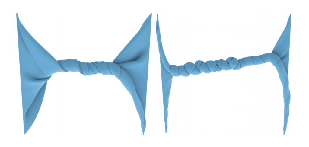
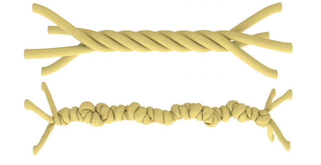
The most intriguing part of the talk was how they were able to build on existing approaches to turn the problem into a smooth one. Although the techniques they used were very advanced, the idea behind the solution was simple to understand. The simulations (especially the twisting of the cloth) Dr. Jiang showed were also really interesting; it was fascinating to see the difference between two simulations of the same object and how they become visibly more accurate as the constraints change.

Figure 3: Twisting of a cloth (image from https://ipc-sim.github.io/file/IPC-paper-350ppi.pdf)
Figure 4: Rod twist (image from https://ipc-sim.github.io/file/IPC-paper-350ppi.pdf)

Graduate School Panel

Last week I attended a talk about applications to PhD programs that was organized by Leticia Mattos Da Silva, Silvia Sellán, Jiayi Eris Zhang and Oded Stein.

One of the most exciting deals for every student is application for graduate programs. Most students are always confused with this procedure: they do not know what to write in a motivation letter and how to contact the prospective referee. All these questions were answered in this lecture. This lecture was filled with a lot of useful information about all the steps of applications to universities: from motivation letters to the choice of prospective scientific advisor. It was really interesting on the grounds that the lecturers experienced this procedure firsthand. Moreover, the speakers showed their own essays as successful examples.

As I know from this talk, the motivation letter has a specific structure. The applicant has to mention his previous research experience, why he wants to study exactly on this program, and why the university has to choose this person among the others. Furthermore, there should not be any information that is not relevant to the program: if you are applying to a PhD program in Mathematics, then you do not have to say about your background in knitting. The best moments were when the lecturer highlighted the most frequent mistakes of applicants and I realized that I did it in my motivation letter.

The recommendation letters are one of the most significant parts of the application. That is why the applicant should connect with his referee in advance. The best choice would be the person who did some research with you. In addition, you should have more referees in the case that the main ones reject.

It was a very valuable experience to listen to this lecture!