Fellows: Ikaro Penha Costa, Bereket Faltamo, Sahana Kargi, Van Le
Advisor: Oded Stein, University of Southern California
Volunteers: Lucas Valenca, Shaimaa Monem
MOTIVATION
The art of assembling model kits has always been a fascinating hobby; however, the process of generating these models is often limited to surfaces that can be easily flattened. Traditionally, it takes the 3D artists weeks or even months to create a model with detailed instructions on how to assemble it. Thus, this research aims to explore the potential of developing a tool that can automate the process of capturing the curvature of more complex objects, allowing the construction of any given surface. Our ambitions are to offer professionals an unprecedented level of creative freedom by opening up the possibilities of replicating more intricate shapes and from there, pave the way for novel applications in the engineering world.
METHODOLOGY
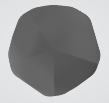
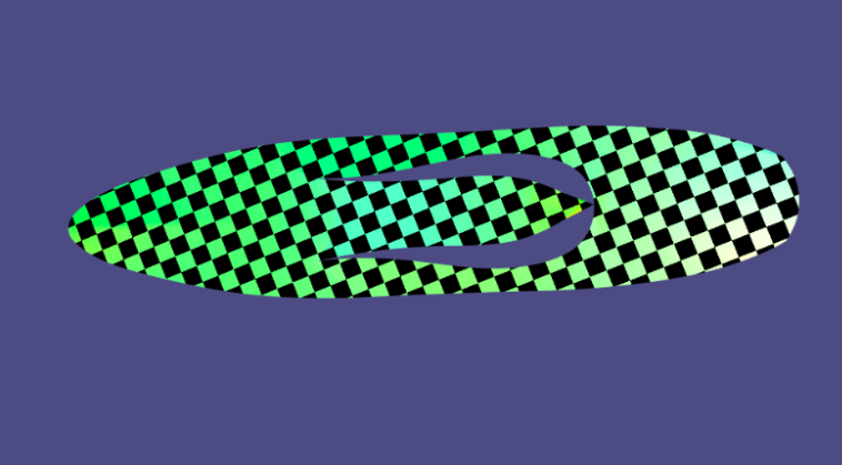
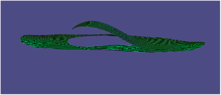
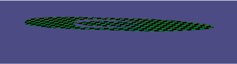
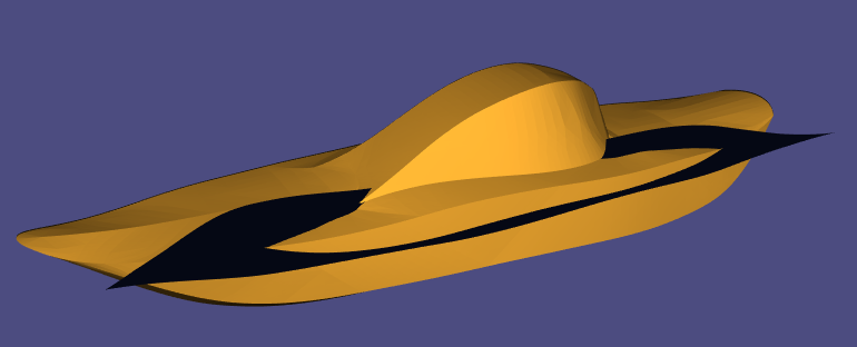
This project employs C++ and heavily uses the geometry processing library – libigl. For this research, the example objects are an icosahedron approximating the sphere and a mesh to a boat.
Segmentation into developable shapes
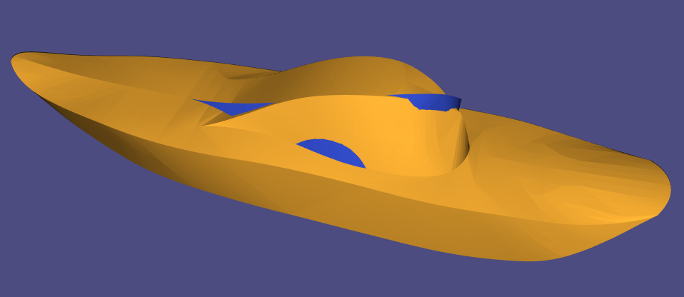
The first step is to determine whether it is a developable surface or not. In mathematics, a developable surface is a smooth surface with zero Gaussian curvature. We first took the boat and the icosahedral sphere and segmented them into parts that have zero Gaussian curvature. We checked the Gaussian curvature by using the Matlab code from Day 1 of the Tutorial Week. We could also do it with C++ by using this function.


Flattening pieces via corresponding homeomorphism
Once the shape is segmented, the next step is to flatten those segmented pieces. For this, we will use the geometry-processing-parameterization library and the Least Squares conformal mapping (LSCM) method. It works by finding and preserving the local angles and lengths between pieces. It aligns the centroids within the segments and then finds the optimal rotation, scaling, and translation using a least squares approach. Here are the results of implementing it on different segments of the boat.
Before LSCM After LSCM

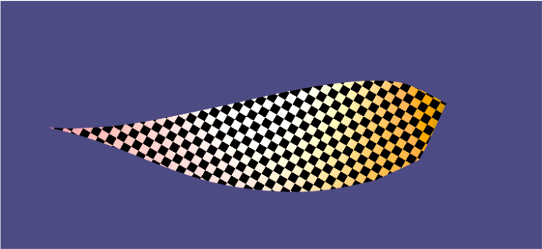
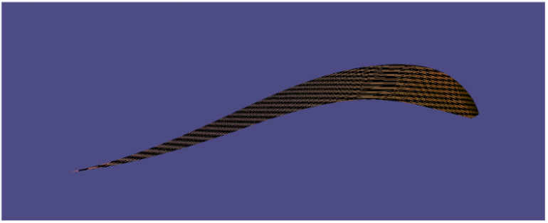
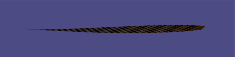

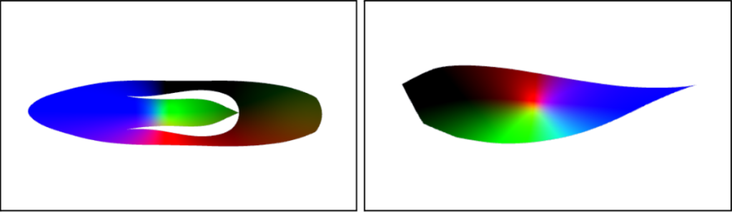
In addition to flattening the pieces, we also colored them according to their coordinates. We normalized the X, Y, and Z coordinates of all the vertices and colored them the coordinating RGB color. The goal is to use this colormap during reassembly so that the flattened pieces can be curved to the proper amounts.
Reassembling Pieces
In possession of the set of folded pieces, it naturally follows that each piece could be reconnected to revert this collection to the original object shape. This step is denominated reassembling instructions and essentially requires techniques of Shape Correspondence. That is, find a correspondence between a folded piece and the original shape.
Two main mathematical measures are involved in comparing the similarity of topological spaces: Hausdorff and Frechét distances. A more common implementation of bounds for Hausdorff distance is based on an energy optimization as discussed by Alec Jacobson in these tutorial notes. In this case, the Hausdorff distance is used to iteratively find the closest correspondence between a point in the source mesh and the entirety of the target mesh. This algorithm is Iterative Closest Point (ICP) and it is also available in libigl.


As seen in the image above, a segmented piece matches the correct place on the icosahedron after running the ICP algorithm. The ICP technique is, in summary, a sampling step of the mesh (VX, FX) and an optimization step in which each point in VX the objective function is to minimize the Hausdorff distance between this point and the target mesh (VY, FY). The libigl provides the point-to-normal implementation discussed in Jacobson’s notes, which is a form of Gauss-Newton optimization algorithm. This method requires an integer for the number of sample points in (VX, FX) and also an integer for the maximum number of iterations to be used in the minimization algorithm.
The number of sample points and maximum iterations is decisive in order to obtain reliable reassembling results. As a common fact in optimization, depending on the number of iterations and size of the model, the algorithm might be susceptible to being stuck at a local minimum. This is also the case with ICP, causing artifacts as the image below:
A valid approach to avoid this sinister reassembling is to generate different initial conditions so that the optimization algorithm might converge to different local minima. In this case, using the Eigen library, a set of uniformly random rigid transformations are applied to the piece before passing it to the ICP method. Since the Hausdorff distance is the objective function, the rigid transformation which causes ICP to produce the lowest Hausdorff distance is stored and then used to produce the final result.
However, research (and also life) is never linear. The approach described before would cause a few failed assertions throughout the label library. The assertions would be informed that the transformed mesh would have zero area. As the libigl area computation is robust, further investigations are necessary.
The investigations have determined the existence of overflow in the translation vector inside the ICP method. For the boat example, the entries in VX are originally in the magnitude of 101, and after some iterations of the ICP, the translation vector is applied to VX whose every entry would be numerically the same number in the magnitude of 1028; then, causing the transformed mesh to have zero area. In this case, the proposed remediation is to ignore the transformed initial pieces which would cause large entry-wise points in VX.
Hence, after performing each ICP iteration with the extra care of managing the translation vector entries, promising results were found as shown in the image below. Observe that the piece matches a similar side of the boat but not the correct side, it is placed in the mirrored side. In this case, a possibility is that it might be necessary to add more constraints to the initial conditions.
As finding the cause of zero areas has demanded significant time, the approach of adding more constraints to the initial conditions can be left as future work. For this, one can store information on the piece boundary in the segmentation step. This information could be used to point the ICP rotation and translation in the direction of the correct final place in the target shape at each iteration step. That is, try to point ICP rigid transformation to the original place of segmentation of each piece. Hopefully, this would cause correctness of results and faster convergence.
Reassembling Instructions with Edge Coloring
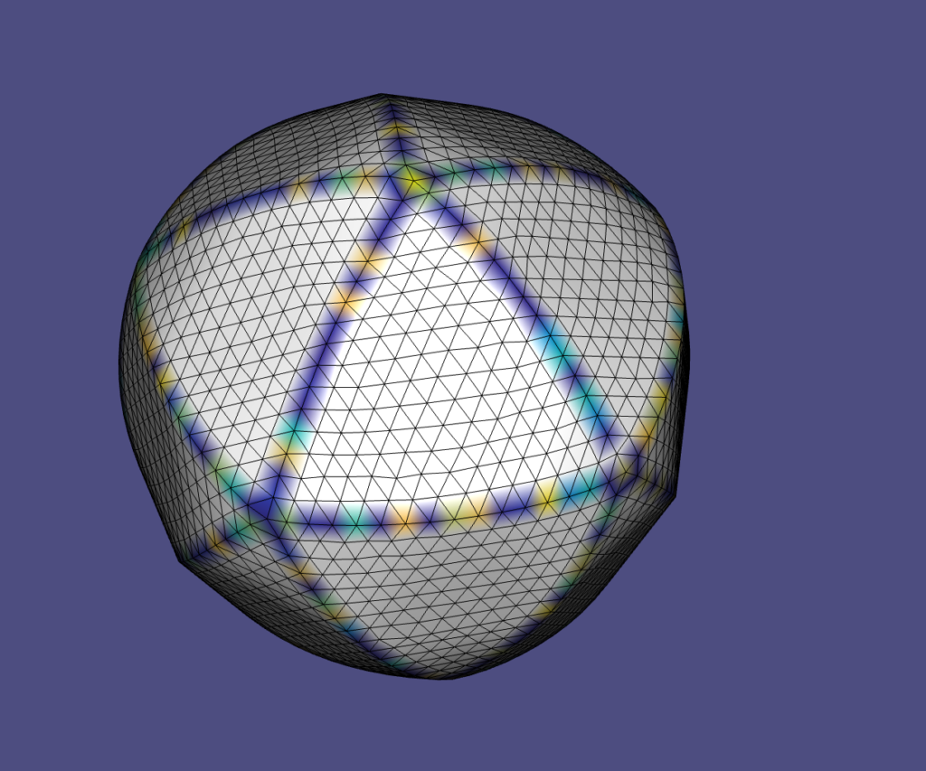
When putting the pieces back together we need a way to know which parts come together. In particular, we need to know which pieces have shared edges. That is where edge coloring helps. We color-coded each cutting line with random patterns so that the pieces will take part of the pattern with them. The color coding of the icosahedron can be seen below.
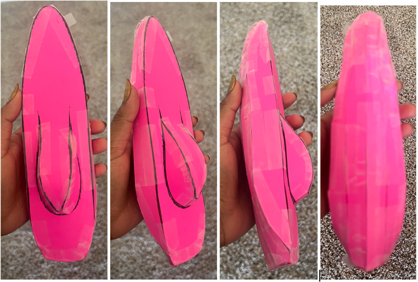
Real Life Assembly by Adding Tabs and Holes
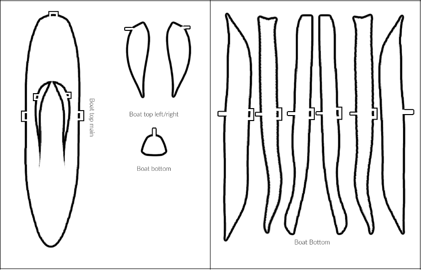
As a final step, we wanted to see how accurate our algorithm was in real life. We formatted and printed the images and assembled them. Some work is needed in ensuring that all the individual shapes are the proper size. Additionally, we added the tabs and holes to the segments so the pieces fit together.
Link to Repo
ACKNOWLEDGEMENTS
We would like to express our sincere gratitude to Professor Oded Stein for his instruction, guidance, and encouragement throughout this research.
We would also like to acknowledge the advice and recommendations of the volunteers – Lucas and Shaimaa for offering help, unique insights, and perspectives.
This research heavily used C++ and the library libigl.