Categories
Research

Building correspondences in multiresolution representations

By SGI Fellows:  Anna Cole, Francisco Unai Caja López, Matheus da Silva Araujo, Hossam Mohamed Saeed

I. Introduction

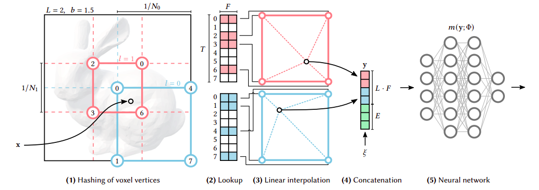
In this project, mentored by Professor Paul Kry, we are exploring properties and applications of multiresolution surface representations: surface meshes with different complexities and details that represent the same underlying surface.

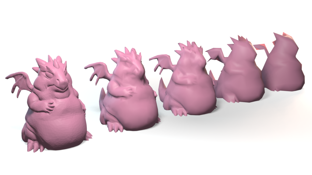
Frequently, the digital representation of intricate and detailed surfaces requires huge triangle meshes. For instance, the digital scan of Michelangelo’s statue of David [9] contains over 1 billion polygon faces and requires 32 GB of memory. The high level of complexity makes it costly to store and render the surface. Furthermore, applying standard geometry processing algorithms on such complex meshes requires huge computational resources. An alternative consists in representing the underlying surface using hierarchy of meshes, also known as multiresolution representations [2]. Each successive level of the hierarchy uses a mesh with lower geometric complexity while representing the same smooth surface. A hierarchy of meshes allows to represent surfaces at different resolutions, which is critical to handle complex geometric models. This form of representation provides efficiency and scalability for rendering and processing of complex surfaces, because the level of detail of the surface can be adjusted based on the hardware available. Figure 1 shows one example of a hierarchy of meshes. In this project we explore the construction of hierarchical representations of surface meshes combined with correspondences between different levels of the hierarchy.

Figure 1: a hierarchy of meshes built using mesh simplification.

One critical point of this construction is a mapping between meshes at different levels. Liu et al. 2020 [7] proposes a bijective map, named successive self-parameterization, that allows to correspond coarse and fine meshes on the multiresolution hierarchy. To build this mapping, successive self-parameterization requires a (i) mesh simplification algorithm to build the hierarchy of meshes and (ii) a conformal parameterization to map meshes on successive refinement levels to a common space. Our goal for this project is to investigate different applications of this mapping. In the next sections, we detail the algorithms to construct the hierarchy and the successive self-parameterization.

II. Mesh simplification

II.1. Mesh simplification using quadric error

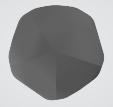
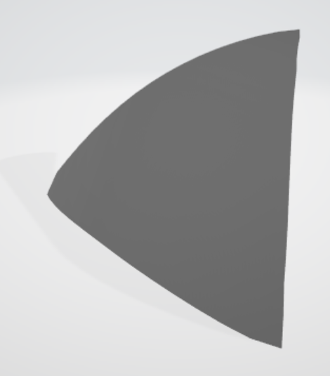
The mesh simplification algorithm studied was introduced in Garland and Heckbert 1997 [6] and is quite straightforward: it consists in collapsing various edges of the mesh sequentially. Specifically, in each iteration, two neighboring vertices \(v_i\) and \(v_j\) will be chosen and replaced by a single vertex \(\overline{v}\). The new vertex \(\overline{v}\) will inherit all neighbors of \(v_i\) and \(v_j\). In Animation 1 it is possible to see the possible result of two edge collapses in a triangle mesh.

Animation 1: consecutive edge collapses in a triangle mesh.

Suppose we have decided to collapse edge \((v_i,v_j)\). Then, \(\overline{v}\) is found as the solution of a minimization problem. For each vertex \(v_i\) we define a matrix \(Q_i\) so that \(v^TQ_iv\), with \(v=[v_x, v_y, v_z, 1]\), gives a measure of how far \(v\) is from \(v_i\). We choose \(\overline{v}\) minimizing \(v^T(Q_i+Q_j)v\). As for the choice of the \(Q\) matrices, we consider:

  • To each vertex \(v_i\) we associate the set of planes corresponding to faces that contain \(v_i\) and denote it \(\mathcal{P}(v_i)\).
  • For each face of the mesh we consider \(p=[a,b,c,d]^T\) such that \(v^Tp=0\) is the equation of the plane and \(a^2+b^2+c^2=1\). This allows us to compute the distance from a point \(v=[v_x,v_y,v_z,1]\) to the plane as \(\vert v^Tp \vert\).

Then, the sum of the squared distances from \(v\) to each plane in \(\mathcal{P}(v_i)\) would be

\(\displaystyle \sum_{p\in\mathcal{P}(v_{i})}(v^{T}p)^{2}= \sum_{p\in\mathcal{P}(v_{i})}v^{T}pp^{T}v = v^{T}\Bigg(\underbrace{\sum_{p\in\mathcal{P}(v_{i})}pp^{T}}_{{\text{choice of} }Q_{i}}\Bigg)v\)

Finally, we decide which edge to collapse by choosing \((v_i,v_j)\) minimizing the error \(\overline{v}^T(Q_i+Q_j)\overline{v}\). For the following iterations, \(\overline{v}\) is assigned the matrix \(Q_i+Q_j\). Animations 2 and 3 illustrates the process of mesh simplification using quadric error.

Animation 2: mesh simplification of Spot.
Animation 3: mesh simplification of Fennec Fox.

The algorithm can also run on meshes with boundaries. In Animation 4 we chose not to collapse boundary edges, which allows the boundaries to be preserved.

Animation 4: simplification of a mesh with boundaries. In this case, the boundary of the mesh is preserved.
II.2. Manifoldness and edge collapse validation

There are a variety of issues that can occur if we collapse each edge only based on the error quadrics \(Q_i+Q_j\). This is because the error quadric is only concerned with the geometry of the meshes but not the topology. So we needed to implement some connectivity checks to make sure the edge collapse wouldn’t result in a non-manifold case or change the topology of the mesh.

This can be visualized in Animation 5, where collapsing an interior edge consisting of two boundary vertices can create a non-manifold edge (or vertex). Another problematic case is collapsing an edge with its two vertices sharing more than two neighboring vertices, which would break manifoldness. We followed the criteria described in Liu et al. 2020 [7] and Hoppe el al. 1993 [5] to guarantee an manifold input mesh stays manifold after each collapse. Also, we added the condition where we compute the Euler characteristic \(\chi(M)\) before and after the collapse and if there is a change, we revert back and choose a different edge. In case all remaining edges are not valid for the collapse operation, we simply stop the collapsing process and move on to the next step.

Animation 5: examples of valid edge collapses (left and center figures, in blue) and an example of an edge collapse that generates non-manifold elements (right figure, in orange).

III. Mesh parameterization

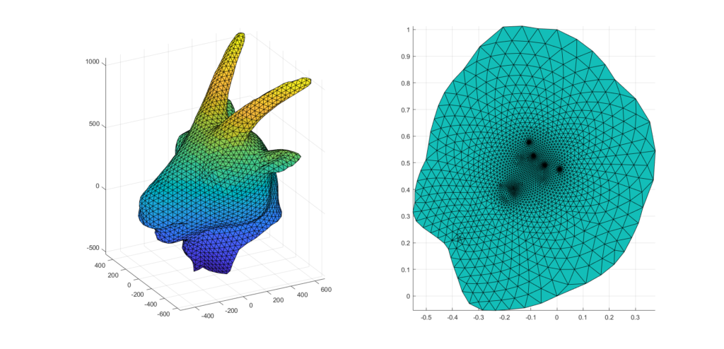
Mesh parameterization deals with the problem of mapping a surface to the plane. In our case, the surface is represented by a triangle mesh. This means that for every vertex of the triangle mesh we find corresponding coordinates on the 2D plane. More precisely, given a triangle mesh \(\mathcal{M}\), with a set of vertices \(\mathcal{V}\) and a set of triangles \(\mathcal{T}\), the mesh parameterization problem is concerned with finding a map \(f: \mathcal{V} \rightarrow \Omega \subset \mathbb{R}^{2}\). The effect of this mapping can be seen in Animation 6, where one 3D mesh is flattened to the 2D plane.

Animation 6: a triangle mesh embedded in \(\mathbb{R}^{3}\) is flattened to the 2D plane using a mesh parameterization algorithm.

This mapping enables all sorts of interesting applications. The most famous one is texture mapping: how to specify texture coordinates for each vertex of a triangle mesh such that you can map a region of an image to the mesh? Other applications include conversion of triangle meshes into parametric surfaces [11] e.g., T-Splines or NURBS and computational fabrication [12]. In this section we won’t give all the details about this field, but rather will focus on the aspects relevant to build mappings between meshes of different refinement levels on the hierarchical surface representation. We refer the interested reader to Hormann et al. 2007 [10] for an extensive treatment.

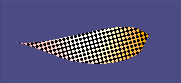
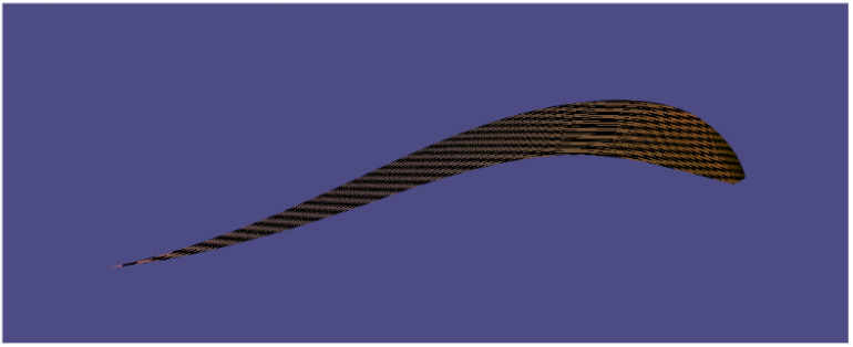
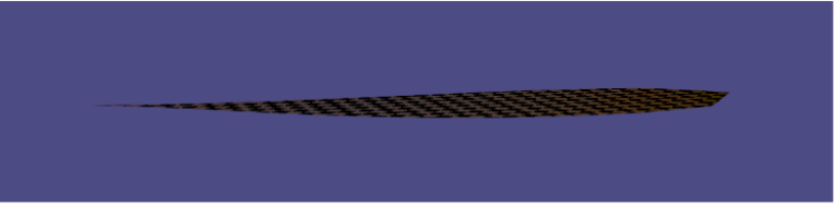
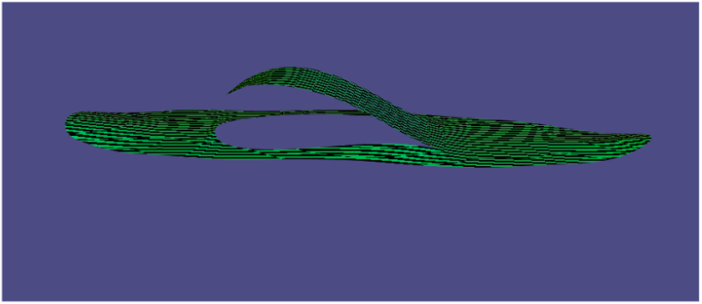
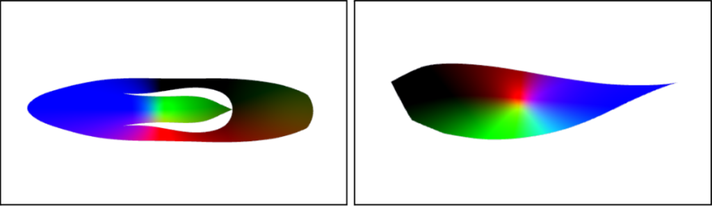
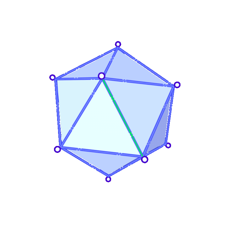
There are many different possibilities to define the mapping from the surface to the plane. However, this mapping usually introduces undesirable distortions. Depending on the construction used, the map may preserve areas, but not angles or orientations; conversely, it may preserve angles but not areas and lengths. This can be seen in Figure 2, where we can visualize angles and area distortions in the parameterized mesh.

Figure 2 : given a triangle mesh (left), we can map it to the 2D plane (center and right). This mapping can introduce angle distortions (center) and area distortions (right).

To create maps between meshes of different levels, Liu et al. 2020 [7] uses conformal mappings, which are maps that preserve angles. Conformal mappings are efficient to compute and provide theoretical guarantees, making it a common choice for many geometry processing tasks.

A conformal map is characterized by the Cauchy-Riemann equations:

\(\displaystyle \begin{align*} \frac{\partial v(x,y)}{\partial x} &= -\frac{\partial u(x,y)}{\partial y} \\ \frac{\partial v(x,y)}{\partial y} &= \frac{\partial u(x,y)}{\partial x} \end{align*}\)

or, more compactly,

\(\nabla u = \nabla v^{\bot}\)

Conformal mappings also have a strong connection with complex analysis, which leads to an alternative but equivalent formulation of the problem.

For arbitrary triangle meshes it is impossible to find an exact conformal mapping; only developable meshes (i.e., meshes with zero Gaussian curvature at every point) can be conformally parameterized. In most cases, this restriction is too severe. To work around this, it is possible to build a conformal mapping satisfying the previous equations as close as possible. In other words, we can associate it with an energy function to find the mapping that better approximates a conformal mapping using a least squares formulation:

\(E_{LSCM} = \int_{\mathbf{S}} \lVert \nabla u – \nabla v^{\bot} \rVert^2 dA\)

where \(S\) is the smooth surface represented by a triangle mesh \(\mathcal{M}\).

On a triangle mesh, the functions \(u(x, y), v(x,y)\) can be written with respect to the local orthonormal coordinate system of the triangle. Since the triangle mesh is a piecewise linear surface, the gradient of a function defined over the mesh is constant with respect to each triangle. This makes it possible to find the mapping that better approximates the Cauchy-Riemann equations for each triangle of the mesh. Hence, in this discrete setting, the previous equation can be rewritten as follows

\(\displaystyle \begin{align*} E_{LSCM} &= \sum_{t \in \mathcal{T}} A_{t} \left \lVert M_{t} \cdot \mathbf{v}_{t} – \begin{bmatrix}0 & -1 \\ 1 & 0 \end{bmatrix} M_{t} \cdot \mathbf{u}_{t} \right \rVert ^{2} \\ M_{t} &= \frac{1}{2 \cdot A_{t}} \cdot \begin{bmatrix} y_{j} – y_{k} & y_{k} – y_{i} & y_{i} – y_{j}\\ x_{k} – x_{j} & x_{i} – x_{k} & x_{j} – x_{i} \end{bmatrix} \end{align*}\)

where \(A_{t}\) denotes the area of each triangle with vertices represented by \((i, j, k)\). The solution of the discrete conformal energy described above are the coordinates \((u, v)\) in the 2D plane for each vertex of each triangle \(t\) in the set of triangles \(\mathcal{T}\) of the mesh \(\mathcal{M}\). More details can be found in Lévy et al. 2002 [4] and Desbrun et al. 2002 [13].

However, the trivial solution for this equation would be to set all coordinates \((u, v)\) to the same point and the energy would be minimized, which is not what we want. Therefore, to prevent this case, it is necessary to fix or pin two arbitrary vertices to arbitrary positions in the plane. This restriction generates a least squares problem with a unique solution. The choice of the vertices to be fixed is arbitrary but can have impact on the quality and numerical stability of the parameterization. For instance, there can be arbitrary area distortions depending on the vertices that are fixed. To prevent the problem of the trivial solution while preserving numerical stability, an alternative strategy is proposed by Mullen et al. 2008 [3] in which the system is reformulated to an equivalent eigendecomposition problem which avoid the need to pin any vertex.

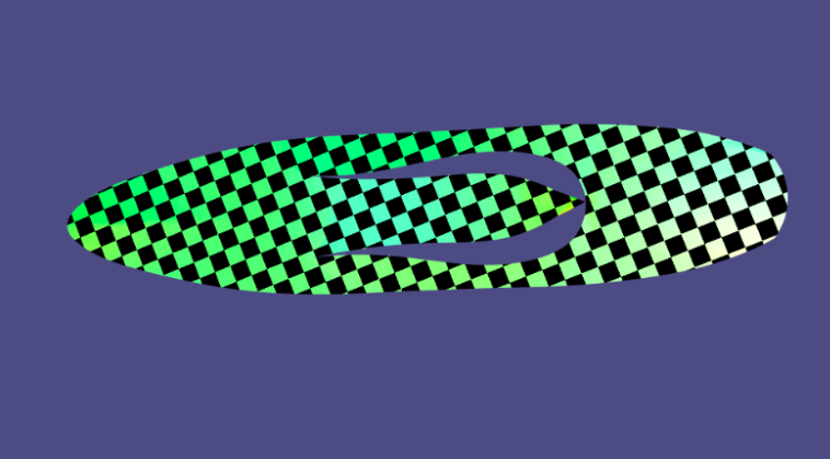
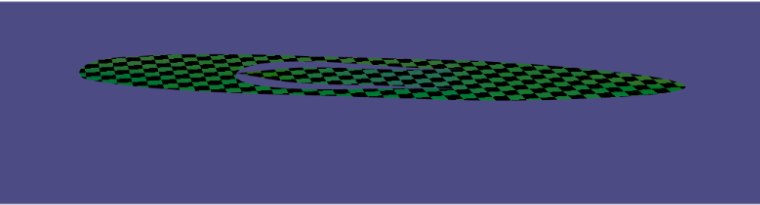
Figure 3 illustrates the least squares conformal mapping obtained for a triangle mesh with boundaries. Notice that the map obtained doesn’t necessarily preserve areas and lengths. Furthermore, as can be seen in the right plot of the figure, lots of details are grouped around tiny regions in the interior of the parameterized mesh.

Figure 3: a triangle mesh (left) and the resulting parameterized mesh in the plane (right).

This algorithm is a central piece to create a bijective map between meshes on different levels of the hierarchy.

IV. Successive self-parameterization

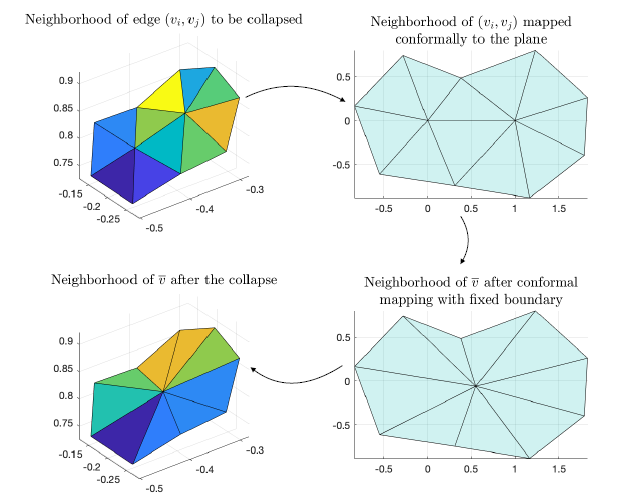
For each edge collapse, we use this procedure to create a bijective mapping between the original mesh, called \(\mathcal{M}^L\), and the mesh after an edge collapse, \(\mathcal{M}^{L-1}\). To construct a mapping from our coarsest mesh to finest mesh, we used spectral conformal parameterization as described in Mullen et al. 2008 [3] and build a successive mapping following the same procedure as Liu et al. 2020 [7]. As mentioned in the previous section, conformal mapping is a parameterization method that preserves angles. For a single edge collapse, \(\mathcal{M}^L\) and \(\mathcal{M}^{L-1}\) are the same except for the neighborhood of the collapsed edge. Therefore, if \((v_i,v_j)\) is the edge to be collapsed, we only need to build a mapping from the neighborhood of \((v_i,v_j)\) in \(\mathcal{M}^L\) to the neighborhood of \(\overline{v}\) in \(\mathcal{M}^{L-1}\). We do this in three steps:

  1. We first map the neighborhood of \((v_i,v_j)\) to the plane via conformal mapping.
  2. A key observation here is that the neighborhood of \(\overline{v}\in\mathcal{M}^{L-1}\) has the same boundary as the neighborhood of \((v_i,v_j)\) before the collapse. We then do a conformal mapping of the neighborhood of \(\overline{v}\in\mathcal{M}^{L-1}\) fixing the boundary so that the resulting 2D region is the same as before.
  3. Now we map points between the 3D neighborhoods using the shared 2D domain.

This process is illustrated in Figure 4.

Figure 4: a triangle mesh before and after the collapse (left column) and their corresponding parameterizations (right column). By mapping the mesh before and after the collapse to the plane, it is possible to create a bijective mapping between the two meshes.

We repeat this process successively for a certain number of collapses to arrive at the desired, coarsest mesh. We refer to the combination of these methods as successive self-parameterization, as described in Liu et al. 2020 [7]. In the implementation of our algorithm, we ran into problems with overlapping faces and badly shaped, skinny triangles. We discuss the mitigation of these problems in the next section.

V. Testing And Improvements

In each part of the project, we always tried to test and potentially improve its results. These helped improve the final output as discussed in Section VI – Results.

V.1. Quality checks for avoiding skinny triangles

To help solve the problem of skinny triangles, we implemented a quality check on the triangles of our mesh post-collapse using the following formula:

\(Q_{ijk}=\frac{4\sqrt{3}A_{ijk}}{l_{ij}^2+l_{jk}^2+l_{ki}^2}\)

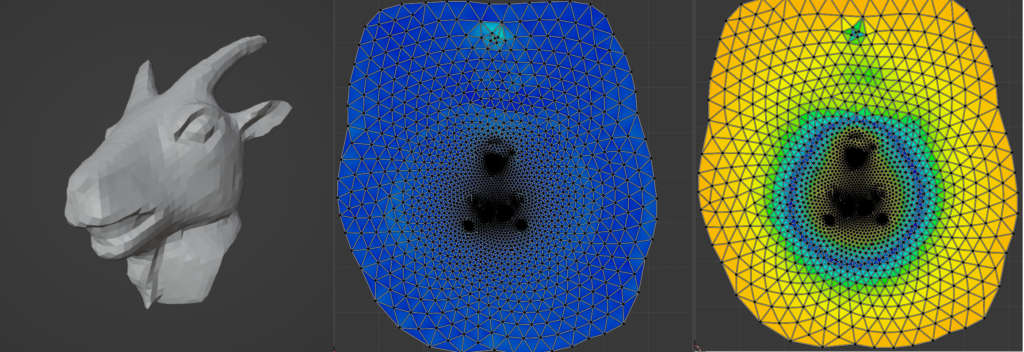
Here \(A\) is the area of a triangle, \(l\) are the lengths of the triangle edges, and \(i,j,k\) represent the indices of the vertices on the triangle. Values of \(Q\) closer to 1 indicate a high quality triangle, while values nearing 0 indicate a degenerate, poor quality triangle. We implemented a test that undoes a collapse if any of the triangles generated have a low value of \(Q_{ijk}\). Figure 5 shows an image with faces of varying quality. Red indicates low quality while green indicates high quality.

Figure 5: visualization of the quality of each triangle in a triangle mesh. A red triangle represents bad quality while a green triangle represents good quality.
V.2. The Delaunay Condition and Edge flips for avoiding skinny triangles

After testing the pipeline on multiple meshes and with different parameters, we realized that there was one issue. While the up-sampled mesh had good geometric quality (due to successive self-parameterization), the triangle quality was not very good. This is because the edge collapses can generally produce some skinny triangles.

To solve this, we implemented a local edge flip after each edge collapse. In that case, we check for edges that don’t satisfy the Delaunay Condition. The Delaunay condition is a good way to improve the triangle angles by penalizing obtuse angles.

Figure 6: example of a mesh that does not satisfy the Delaunay condition (left) and of a mesh that does satisfy the Delaunay condition (right).

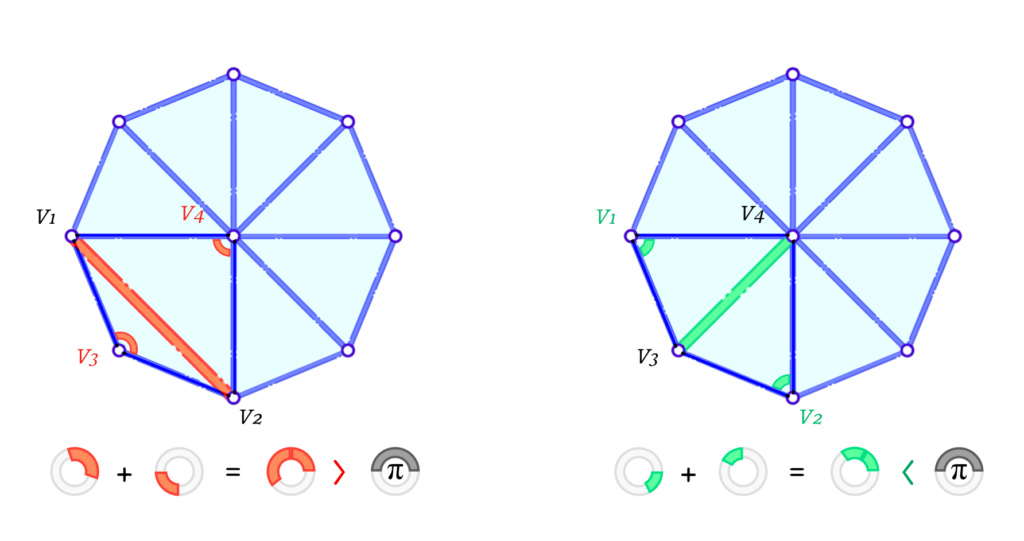
Figure 6 illustrates two cases where the left one violates the Delaunay condition while the one on the right satisfies it. Formally, for a given interior edge \(e_{1-2}\) connecting the vertices \(v_1\) and \(v_2\), and having \(v_3\) and \(v_4\) opposite to it on each of its 2 faces, it satisfies the condition if and only if the sum of the 2 opposite interior angles is less than or equal to \(\pi\). In other words:

\(\angle v_1 v_4 v_2 + \angle v_2 v_3 v_4 \leq \pi\)

As this makes it very unlikely to have obtuse angles, it eliminates some cases of skinny triangles. It is important to note that a skinny triangle can be produced even if all angles are acute, as one of them can be a very small angle. This is another case of skinny triangles but we have other checks mentioned before to help avoid such cases.

Figure 7: given an initial mesh (left), the edge collapse may generate skinny triangles (center). The edges of the triangles that violate the Delaunay condition are flipped (right).

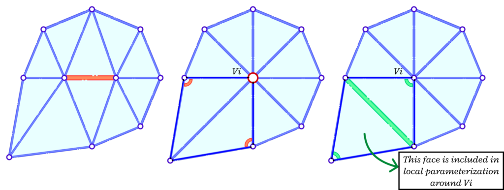
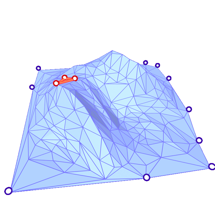
The edge flips are implemented right before the self-parameterization part. This is to improve triangle quality after each collapse. The candidate edges for a flip are only the ones that are connected to the vertex resulting from the collapse. We also need a copy of the face list before the flip to ensure the neighbourhood is consistent before and after the collapse when we go into the self-parameterization stage. Figure 7 shows an example of a consistent neighbourhood before the collapse, after the edge collapse and after the edge flip (in that order). We need to consider the face that is not any more a neighbor to the vertex to have a consistent mapping.

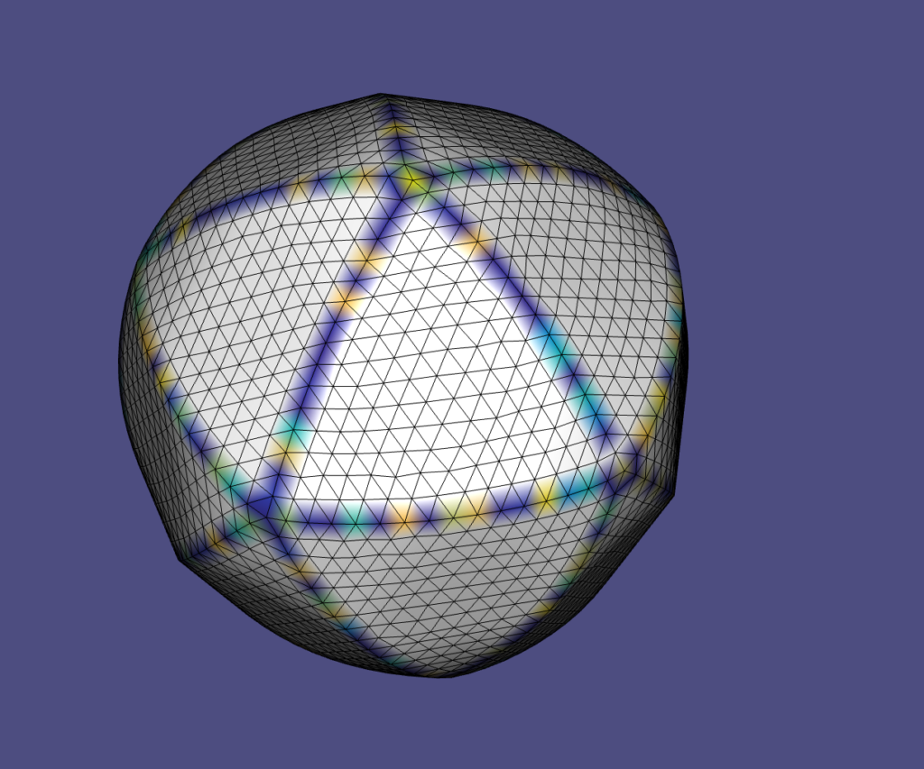
The addition of edge flips improved the triangle quality of the final mesh (after re-sampling for remeshing). Figure 8 shows an example of this on a UV sphere. A quantitative analysis of the improvement is also discussed in the Results section.

Figure 8: visual comparison between the results of mesh simplification without edge flip (center column) and with edge flip (right column).
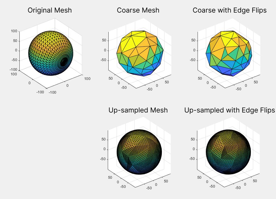
V.3. Preventing UV faces overlaps

According to Liu et al. 2020 [7], even with consistently oriented faces in the Euclidean and parameterized spaces, it is still possible that two faces overlap each other in the parameterized space. To prevent this artifact, the authors propose to check, in the UV domain, if an interior vertex of the edge to be collapsed has a total angle over \(2 \pi\). If this condition is satisfied, then the edge should not collapse. However, it may also be the case that the condition is satisfied after the collapse. In this case, this edge collapse must be undone and a different edge must be collapsed.

VI. Results

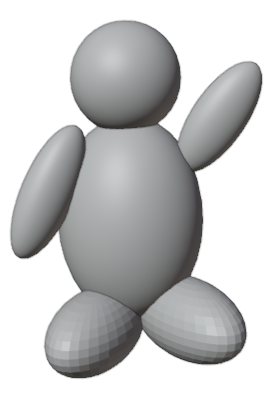
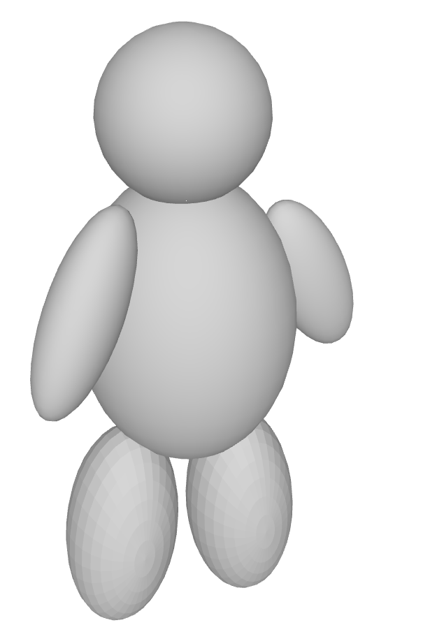
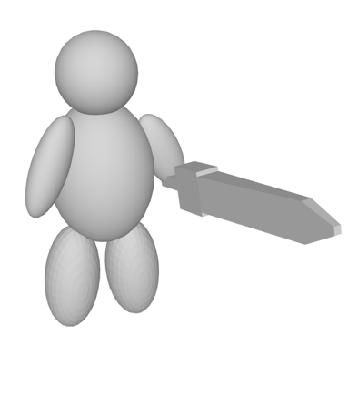
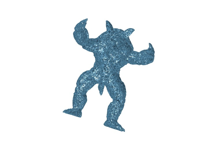
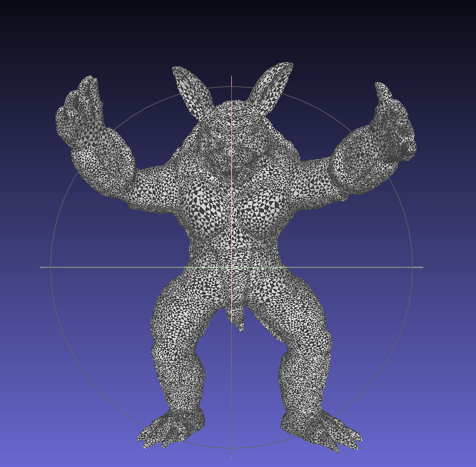
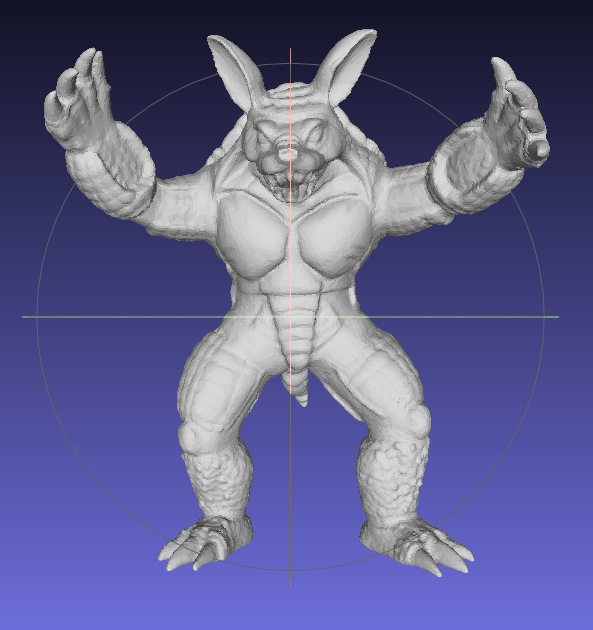
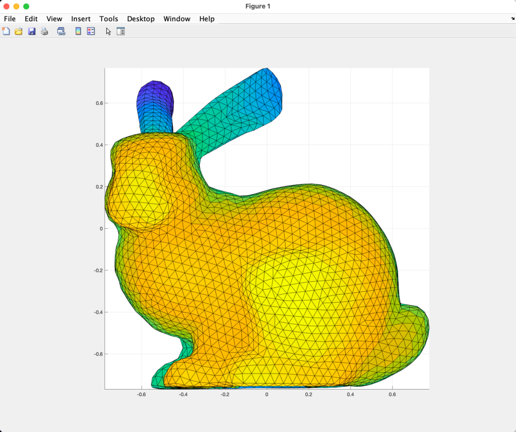
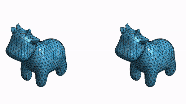
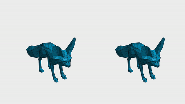
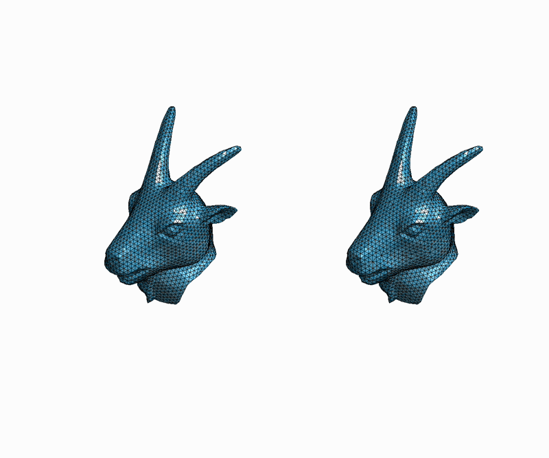
During this project we designed a procedure which can simplify any mesh via edge collapses as we have seen in all the animations. Figure 9 shows how well the coarse mesh approximates the original.

Figure 9: mean square distance between the original mesh and successive meshes in the hierarchy of meshes, built through mesh simplification.

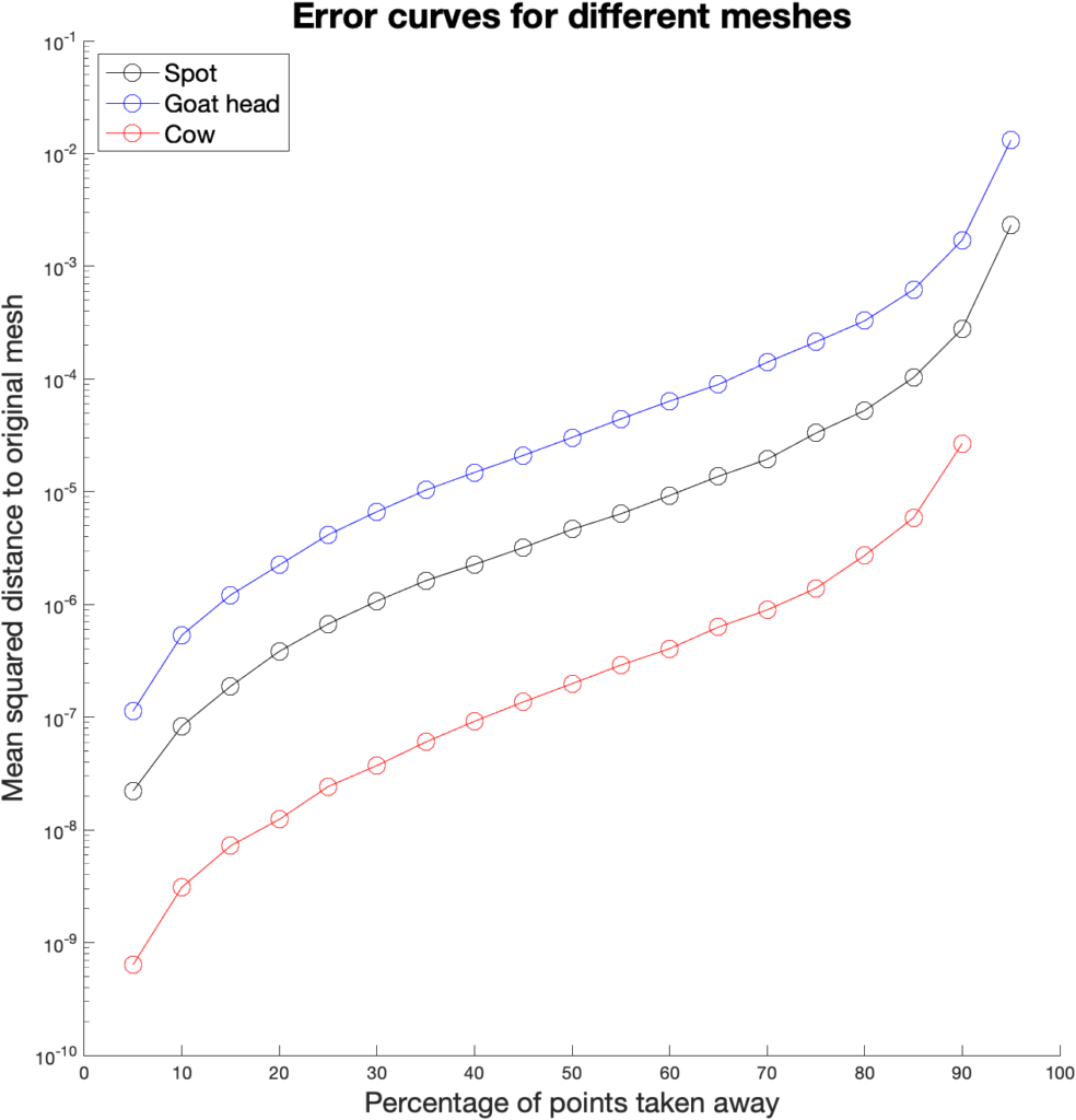
Another thing we measured was the quality of the mesh produced. Depending on the application, different measurements can be done. In our case, we have followed Liu et al. 2020 [7], which uses the quality measure \(Q_{ijk}\) defined in Section V.1. We average \(Q_{ijk}\) over all triangles in a mesh and plot the results across the percentage of vertices removed by edge collapses. Figure 10 shows the results for three different models.

Figure 10: variation of mean average quality along the hierarchy of meshes for three different models.

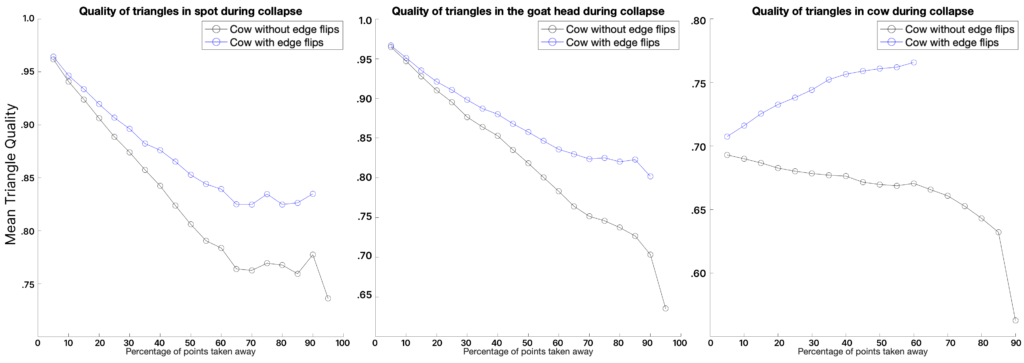
After the removal of approximately \(65 \%\) of the initial number of vertices, we notice that all meshes begin to level out and there is even marginal improvement for Spot the Cow model. Furthermore, we observe that the implementation of edge flips significantly increases the quality of the meshes produced. Unfortunately, we weren’t able to exploit its full capacity due to a lack of time and a bug in the code.

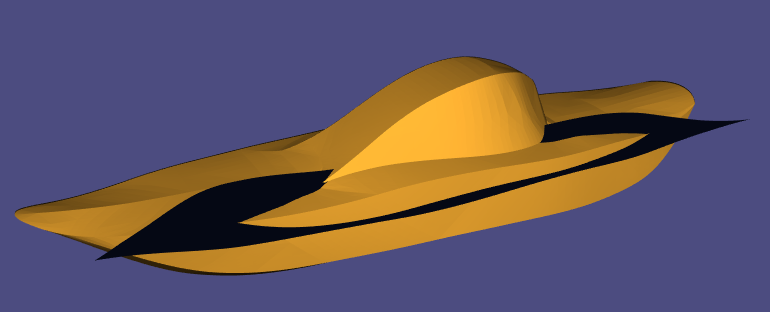
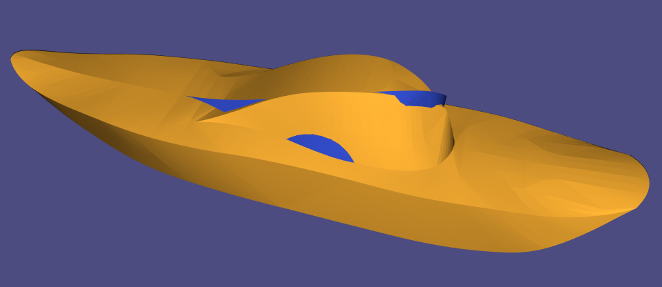
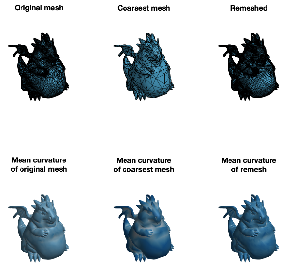
Finally, we have applied the self parameterization to perform remeshing. We have built a bijection \(\mathcal{M}^0\overset{f}{\longrightarrow}\mathcal{M}^L\) where \(\mathcal{M}^0\) is the coarsest mesh and \(\mathcal{M}^L\) is the original mesh. To remesh, we first upsample the topology of the coarse mesh \(M^{0}\), which adds more vertices and faces to the mesh. Subsequently, we use the bijective map to find correspondences between the upsampled mesh and the original mesh. With this correspondence, we build a new mesh with vertices lying inside the original. Figure 11 shows the result of the simplification followed by the remeshing process.

Figure 11: result of applying successive self-parameterization for remeshing. Given an initial fine mesh (left), it is simplified to a target number of faces (center). Then, this coarsest mesh is remeshed to match the original fine mesh (right). In the bottom row we can see the effect that this application has on the mean curvature.

VII. Conclusions and Future Work

In this project we explored hierarchical surface representations combined with successive self-parameterization, using mesh simplification to build a hierarchy of meshes and successive conformal mappings to build correspondences between different levels of the hierarchy. This allows to represent a surface with distinct levels of detail depending on the application. We investigated the application of the successive self-parameterization for remeshing and evaluated various quality metrics on the hierarchy of meshes, which provides meaningful insight into the preservation and loss of geometric data caused by the simplification process.

As main lines of future work, we envision using the successive self-parameterization to solve Poisson equations on curved surfaces, as done by Liu et al. 2021 [8]. While not yet complete, we started the implementation of the intrinsic prolongation operator, which is required for the geometric multigrid method to transfer solutions from coarse to fine meshes. Another step in this project could be creating a texture mapping between the course and fine mesh. Finally, another direction could be remeshing according to the technique using wavelets described in Khodakovsky et al. 2000 [1]. In this paper, wavelets are used to represent the difference between the coarsest and finest levels of a mesh.

While working on the application of Remeshing, that is, using the coarse mesh with upsampling and using the local information stored to reconstruct the geometry, we found that the edge flips after each collapse to be very promising. Based on that, we believe a more robust implementation of this idea can give better results in general. Moreover, we can use other remeshing operations when necessary. For example, tangential relaxation, edge splits and other operations might be useful for getting better-quality triangles. We have to be careful about how and when to apply edge splits, as applying them in each iteration would slow down the collapse convergence.

Another important line of work would be to improve performance and memory consumption in our implementation. While many operations were fully vectorized, there are still areas that can be improved.

We want to thank Professor Paul Kry for the guidance and mentorship (and patience on MATLAB debugging sessions) during these weeks. It is incredible how much can be learned and achieved in a short period of time with an enthusiastic mentor. We also want to thank the volunteers Leticia Mattos Da Silva and Erik Amézquita for all the tips and help they provided. Finally, we would like to thank Professor Justin Solomon for organizing SGI and making it possible to have a fantastic project with students and mentors from all over the world.

VIII. References

[1] Khodakovsky, A., Schröder, P., & Sweldens, W. (2000, July). Progressive geometry compression. In Proceedings of the 27th annual conference on Computer graphics and interactive techniques (pp. 271-278).

[2] Lee, A. W., Sweldens, W., Schröder, P., Cowsar, L., & Dobkin, D. (1998, July). MAPS: Multiresolution adaptive parameterization of surfaces. In Proceedings of the 25th annual conference on Computer graphics and interactive techniques (pp. 95-104).

[3] Mullen, P., Tong, Y., Alliez, P., & Desbrun, M. (2008, July). Spectral conformal parameterization. In Computer Graphics Forum (Vol. 27, No. 5, pp. 1487-1494). Oxford, UK: Blackwell Publishing Ltd.

[4] Lévy, Bruno, et al. “Least squares conformal maps for automatic texture atlas generation.” ACM transactions on graphics (TOG) 21.3 (2002): 362-371.

[5] Hoppe, H., DeRose, T., Duchamp, T., McDonald, J., & Stuetzle, W. (1993, September). Mesh optimization. In Proceedings of the 20th annual conference on Computer graphics and interactive techniques (pp. 19-26)

[6] Garland, M., & Heckbert, P. S. (1997, August). Surface simplification using quadric error metrics. In Proceedings of the 24th annual conference on Computer graphics and interactive techniques (pp. 209-216).

[7] Liu, H., Kim, V., Chaudhuri, S., Aigerman, N. & Jacobson, A. Neural Subdivision. ACM Trans. Graph.. 39 (2020)

[8] Liu, H., Zhang, J., Ben-Chen, M. & Jacobson, A. Surface Multigrid via Intrinsic Prolongation. ACM Trans. Graph.. 40 (2021)

[9] Levoy, M., Pulli, K., Curless, B., Rusinkiewicz, S., Koller, D., Pereira, L., Ginzton, M., Anderson, S., Davis, J., Ginsberg, J. & Others The digital Michelangelo project: 3D scanning of large statues. Proceedings Of The 27th Annual Conference On Computer Graphics And Interactive Techniques. pp. 131-144 (2000)

[10] Hormann, K., Lévy, B. & Sheffer, A. Mesh parameterization: Theory and practice. (2007)

[11] Li, W., Ray, N. & Lévy, B. Automatic and interactive mesh to T-spline conversion. 4th Eurographics Symposium On Geometry Processing-SGP 2006. (2006)

[12] Konaković, M., Crane, K., Deng, B., Bouaziz, S., Piker, D. & Pauly, M. Beyond developable: computational design and fabrication with auxetic materials. ACM Transactions On Graphics (TOG). 35, 1-11 (2016)

[13] Desbrun, M., Meyer, M. & Alliez, P. Intrinsic parameterizations of surface meshes. Computer Graphics Forum. 21, 209-218 (2002)

Categories
Research

Computational Design of Ship Models

Fellows: Ikaro Penha Costa, Bereket Faltamo, Sahana Kargi, Van Le

Advisor: Oded Stein, University of Southern California

Volunteers: Lucas Valenca, Shaimaa Monem

MOTIVATION

The art of assembling model kits has always been a fascinating hobby; however, the process of generating these models is often limited to surfaces that can be easily flattened. Traditionally, it takes the 3D artists weeks or even months to create a model with detailed instructions on how to assemble it. Thus, this research aims to explore the potential of developing a tool that can automate the process of capturing the curvature of more complex objects, allowing the construction of any given surface. Our ambitions are to offer professionals an unprecedented level of creative freedom by opening up the possibilities of replicating more intricate shapes and from there, pave the way for novel applications in the engineering world. 

METHODOLOGY

This project employs C++ and heavily uses the geometry processing library – libigl. For this research, the example objects are an icosahedron approximating the sphere and a mesh to a boat.

Segmentation into developable shapes

The first step is to determine whether it is a developable surface or not. In mathematics, a developable surface is a smooth surface with zero Gaussian curvature. We first took the boat and the icosahedral sphere and segmented them into parts that have zero Gaussian curvature. We checked the Gaussian curvature by using the Matlab code from Day 1 of the Tutorial Week. We could also do it with C++ by using this function.

Flattening pieces via corresponding homeomorphism

Once the shape is segmented, the next step is to flatten those segmented pieces. For this, we will use the geometry-processing-parameterization library and the Least Squares conformal mapping (LSCM) method. It works by finding and preserving the local angles and lengths between pieces. It aligns the centroids within the segments and then finds the optimal rotation, scaling, and translation using a least squares approach. Here are the results of implementing it on different segments of the boat.

Before LSCM After LSCM

In addition to flattening the pieces, we also colored them according to their coordinates. We normalized the X, Y, and Z coordinates of all the vertices and colored them the coordinating RGB color. The goal is to use this colormap during reassembly so that the flattened pieces can be curved to the proper amounts. 

Reassembling Pieces

In possession of the set of folded pieces, it naturally follows that each piece could be reconnected to revert this collection to the original object shape. This step is denominated reassembling instructions and essentially requires techniques of Shape Correspondence. That is, find a correspondence between a folded piece and the original shape.

Two main mathematical measures are involved in comparing the similarity of topological spaces: Hausdorff and Frechét distances. A more common implementation of bounds for Hausdorff distance is based on an energy optimization as discussed by Alec Jacobson in these tutorial notes. In this case, the Hausdorff distance is used to iteratively find the closest correspondence between a point in the source mesh and the entirety of the target mesh. This algorithm is Iterative Closest Point (ICP) and it is also available in libigl.

As seen in the image above, a segmented piece matches the correct place on the icosahedron after running the ICP algorithm. The ICP technique is, in summary, a sampling step of the mesh (VX, FX) and an optimization step in which each point in VX the objective function is to minimize the Hausdorff distance between this point and the target mesh (VY, FY).  The libigl provides the point-to-normal implementation discussed in Jacobson’s notes, which is a form of Gauss-Newton optimization algorithm. This method requires an integer for the number of sample points in (VX, FX) and also an integer for the maximum number of iterations to be used in the minimization algorithm.

The number of sample points and maximum iterations is decisive in order to obtain reliable reassembling results. As a common fact in optimization, depending on the number of iterations and size of the model, the algorithm might be susceptible to being stuck at a local minimum. This is also the case with ICP, causing artifacts as the image below:

A valid approach to avoid this sinister reassembling is to generate different initial conditions so that the optimization algorithm might converge to different local minima. In this case, using the Eigen library, a set of uniformly random rigid transformations are applied to the piece before passing it to the ICP method. Since the Hausdorff distance is the objective function, the rigid transformation which causes ICP to produce the lowest Hausdorff distance is stored and then used to produce the final result. 

However, research (and also life) is never linear. The approach described before would cause a few failed assertions throughout the label library. The assertions would be informed that the transformed mesh would have zero area. As the libigl area computation is robust, further investigations are necessary.

The investigations have determined the existence of overflow in the translation vector inside the ICP method. For the boat example, the entries in VX are originally in the magnitude of 101, and after some iterations of the ICP, the translation vector is applied to VX whose every entry would be numerically the same number in the magnitude of 1028; then, causing the transformed mesh to have zero area. In this case, the proposed remediation is to ignore the transformed initial pieces which would cause large entry-wise points in VX

Hence, after performing each ICP iteration with the extra care of managing the translation vector entries, promising results were found as shown in the image below. Observe that the piece matches a similar side of the boat but not the correct side, it is placed in the mirrored side. In this case, a possibility is that it might be necessary to add more constraints to the initial conditions. 

As finding the cause of zero areas has demanded significant time, the approach of adding more constraints to the initial conditions can be left as future work. For this, one can store information on the piece boundary in the segmentation step. This information could be used to point the ICP rotation and translation in the direction of the correct final place in the target shape at each iteration step. That is, try to point ICP rigid transformation to the original place of segmentation of each piece. Hopefully, this would cause correctness of results and faster convergence. 

Reassembling Instructions with Edge Coloring

When putting the pieces back together we need a way to know which parts come together. In particular, we need to know which pieces have shared edges. That is where edge coloring helps. We color-coded each cutting line with random patterns so that the pieces will take part of the pattern with them. The color coding of the icosahedron can be seen below. 

Icosahedron with Edge Coloring

Real Life Assembly by Adding Tabs and Holes 

As a final step, we wanted to see how accurate our algorithm was in real life. We formatted and printed the images and assembled them. Some work is needed in ensuring that all the individual shapes are the proper size. Additionally, we added the tabs and holes to the segments so the pieces fit together.

Final Boat Model

Link to Repo

ACKNOWLEDGEMENTS

We would like to express our sincere gratitude to Professor Oded Stein for his instruction, guidance, and encouragement throughout this research.

We would also like to acknowledge the advice and recommendations of the volunteers – Lucas and Shaimaa for offering help, unique insights, and perspectives. 

This research heavily used C++ and the library libigl.

Categories
Research

The (in)accurate Gradients of Neural Representations

Students: Gabriele Dominici, Daniel Perazzo, Munshi Sanowar Raihan, João Teixeira

TA: Nursena Koprucu

Mentors: Peter Yichen Chen, Rundi Wu, Honglin Chen, Ishit Mehta, Eitan Grinspun

1. Introduction

Implicit neural representation promises infinite resolution, automatic gradients, and memory efficiency. In practice, however, these promises often do not hold. Our project explored one specific drawback of implicit neural representations: the noisy gradient. The source code of this project is available on our GitHub repository.

The noisy gradient problem of neural representation has been observed in the context of solving PDEs [1], geometry processing [2,3], topology optimization [4], and 3D reconstruction [5].

1.1. Motivational Example: 1D advection

Our goal is to solve time-dependent PDEs on neural network-based spatial representations. Let’s consider the classic 1D advection equation:

This equation describes the passive advection of some scalar field u carried along at a constant speed a.

Fig 1: Advected scalar field (left), and gradient of the advected quantity (right) over time.

We will parameterize each time-discretized spatial field with a neural network. The field quantity at an arbitrary location can be queried via network inference f(x). The weights of this network are updated at each time step with optimization-based time integration [1]. 

1.2. The Problem: Noisy Gradients

   Fig 2: Comparisons of advected values and gradients of different neural representations. Ground truth (top row), the sine activation (middle row), and the Gaussian activation (bottom row).

Following the INSR literature, we explore different activation functions for our neural network-based scalar field. The figure above compares the predicted scalar quantity and their gradients for both sine [8] and Gaussian [12] activation networks. The predicted scalar quantity matches the ground truth well in all cases. But the gradient of the advected quantity is extremely noisy regardless of the choice of the activation function.

In the subsequent sections, we will tackle this problem using several approaches that fall into two categories: pure neural representation (Section 2) and hybrid grid-neural representations (Section 3).

2. Pure Neural Representations

2.1 Tuning Omega

Fig 3: Large omega values cause noisy gradients, while small omega values give smoother gradients.

The omega hyperparameter controls the frequency range that the SIREN network learns [8]. In general, if we reduce the value of omega, the gradients learned by the networks become less noisy. As seen in the figure above, choosing omega = 5 ensures the network has smooth gradients, while choosing a larger value like 50 gives us very noisy gradients. However, finding the optimal omega value is a non-trivial task. Users need to tune this parameter for each problem.

2.2. Finite Differences

Fig 4: Gradients estimated by finite difference method.

Instead of calculating the gradients by taking the derivative of the output with respect to the inputs using autodiff, we can also use finite differences to approximate the gradients. Because finite difference stencils have local compact supports, they are less susceptible to noise. Indeed, the gradients of the finite difference solution are much less noisy than the autodiff version (see figure above).

2.3 Averaging

Fig 5: Evolving of the gradient of the function over time in the mean gradients approach.

Instead of using the gradients computed by autodiff, we spatially average them by calculating the mean at four more neighboring points for each location.  Although the gradients seem smoother at the very beginning, it is easy to see that after a few timesteps, the gradient’s peaks become fictitiously taller, degrading the results (Fig 5). 

2.4 Initializing with Ground Truth Gradients

Fig 6: Evolving of the gradient of the function over time where the gradients are initialized to be the ground truth gradients.

At timestep 0, the neural network is trained to predict the initial values of the function we are trying to optimize. In addition, similarly to what is done in Sobolev training [6], we force the model to have the same gradients as the desired function. 

This method does reduce the noise in the gradient over time (Fig 6), but the information gathered from the extra supervision used in the initialization steps slowly dissolves. Furthermore, these gradients are not always available or not suitable for setting up a loss function in such a manner, making this solution not always applicable. 

3. Hybrid grid-neural representations

Fig 7: Description of the multi-resolution hashgrid (reproduced from [7]).

To address neural representations’ long training time, Muller et al. [7] developed a multi-resolution hash grid approach: instantNGP. In the following section, we explore instantNGP’s gradient quality. We benchmark it on a 2D fluid example. The figure below shows the example’s initial condition:

Fig 8: Vortex velocity field (reproduced from [1]).

When we try to fit this initial condition using a pure neural representation (i.e., NOT instantNGP), we observe highly noisy gradients, consistent with the results reported in Section 2.1.

Fig 9: Gradient we obtained using pure neural representations for the proposed 2D vortex problem.

Next, we investigated hybrid neural-grid representations, varying the type of the grids and the type of the hash (See Fig 10). 

Fig 10: Different gradients for different resolutions.

The parameters outlined in green obtained the best result. In this case, we use a base resolution of 256 and a 3-level hash grid. 

However, those results only accounted for the initial conditions. If we let the gradients evolve for 99 timesteps according to the PDE, we observe that the gradients start diverging, as can be seen in the video below.

Fig 11: Evolution of the gradients for the 2D fluids for the two vortices example. This test was done with a dense grid of 512 resolution.

In summary, although our hybrid approach seems excellent for the first timesteps, it also appears to limit the expressivity of the network during subsequent evolution.

Due to these problems in the 2D Fluid scenario, we investigated the gradients’ performance in another environment: the 2D Advection problem.

Fig 12: Comparison of Gradient Magnitudes for Different methods.

We used the same network configurations (base resolution, number of levels, number of hidden layers, and hidden features) as the 2D Fluid problem. The hybrid neural-grid representation performs significantly worse than the pure neural representation using SIREN (see Fig 12). Here the network is asked to fit the initial condition only.

Next, we tried to tune the configuration parameters. We discovered that the models performed better for the 2D Advection scenario when the number of level is increased. The best result is given by the following parameters:  number of Levels: 16; per Level Scale: 1.5; Base resolution: 16.

Fig 13: Comparison of Gradient Magnitudes for Hash grid’s best parameters.

Even though the hash grid’s performances improved, the figure above demonstrates that the gradients are still much noisier than the pure neural representation (SIREN). 

As such, we conclude that the hybrid grid-neural representation’ performance is not consistently better than the pure neural representation. In fact, it’s sometimes worse, as demonstrated in the 2D advection example.

4. Future Work

Since our tests and other SIREN works [8] show that tuning the omega hyperparameter is essential for the gradient results, one possible next step is to perform automatic gradient tuning, as proposed in meta-learning techniques [9].

Another possible approach is supervising the gradients. Instead of using the original function to compute the gradients, it is possible to use a separate loss function that certifies the correct gradient values over time. Essentially, we aim to write down the evolution equation of the gradient itself and couple this equation with the original PDE.

Future work should also consider a theoretical understanding of the gradient problem. One possible cause for this problem is the global non-compact support of neural networks. This initially motivates us to explore hybrid grid-neural networks. Other works [7, 10, 11] used similar approaches to extract local features to feed into the network, enforcing a locality to the neural network.

5. References

[1] Chen, Honglin, Wu Rundi, Eitan Grinspun, Changxi Zheng, and Peter Yichen Chen. “Implicit Neural Spatial Representations for Time-dependent PDEs.” International Conference on Machine Learning (ICML). 2023.

[2] Mehta, Ishit, Manmohan Chandraker, and Ravi Ramamoorthi.” A level set theory for neural implicit evolution under explicit flows.” European Conference on Computer Vision (ECCV).  2022.

[3] Yang, Guandao, Serge Belongie, Bharath Hariharan, and Vladlen Koltun. “Geometry processing with neural fields.” Neural Information Processing Systems (NeurIPS). 2021.

[4] Zehnder, Jonas, Yue Li, Stelian Coros, and Bernhard Thomaszewski. “Ntopo: Mesh-free topology optimization using implicit neural representations.” Neural Information Processing Systems (NeurIPS). 2021.

[5] Verbin, Dor, Peter Hedman, Ben Mildenhall, Todd Zickler, Jonathan T. Barron, and Pratul P. Srinivasan. “Ref-nerf: Structured view-dependent appearance for neural radiance fields.” Conference on Computer Vision and Pattern Recognition (CVPR).  2022.

[6] Czarnecki, Wojciech M., Simon Osindero, Max Jaderberg, Grzegorz Swirszcz, and Razvan Pascanu. “Sobolev training for neural networks.” Neural Information Processing Systems (NeurIPS). 2017.

[7] Müller, Thomas, Alex Evans, Christoph Schied, and Alexander Keller. “Instant neural graphics primitives with a multiresolution hash encoding.” ACM Transactions on Graphics (ToG) 41. 2022.

[8] Sitzmann, Vincent, Julien Martel, Alexander Bergman, David Lindell, and Gordon Wetzstein. “Implicit neural representations with periodic activation functions.” Neural Information Processing Systems (NeurIPS). 2020.

[9] Hospedales, Timothy, Antreas Antoniou, Paul Micaelli, and Amos Storkey. “Meta-learning in neural networks: A survey.” IEEE transactions on pattern analysis and machine intelligence 44.9. 2021.

[10] Sun, Cheng, Min Sun, and Hwann-Tzong Chen. “Direct voxel grid optimization: Super-fast convergence for radiance fields reconstruction.” Conference on Computer Vision and Pattern Recognition (CVPR). 2022.

[11] Barron, Jonathan T., Ben Mildenhall, Dor Verbin, Pratul P. Srinivasan, and Peter Hedman. “Zip-NeRF: Anti-aliased grid-based neural radiance fields.”  International Conference on Computer Vision (ICCV). 2023.

[12] Shin-Fang Chng, Sameera Ramasinghe, Jamie Sherrah, Simon Lucey. “Gaussian Activated Radiance Fields for High Fidelity Reconstruction and Pose Estimation” The European Conference on Computer Vision (ECCV). 2022.

Categories
Research

Exploring Temporal Consistency and Cross-Modal Interaction of Latent NeRF

Authors: Sana Arastehfar, Erik Ekgasit, Berfin Inal, Maria Stuebner

Abstract:

Latent NeRF (Neural Radiance Fields) is a state-of-the-art generative model capable of synthesizing 3D-consistent 2D images from a combination of 3D-sketch and text guides. In this report, we investigate the temporal consistency of Latent NeRF by generating 3D-consistent images with different sketch guides and exploring the interplay between 3D-sketch guidance and text prompts in the generation process; with a broader motivation of using diffusion models in animation and dynamic scene generation. Through our experiments, we discover the importance of incorporating both 3D sketch and text information to achieve accurate and consistent results. Additionally, we propose potential enhancements, including the integration of geometry/shape loss and automatic generation of descriptive text from geometry, to improve the model’s performance.

Introduction:

Neural Radiance Field (NeRF) is a relatively new representation of geometry. They use a neural network to approximate a function F: (x, θ) → (c, σ) that can model the appearance of a single scene. This function takes a sampled input 3D point x and a viewing direction θ derived from a 2D image (with camera information) and returns the color c = (r, g, b) and volume density σ of the shape at that point. This is enough to encode the shape and color of a scene as well as view-dependent lighting effects in the scene with a radiance field.

Traditionally, NeRFs have been trained with sets of images from the real world or images that are rendered using computer graphics software. Recently, image diffusion models such as Stable Diffusion have been able to generate coherent images from just text prompts. Combining diffusion models and NeRFs has led to Latent NeRF, a cutting-edge generative model that uses an image diffusion model to train NeRFs using just a text prompt and an optional guiding 3D shape.

We investigate the use of latent-nerf to create sequential images and animation. One major challenge in doing so is temporal consistency. It is currently challenging to ensure that diffusion models recreate the same object/character between runs. This week, we attempt to achieve temporal consistency of the model’s output and the influence of combining different input modalities.

Methodology:

We conducted a series of experiments to evaluate the temporal consistency of the Latent NeRF model and explore the interaction between sketches and text prompts during image synthesis.

Temporal Consistency Assessment:

We first decided to test consistency between two poses under the most naive approach to get a baseline for consistency in latent-nerf. We started by using sketch shapes to guide the shape of the NeRFs. Each sketch shape is a collection of simple triangle meshes arranged in roughly the same shape as the desired output. Our Blender-master of the team, Erik, created sketch shapes of a teddy bear in different poses and configurations to guide the NeRF generation. Figure 1 depicts the original sketch-shape of a teddy bear with its left arm raised, and Figure 2 shows the same teddy bear sketch with both arms down. Given the same text prompt, would the NeRFs generated from these sketch shapes look like the same object in different poses? According to the results in Figure 4 and Figure 5, the answer is no. The models have different colors, making them unsuitable to use as frames of animation.

Figure 1: Default teddy bear sketch with left arm up
Figure 2: Teddy bear sketch with both arms down
Figure 3: Teddy bear sketch holding a sword
Figure 4: Teddy with right arm up (default in Figure 1) sketch with the text prompt ‘a lego man’
Figure 5: Teddy with both hands down sketch (Figure 2) with the text prompt ‘a lego man’

Cross-Modal Interaction:

To understand the interplay between sketches and text prompts, we augmented the base sketch with a sword (Figure 3). We experimented with two different text prompts: “a lego man” (since this is the convention in previous papers to call it a “lego man” instead of a “lego human”) and “a lego man holding a sword”. Figure 6 illustrates the output when using the “a lego man” text prompt, which resulted in only the phantom of the sword being generated. However, when using the “a lego man holding a sword” text prompt, the model successfully generated a visible sword (Figure 7). The presence of both image and text prompts is crucial for generating visible new objects, suggesting the importance of cross-modal interaction.

Figure 6: Teddy holding a sword sketch with the text prompt ‘a lego man’
Figure 7: Teddy holding a sword sketch with the text prompt ‘a lego man holding a sword’

Additionally, we wanted to assess the level of support required from sketch-guidance while using text-guidance. To test this, we generated various lego humans based on specific instructions, such as ‘a lego man with right arm up’, ‘a lego man with left arm up’, while keeping the sketch guidance consistent with the same teddy sketch in Figure 1. As seen in Figures 8 and 9, despite the text prompts requesting opposite actions, the outputs are quite similar to each other, suggesting that text-guidance itself is not sufficient to generate the desired output.

Figure 8 : Default teddy sketch (Fig. 1) with the text prompt ‘a lego man with right arm up’
Figure 9: Default teddy sketch (Fig. 1) with the text prompt ‘a lego man with left arm up’
Discussion:

Our observations indicate that Latent NeRF’s temporal consistency can be improved by incorporating additional constraints and interactions between different input modalities. This suggests that using a long description of the desired character could enforce temporal consistency between poses.

Ideas:

Building on our observations and discussions, we have some ideas as to how to improve temporal consistency in Latent-NeRF. We could integrate a geometry/shape loss to enhance the model’s ability to maintain consistency between generated images. Additionally, we could develop a mechanism to automatically extract descriptive word descriptors from geometry to use as complementary text prompts. Finally, we could use Stable Diffusion concepts to guide consistency.

Potential Experiments:

Moving forward, we would like to explore the consistency in generating objects with similar geometry (e.g., different keywords as, sword, stick, etc. with the same sketch). To that end, we plan to repeat the same experiment, but with different combinations of geometry and text. Additionally, we would like to investigate the model’s performance when utilizing text prompts unrelated to the geometry, such as “stick” or “apple,” (when the sketch, in fact, displays a sword) to evaluate the robustness of cross-modal interactions. Lastly, we think it would be interesting to find/create a Stable Diffusion concept and apply it to the generation of two different poses.

Conclusion:

Our exploration of Latent NeRF’s temporal consistency and cross-modal interactions highlights the importance of combining sketch and text guides to achieve consistent and accurate 3D image synthesis. By addressing the observed issues and implementing potential enhancements, the model can be further refined to generate even more realistic and consistent images across different inputs. Eventually, this will help animators, modelers, and content creators to easily generate dynamic NeRFs with articulated characters and scenes.

Technical Journey:

Neural networks are renowned for their substantial computational demands, leading to extended training and inference times. Despite notable advancements in the realm of NeRFs research, which have contributed to improved training and inference speeds, these models continue to exhibit high memory requirements. Similarly, diffusion models also exhibit a pronounced appetite for memory resources. Consequently, the execution of Latent-NeRF necessitates access to machines equipped with GPUs boasting a minimum of 12 GB of VRAM.

The training of a single NeRF entails a substantial time investment, ranging from 30 minutes when using NVIDIA RX 3090 to 3 hours using Google Colab. Moreover, the implementation of latent NeRF entailed the integration of numerous dependencies, a process that demanded considerable troubleshooting efforts to ensure proper installation. Given the convergence of the two distinct areas of graphics research, namely NeRFs and Diffusion models, encountering technical challenges during dependency management was a foreseeable aspect of the endeavor. Such technical trouble shooting constitutes an inevitable and crucial facet of the overall research process.

Fortunately, the mentors of this project Sainan Liu, Ilke Demir and Olga Guțan, provided valuable guidance in navigating these technical complexities, which significantly expedited the resolution of issues and allowed us to focus more efficiently on the core aspects of our project.

Papers:

For temporal consistency with better texture/geometry details we explored: D-nerf, EditableNeRF, Tetra NeRF, NeRFEditing, One-2-3-45. For gometric manipulation for temporal consistent 3D animation generation with text/image guidance, SKED and DASR were reviewed.

Categories
Tutorial week

Last Day of SGI 2023 Tutorial Week

After many exercises, lectures, presentations, and MATLABs abruptly closing, we reached the end of the first week of SGI 2023. It was a wild and incredible ride. And we reach the end with a course by Nicholas Sharp on Robustness in Geometry Processing. We also had a guest lecture by Teseo Schneider and, finally, our release of the projects for the next week. Having this experience while in my home city of Recife, Brazil is incredible.

In Sharp’s presentation, we learned that meshes extracted from real data are much less clean than ideal meshes. So, we must create techniques and methods to perform robust geometry processing. In the first part, we learned about floating point arithmetic. We learned that contrary to what we programmers want to think, floating point numbers are NOT real numbers and can introduce many errors during arithmetic. For example, we learned that there are better ideas than performing a strict equality comparison and that we should add a tolerance factor to account for errors.

We also got an introduction to different numerical solvers and how meshes with some properties can break numerical solvers. Although these properties can result from error, sometimes they are intentional. As an example of such properties that can break processing, meshes can have:

  • Duplicate Vertices
  • Faces of wrong orientation
  • Can be nonmanifolds
  • And many more

To get a feeling of how to perform different processing methods, we did some activities on how to do processing with “bad meshes” Those activities are available here. One such example was an activity on bad meshes. For example, we were given a “bad_armadillo”, a variation of the traditional armadillo mesh that, when loaded, looked odd:

To correct this issue, we used Meshlab. When we loaded it into Meshlab, it became clear that some normals were inverted:

So, after orienting the meshes to the right side, we “fixed the mesh”:

And now MATLAB can load it the proper way.

We also got a presentation by Professor Teseo Schneider of the University of Victoria on their work on collision detection. Their technique could simulate different structures such as chains, arches, dimensional card houses, and even a cube rotating in a turntable with varying friction parameters. To end the lecture, he showed a really satisfying simulation of a stack of bricks being hit by a wrecking ball (Figure taken from his paper, available here):

Finally, at the end of the day, we got the list of the projects we will work on next week. I was paired with many amazingly talented fellow students (one of them is also Brazilian like me!) to work on a project on Hybrid Neural and Grid Representations, mentored by Peter Chen. I can’t wait for what SGI 2023 has in store!

Categories
Tutorial week

First Day of Summer Geometry Initiative 2023

The opening day of the MIT Summer Geometry Initiative 2023 was filled with engagement as the students dived into the world of geometry.

The program kicked off with Dr. Solomon welcoming the 2023 SGI Fellows and provided basic information on how the week will go.

It was followed by Dr. Oded Stein’s course introducing the basic techniques in geometry processing using the gptoolbox library. His talk started with a review of the basic concepts of geometry from the perspectives of different people who might use it. Dr. Stein also introduced the students to some advanced topics, such as how to store surfaces on a computer and how to define the boundary of a surface. The students were given various MATLAB exercises to experiment with the ideas he talked about.

In the afternoon, we had a guest lecture from Dr. Vladmir (Vova) Kim at Adobe, who spoke on the applications of geometry processing. He explained how geometry processing can be used to manipulate shapes in different ways, such as deformation, using neural progressive meshes and parameterization. The methods he introduced can be applied to computer graphics and computer vision. The lecture provided us with a glimpse into state-of-the-art in this cutting-edge field.

Overall, the first day of the MIT Summer Geometry Initiative 2023 was a resounding success. The students left with a solid foundation in geometry processing, ready to tackle more advanced topics in the days ahead.

Categories
Logistics

Welcome to SGI 2023!

Welcome to the official blog of the Summer Geometry Initiative (SGI) 2023, taking place July 10-August 18! I’m Justin Solomon, director of SGI 2023 and PI of the MIT Geometric Data Processing Group.

First launched in 2021, SGI is a completely online program engaging a paid cohort of undergraduate and early master’s students in six weeks of training and research experiences related to applied geometry and geometry processing. SGI Fellows come from all over the globe and represent a wide variety of educational institutions, life/career paths, and fields of interest.

SGI aims to accomplish the following objectives:

  • spark collaboration among students and researchers in geometry processing,
  • launch inter-university research projects in geometry processing involving team members across broad levels of seniority (undergraduate, graduate, faculty, industrial researcher),
  • introduce students to geometry processing research and development, and
  • diversify the “pipeline” of students entering geometry processing research, in terms of gender, race, socioeconomic background, and home institution.

SGI aims to address a number of challenges and inequities in geometry processing. Not all universities host faculty whose work touches on this emerging field, reducing the cohort of students exposed to this discipline during their undergraduate careers. Moreover, as with many engineering and mathematical fields, geometry processing suffers from serious gender, racial, and socioeconomic imbalance; by giving a broad set of students access to geometry processing research experiences, over the longer term we hope to affect the composition of the geometry processing community.

SGI is supported by a worldwide network of volunteers, including faculty, graduate students, and research scientists in geometry and related disciplines. This team supports the SGI Fellows through mentorship, instruction, panel discussions, and several other means.

SGI 2023 is due to start in a few days! Each SGI Fellow has been mailed a box of swag from our many sponsors, a certificate, and a custom-made coffee mug designed by SGI 2023 Fellows Hossam Saeed, Biruk Abere, Daniel Perazzo, and others.

We’ll kick off next week with tutorials in geometry processing led by Oded Stein (MIT), Silvia Sellán (U of Toronto), Jiayi Eris Zhang (Stanford), Michal Edelstein (Technion), and Nick Sharp (NVIDIA). Then, in the remaining 5 weeks, our Fellows will have the opportunity to participate in multiple short-term (1-2 week) research projects, intended to kick off collaborations that last over the longer term. Check out last year’s SGI blog for examples of the kinds of projects they’ll be working on.

Revisit this blog as the summer progresses for updates on SGI 2023 and to read about the exciting ideas our Fellows are developing in geometry!