Students: Daniel Perazzo, Sanowar Munshi, Francheska Kovacevic
TA: Kevin Roice
Mentors: Antonio Teran, Zachary Randell, Megan Williams
Introduction
Monitoring the health and sustainability of native ecosystems is an especially pressing issue in an era heavily impacted by global warming and climate change. One of the most vulnerable types of ecosystems for climate change are the oceans, which means that developing methods to monitor these ecosystems is of paramount importance.
Inspired by this problem, this SGI 2023 project aims to use state-of-the-art 3D reconstruction methods to monitor kelp, a type of algae that grows in Seattle’s bay area.
This project was done in partnership with Seattle aquarium and allowed us to use data available from their underwater robots as shown in the figure below.
Figure 1: Underwater robot to collect the data
This robot collected numerous pictures and videos in high-resolution, as seen in the figure below. From this data, we managed to perform the reconstruction of the sea floor, by some steps. First we perform a sparse reconstruction to get the camera poses and then we perform some experiments to perform the dense reconstruction. The input data is shown below.
Figure 2: Types of input data extracted by the robot. High-resolution images for 3D reconstruction
Sparse Reconstruction
To get the dense reconstruction working, we first performed a sparse reconstruction of the scene, in the image below we see the camera poses extracted using COLMAP [5], and their trajectory in the underwater seafloor. It should be noted that the trajectory of the camera differs substantially from the trajectory of the real robot. This could be caused by the lack of a loop closure during the trajectory of the camera.
Figure 3: Camera poses extracted from COLMAP.
With these camera poses, we can reconstruct the depth maps, as shown below. These are very good for debugging, since we can visualize and get a grasp of how the output of COLMAP differs from the real result. As can be seen, there are some artifacts for the reconstruction of the depth for this image. And this will reflect in the quality of the 3D reconstruction.
Figure 4: Example of depth reconstruction using the captured camera poses extracted by COLMAP
3D Reconstruction
After computing the camera poses, we can go to the 3D reconstruction step. We used some techniques to perform 3D reconstruction of the seafloor using the data provided to us by Dr. Zachary Randell and his team. For our reconstruction tests we used COLMAP [1]. In the image below we present the image of the reconstruction.
Figure 5: Reconstruction of the sea-floor.
We can notice that the reconstruction of the seabed has a curved shape, which is not reflected in the real seabed. This error could be caused by the fact that, as mentioned before, this shape has a lack of a loop closure.
We also compared the original images, as can be seen in the figure below. Although “rocky”, it can be seen that the quality of the images is relatively good.
Figure 6: Comparison of image from the robot video with the generated mesh.
We also tested with NeRFs [2] in this scene using the camera poses extracted by COLMAP. For these tests, we used nerfstudio [3]. Due to the problems already mentioned for the camera poses, the results of the NeRF reconstruction are really poor, since it could not reconstruct the seabed. The “cloud” error was supposed to be the reconstructed view. An image for this result is shown below:
Figure 7: Reconstruction of our scene with NeRFs. We hypothesize this being to the camera poses.
We also tested with a scene from the Sea-thru-NeRF [4] dataset, which yielded much better results:
Figure 8: Reconstruction of Sea-thru-NeRF with NeRFs. The scene was already prepared for NeRF reconstruction
Although the perceptual results were good, for some views, when we tried to recover the results using NeRFs yielded poor results, as can be seen on the point cloud bellow:
Figure 9: Mesh obtained from Sea-thru-NeRF scene.
As can be seen, the NeRF interpreted the water as an object. So, it reconstructed the seafloor wrongly.
Conclusions and Future Work
3D reconstruction of the underwater sea floor is really important for monitoring kelp forests. However, for our study cases, there is a lot to learn and research. More experiments could be made that perform loop closure to see if this could yield better camera poses, which in turn would result in a better 3D dense reconstruction. A source for future work could be to prepare and work in ways to integrate the techniques already introduced on Sea-ThruNeRF to nerfstudio, which would be really great for visualization of their results. Also, the poor quality of the 3D mesh generated by nerfstudio will probably increase if we use Sea-ThruNeRF. These types of improvements could yield better 3D reconstructions and, in turn, better monitoring for oceanographers.
References
[1] Schonberger, Johannes et al. “Structure-from-motion revisited.” IEEE Conference on Computer Vision and Pattern Recognition (CVPR). 2016.
[2] Mildenhall, Ben, et al. “Nerf: Representing scenes as neural radiance fields for view synthesis.” Communications of the ACM. 2021
[3] Tancik, M., et al. “Nerfstudio: A modular framework for neural radiance field development”. ACM SIGGRAPH 2023.
[4] Levy, D., et al. “SeaThru-NeRF: Neural Radiance Fields in Scattering Media.” IEEE/CVF Conference on Computer Vision and Pattern Recognition (CVPR). 2023.
[5] Schonberger, Johannes L., and Jan-Michael Frahm. “Structure-from-motion revisited.” IEEE/CVF Conference on Computer Vision and Pattern Recognition (CVPR). 2016.
By Aditya Abhyankar, Biruk Abere, Francisco Unai Caja López and Sara Ansari
Mentored by Kartik Chandra with help from the volunteer Shaimaa Monem
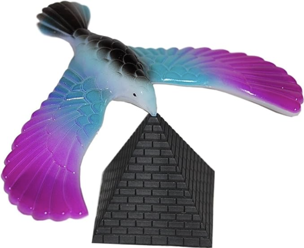
In this project we are looking for ways to generate physical illusions. More to the point, we would like to generate objects that, similarly to this bird, can be balanced in a surprising way with just one support point. To do this we have considered both the physics of the system and we draw on theories from cognitive science to model human intuition.
1. Introduction
Every day in your life, you make thousands of intuitive physical judgements without noticing. ‘Will this pile of dishes in the sink fall if I move this cup?’, ‘If it does fall, in which way will it fall?’ The judgements we make are accurate in most scenarios, but sometimes mistakes happen. Just like how occasional errors in vision lead to visual illusions (e.g. the dress and the Muller-Lyer illusion) occasional errors in intuitive physics should lead to physical illusions. To generate new illusions, there are two steps that could be followed.
First, we could design a method that appropriately models the way people make intuitive judgements based on their perception of the world. In that regard it’s interesting to read [1] which models intuitive physical judgement via physical simulations.
Secondly, we could try to ‘fool our model’ or to find an adversarial example. That is, find a physical scenario in which the output of the model is wrong. If the model is appropriately chosen, the results may also fool humans, thus producing new physical illusions. This approach has been used in [2] to generate images with properties similar to the dress.
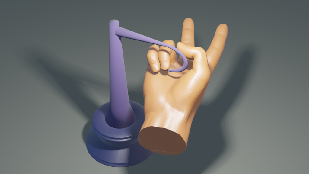
In this project we aim to find a different kind of illusion. Consider the following toy (image from Amazon). Many people would guess that the bird would fall if it’s only supported by its beak.
However, the toy achieves a perfectly stable balance in that position. We seek to find other objects that behave similarly: they achieve stable balance given a single support point even when many people guess that it is going to fall.
2. Physical stability vs intuitive stability
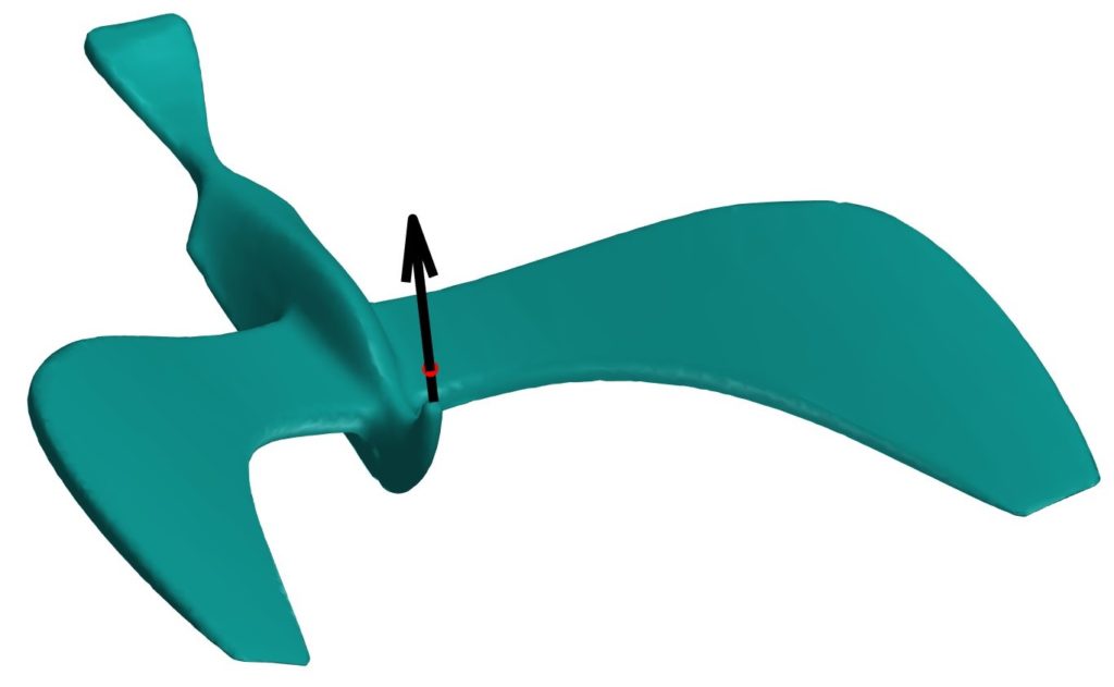
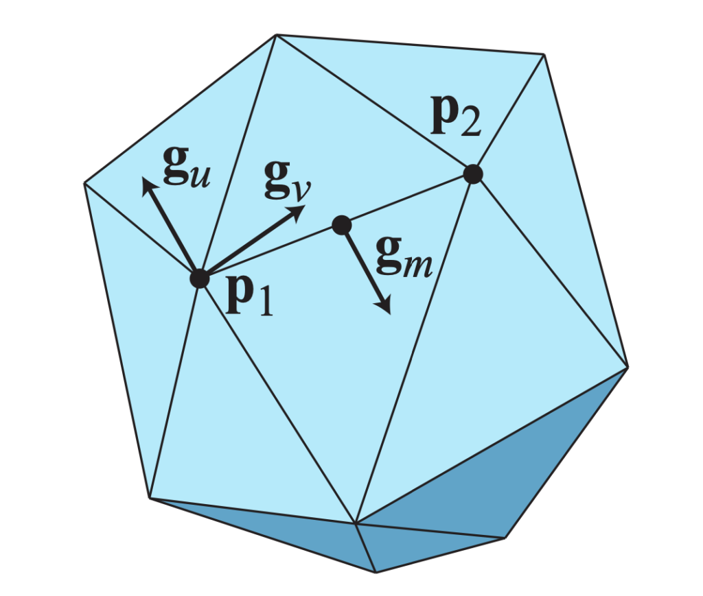
Consider a frictionless rigid body with uniform density and a point p on its boundary with unit normal n. For the object to balance at p, its normal n must point ‘downwards’ in the direction of gravity, for otherwise it will slide. Perfect balancing will then be achieved if the line connecting p and the object’s volumetric center of mass (COM) m is parallel to n. This can be achieved for the balancing bird when the point p is the beak as can be approximately seen in the following figure (mesh obtained from thingiverse). Here we have the center of mass in red and the vector showing the direction of m−p.
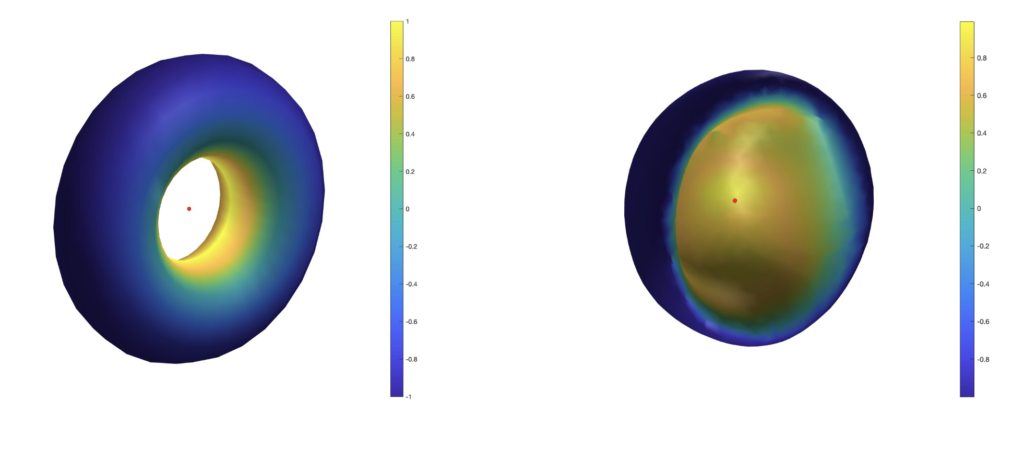
Since an object can always be rotated so that n points downwards, the quality of the balancing can be assessed by the evaluating the dot product (m−p) · n. To be precise, we use the normalized vectors to compute the dot product. The greater this value, the more stable the balancing at p. If m−p and n are parallel and have the same direction, then a perfect balancing will be achieved, and it will be stable. If they are parallel with opposite direction, a perfect balancing will still be achieved, but it will be unstable; i.e. small perturbations will make it fall. Points with dot product values in between will lie somewhere on a spectrum of stability, determined by their dot product’s closeness to the positive extremum. To illustrate this concept, we have taken a torus and a ‘half coconut’ mesh and plotted the dot product of normalized m−p, n. The center of mass appears in red.
There is some evidence [4] that humans asses a rigid body’s ability to stably balance at a point in a very similar way. The only difference is that instead of considering the object’s actual COM, whose location can be counterintuitive even with uniform density, humans judge stability based on the COM mch of the object’s convex hull. Thus to find an object that stably balances in a way that looks counterintuitive to humans, we must search for objects with at least one boundary point p such that (m−p) · n is maximized, but (mch−p) · n is minimized.
In general, to compute the center of mass of a region M⊂ℝ3, we would need to compute the volume integral
where ρ is the density of the object. However, for watertight surfaces with constant density, this volume integral can be turned into a surface integral thanks to Stokes’ theorem. Therefore, the center of mass can be computed even if we only know the boundary of the object, which for us is encoded as a triangle mesh. The interested reader learn more about this computation in [3].
3. Finding new illusions
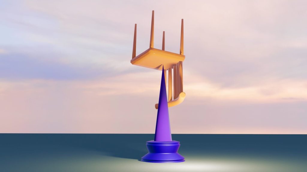
Given a mesh, one simple way to find new illusions would be to look for a vertex p such that (m−p) · n is positive and close to its maximum, while (mch−p) · n is as small as possible (again, we will use normalized versions of the vectors). Of course, these are two conflicting tasks. In this project we have chosen to maximize a function of the form
where w is a weight. By increasing w, we are more likely to find points were m−p and n are almost parallel, which is desirable to achieve a stable balance. The most interesting results were found when (m−p) · n ≈ |m−p| and (mch−p) · n < 0.7|mch−p|. For instance, we have the following chair.
This chair is part of the SHRECK 2017 dataset. We also examined some meshes from Thingi10k and one of the results was the following.
In the previous pictures, assuming constant density, each object is balanced with only one support point. Finally, we have the following hand which can be found in the Utah 3D Animation Repository.
4. Results and future work
Here we list some limitations of our project and ways in which they could be overcome.
Are we certain that the results obtained really fool human judgement? Our team finds these balancing objects quite surprising or, at the very least, aesthetically pleasing. We could try giving more definite proof by designing a survey. For example, people could look at different objects supported at a single point and guess if the objects would fall or not.
We have only verified that the objects should be stably balanced by computing the location of the center of mass. We could further test this by running physical simulations and by 3-D printing some of the examples.
Given a 3-D object that has already been modeled. We checked whether it could be balanced in any surprising way. One step forward would be generating 3-D models of objects that verify the properties we desire. It would be desirable that given a mesh (e.g. of an octopus), we could deform it so that the result (which hopefully still looks like an octopus) can be balanced in a surprising way.
5. Conclusion
Let’s take a step back and see this project has taught us. We started with the question: why do some objects, like the balancing bird, seem so surprising? This led us to study how people perceive objects through their center of mass and, after searching through a variety of 3D data sets, we found objects that also seem to balance in a surprising way. This was a very fun project and we really enjoyed it as a group, it involved playing with a bit of math, the geometry of triangle meshes and making beautiful visualizations while also learning something about human perception. Finally, we would like to thank Justin Solomon for organising the SGI, giving us this wonderful opportunity and Kartik Chandra for offering and mentoring such a fun project.
References
[1] Peter W Battaglia, Jessica B Hamrick, and Joshua B Tenenbaum. Simulation as an engine of physical scene understanding. Proceedings of the National Academy of Sciences, 110(45):18327–18332, 2013.
[2] Kartik Chandra, Tzu-Mao Li, Joshua Tenenbaum, and Jonathan Ragan-Kelley. Designing perceptual puzzles by differentiating probabilistic programs. In ACM SIGGRAPH 2022 Conference Proceedings, pages 1–9, 2022.
[3] Brian Mirtich. Fast and accurate computation of polyhedral mass properties. Journal of graphics tools, 1(2):31–50, 1996.
[4] Yichen Li, YingQiao Wang, Tal Boger, Kevin A Smith, Samuel J Gershman, and Tomer D Ullman. An approximate representation of objects underlies physical reasoning. Journal of Experimental Psychology: General, 2023.
By Gizem Altintas, Biruk Abere Ambaw, Francheska Kovacevic, Emi Neuwalder
During the first week of SGI, we worked with Prof. Yusuf Sahillioglu and Devin Horsman to explore convex geometry and some of the 3D decomposition techniques.
1. Introduction:
3D convex decomposition refers to a computational technique that breaks down a 3D object (usually represented as a mesh) into smaller convex sub-components. It is a popular computational process in computer graphics, computational geometry, and physics simulations. In other words, the objective of a 3D convex decomposition is to divide a complicated 3D object into a collection of simpler, non-overlapping convex shapes (convex polyhedra). These convex shapes are simpler to work with for a variety of tasks, including volume calculations, collision detection in physics simulations, and optimization in computer-aided design and modeling. An approximate convex decomposition aims to decompose the 3D shape into a set of almost convex components, which allows for efficient geometry processing algorithms, since computing an exact convex decomposition is an NP-hard problem.
2.Work:
2.1. Understanding Concavity Measurement
Our task was to identify concavity and observe some measurements in a mesh. We followed two different approaches using Dihedral Angles and Qhull.
Before diving into the methods, let us define what is a convex surface and a convex edge.
A convex surface is a type of surface in geometry that curves outward, like the exterior of a sphere or a simple convex lens. It is a surface where any two points on the surface can be connected by a line segment that lies entirely within or on the surface itself. In other words, a line segment drawn between any two points on a convex surface will not cross or go inside the surface.
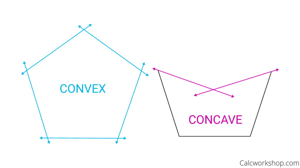
Fig.1: Some visualization for convexity
A convex edge is a type of edge that is part of a convex surface or shape. It is an edge where the surface or shape curves outward, away from the observer, along the entire length of the edge. For example, in Fig.1, all the edges in the left polygon are convex, while the interior edges with pink coloring on the right polygon are not.
A concave shape is characterized by at least one region or part that curves inward, creating an indentation or hollow area. It has sections that are “caved in” or indented. They can have complex curvatures and may require additional consideration in calculations and analysis.
Understanding the difference between convex and concave shapes is important in geometry and various fields such as computer graphics, physics, and design. Convex shapes are often preferred for their simplicity and ease of analysis, while concave shapes offer more intricate and varied forms that can be utilized creatively.
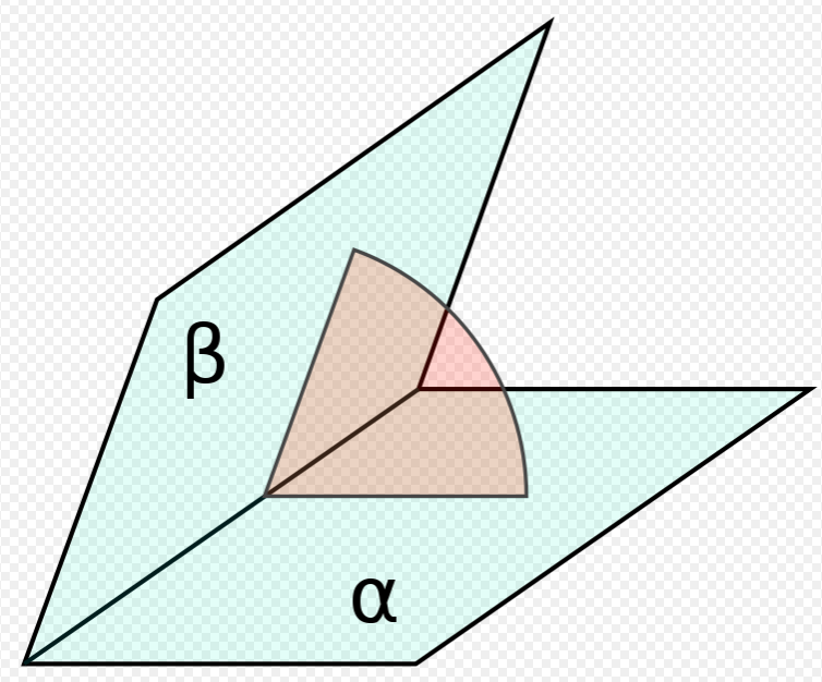
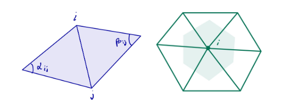
Fig.2: Dihedral angle between two half-planes (α, β, pale blue) in a third plane (red) which cuts the line of intersection at right angles
To determine which edges in the mesh exhibit concavity with dihedral angles, we followed a step-by-step process:
Compute unit normals per triangle:
Calculate the unit normal vectors for each triangle in the mesh. The unit normal represents the direction perpendicular to the surface of each triangle.
Compute the sine of the interior angles:
Since the calculated dihedral angles between two normals of triangles are treated as inner angles by our calculation. They were always between (0,180). We realized we needed a sign to differentiate between them. After searching, we found that:
A polygon with n vertices, p1,…,pn, is considered convex if, when its vertices are considered cyclically (with p1=pn), the cross products of consecutive edges,bi=(pi-pi-1) (pi+1-pi), all have the same sign or are zero. This means that the sine of the interior angles at each vertex, θi, has the same sign. If all sinθi are nonnegative or all nonpositive, the interior angles are at most 180°, indicating a convex polygon. If all sinθi are positive or all negative, the interior angles are strictly less than 180°, also indicating a convex polygon. This method allows determining polygon convexity without needing to check every angle explicitly, exploiting the properties of the sine changing sign for angles less than zero or greater than 180°.
In a formulated way, if na and nb are the normals of the two adjacent faces, and pa and pb vertices of the two faces that are not connected to the edge, wherein na and pa belong to the face A, and nb and pb to the face B, then
3. Compute the dihedral angle between two triangles:
Determine the angle between the unit normals of two triangles that share an edge. This angle represents the deviation between the neighboring triangles indicates concavity degree. When the angle is close to 180 degree, we behave this edge as convex.
By following these steps and applying them to the given mesh, we were able to identify the concave edges. The result is a set of edges that exhibit concavity, which can be further analyzed or utilized for the intended purpose.
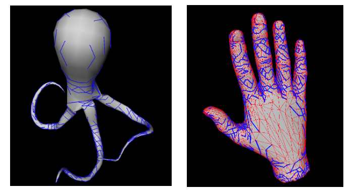
Here are some visualizations: For visualization, we have utilized Coin3D which is an OpenGL-based, 3D graphics library.
Fig.3: Our result with detected concave edges (marked with blue). For the hand model on the right, the red edges are convex edges whereas blue edges are concave.
The OFF files are from the following: Xiaobai Chen, Aleksey Golovinskiy, and Thomas Funkhouser, (A Benchmark for 3D Mesh Segmentation)[https://segeval.cs.princeton.edu/public/paper.pdf] ACM Transactions on Graphics (Proc. SIGGRAPH), 28(3), 2009. [(BibTex)[https://segeval.cs.princeton.edu/public/bibtex.html]]
2.1.2. Concavity Measurement in 3D Meshes using Qhull
This method involves collecting triangles that share specific edges, creating a point set from these triangles, and then calculating the difference between the point set and its convex hull. Through this exploration, we sought to understand the significance and applications of this novel concavity measure using Qhull for analyzing 3D meshes.
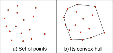
Fig.4: Example of a convex hull for a given point set
The Significance of the New Concavity Measure: The new concavity measure provides a more holistic understanding of the concavity distribution throughout a 3D mesh. By identifying regions of concavity and analyzing the curvature around specific edges, this method offers valuable insights into the overall shape and structure of complex 3D geometries.
Our Understanding of the Convex Hull Algorithm: Before delving into the implementation of the new concavity measure, it is essential to grasp the concept of the convex hull algorithm.
The convex hull represents the smallest convex shape that encloses a set of points in 2D (a polygon) or 3D (a polyhedron). The widely used Quickhull algorithm follows steps such as finding extreme points, dividing and conquering, recursion, and merging to compute the convex hull efficiently.
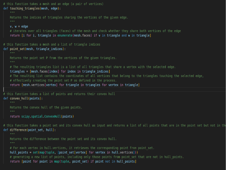
What We Have Done: To calculate the new concavity measure for a given edge (v-w), the process involves the following steps:
a. Identifying touching triangles: Iterate through the mesh to find all triangles sharing the vertices v and w, defining the selected edge.
b. Creating a point set (P): Extract all vertices from the touching triangles and collect them into a single set, forming point set P. Each vertex represents a point in 3D space and contributes to the overall shape of the region around the selected edge.
c. Computing the convex hull: Utilize the convex hull algorithm, such as the Quickhull algorithm, to determine the convex hull of point set P. The convex hull forms a closed shape that encloses all points in the point set.
d. Calculating the difference: Subtract the vertices of the convex hull from point set P to obtain the regions of concavity. These points represent areas where the mesh deviates inward and create indentations or concavities rather than forming part of the convex hull’s outer boundary.
Fig.5: Our code block in python for the specified steps (a-d)
Repeating the Process for Other Edges: To explore concavity across different parts of the mesh, the entire process can be repeated for other edges. By selecting a new edge (v’-w’) and following the steps of creating a point set, computing the convex hull, and calculating the difference, we can gain unique insights into the concavity distribution and shape features across various regions of the 3D mesh.
Visualization and Interpretation: Visualizing the results of the new concavity measure allows for a more intuitive understanding of the regions exhibiting pronounced concavities. By analyzing the difference between the point set P and its convex hull, researchers and designers can identify critical areas with concavities, evaluate surface quality, and optimize the mesh shape if needed.
2.2 Insights into Mesh Decomposition
There are various algorithms and methods for performing 3D convex decomposition, and the complexity of these methods can vary depending on the input object’s complexity and the desired level of accuracy in the decomposition.
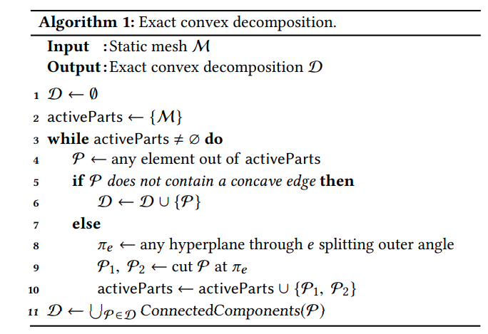
We worked on the idea based on the algorithm (Fig.6) by Approximate Convex Decomposition paper (Thul, D. et al. (2018) Approximate convex decomposition and transfer for animated meshes, ACM Transactions on Graphics. Available at: https://dl.acm.org/doi/10.1145/3272127.3275029.).
Dividing the mesh through concave edges gives the exact solution but it is intractable; so as an approximation we decided to go with Breadth-First-Search (BFS) starting from each vertex. Then grow as long as no concave edge is visited. At the end, we tried to keep the maximum connected component guided by the two measures mentioned above.
Fig.6: The exact mesh decomposition algorithm-Thul, D. et al. (2018)
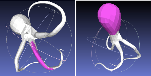
Fig.7: Highlighted regions identified as convex in 2.3. Visualized in MeshLab
2.3 An alternative approach:
A separate angle worked using a half-edge data structure to traverse the mesh. An existing half-edge data structure was heavily modified to suit the purposes of this project. The goal was to identify regions of faces connected only by convex edges using a breadth-first search, and then find the largest convex region. Early attempts resulted in non-planar regions, so the next iteration of the algorithm tracked the number of faces, edges and vertices and used the Euler formula for planar graphs to force the region of faces to remain a planar graph.
The final iteration was to apply a rule that checked that new triangles were not outside the existing region (as determined by planes formed by triangles with a concave edge), while allowing for slightly concave edges, in addition to earlier rules. This process was similar to the process for exact 3D decomposition, except that the algorithm does not check whether existing triangles should be eliminated by new concave edges. Using this method resulted in slightly more reasonable shapes for the 5 largest “convex” regions on the squid (one such region is highlighted in the Fig. 7).
3. Conclusion:
Because of our time limit, we have looked at specific parts of decomposition techniques.
Here is our comparison for these two concavity measures: Computing dihedral angles is a simple and efficient method for detecting concave edges and can be combined with BFS search method to retrieve convex components.
On the other hand, the concavity measure using Qhull offers a powerful approach to analyzing 3D meshes and understanding concavity distribution in complex geometries. By identifying regions of concavity and analyzing curvature around specific edges, this method provides valuable insights for various applications in computer graphics, computational geometry, and engineering. The ability to repeat the process for different edges allows for a detailed exploration of concavity throughout the entire 3D mesh, leading to improved surface quality assessment and shape optimization. Embracing this new concavity measure will undoubtedly enhance our understanding of complex 3D geometries and contribute to advancements in computer graphics and design.
Students: Gabriele Dominici, Daniel Perazzo, Munshi Sanowar Raihan, Biruk Abere, Sana Arastehfar
TA: Jiri Mirnacik
Mentor: Tongzhou Wang
Introduction
In reinforcement learning (RL), an agent is placed in an environment, and is required to complete some task from a starting state. Traditionally, RL is often studied under the single-task setting, where the agent is taught to do one task and one task only. However, multi-task agents are much more general and useful. A robot that knows to do all household tasks is much more valuable than one that only opens the door. In particular, many useful tasks of interest are goal-reaching tasks, i.e., reaching a specific given goal state from any starting state.
Each RL environment implicitly defines a distance-like geometry on its states:
“distance”(state A, state B) := #steps needed for an agent to go from state A to state B.
Such a distance-like object is called a quasimetric. It is a relaxation of the metric/distance function in that it can be asymmetrical (i.e., d(x,y) != d(y,x) in general). For example,
Going up a hill is harder than going down the hill.
Dynamic systems that model velocity are generally asymmetrical (irreversible).
Asymmetrical & irreversible dynamics occur frequently in games, e.g., this ice-sliding puzzle. (Game: Professor Layton and Pandora’s Diabolical Box)
This quasimetric function captures how the environment evolves with respect to agent behavior. In fact, for any environment, its quasimetric is exactly what is needed to efficiently solve all goal-reaching tasks.
Quasimetric RL (QRL) is a goal-reaching RL method via learning this quasimetric function. By training on local transitions (state, action, next state), QRL learns to embed states into a latent representation space, where the latent quasimetric distance coincides with the quasimetric geometry for the environment. See https://www.tongzhouwang.info/quasimetric_rl/ for details.
The QRL paper explores the control capabilities of the learned quasimetric function, but not the representation learning aspects. In this project, we aim to probe the properties of learned latent spaces, which have a quasimetric geometry that is trained to model the environment geometry.
Setup. We design grid-world-like environments, and use an provided implementation of QRL in PyTorch to train QRL quasimetric functions. Afterwards, we perform qualitative and visual analyses on the learned latent space.
Environments
Gridworld with directions
In reinforcement learning for the Markov decision process, the agent has access to the internal state of the world. When the agent takes an action, the environment changes accordingly and returns the new state. In our case, we try to simulate a robot trying to reach a goal.
Our agent has only three actions: go forward, turn right and turn left. We assume that the agent has reached the goal if it is around the goal with a small margin of error. For simplicity, we fix the initial position and the goal position. We set the angular velocity and the step size to be fixed for the robot.
The environment returns to the agent the position it is currently in, and the vector direction the robot is currently facing. Following the example in the original QRL paper, we have a constant reward of -1 for the agent which encourages the agent to reach the goal as quickly as possible.
Training
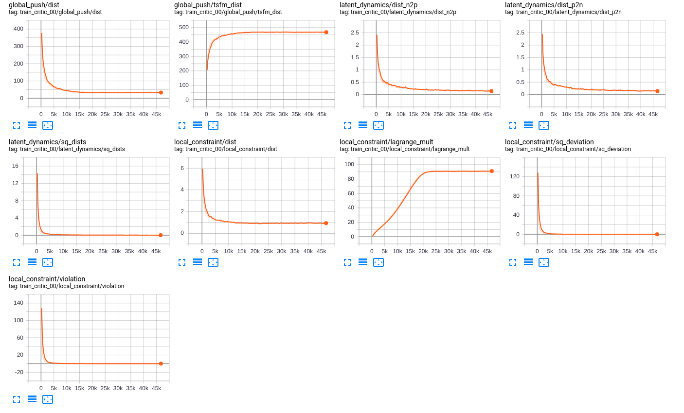
For this project, we tested QRL on the aforementioned environments, where we obtained some interesting results. Firstly, we performed an offline version of QRL using only a critic network. For this setting, we used a dataset of trajectories created by actors performing a random trajectory. This random trajectory is then loaded when training starts.As shown in the figure in the previous section, we have a robot performing a random trajectory.
We trained in QRL varying the parameters for training the neural network. Using QRL we let the network train for various steps, as can be seen below:
After performing this training we analysed what would the agent learn, however, unfortunately, it seems that the agent is stuck, as can be seen in the figure below:
To get a better understanding of the problem, we performed some experiments using A2C implementation from stable_baselines. Instead of using the angle set-up as mentioned early, we used a setting where we return the angle directly. We also performed various runs, ~10 for A2C and always testing the trajectories. Although there were some runs that A2C did not manage to find the right trajectory, on some it did. We show the best results bellow:
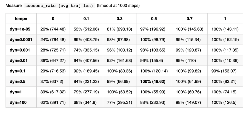
We also performed some tests varying the parameters for quasimetric learning and inserting an intermediary state for the agent to reach the goal. After varying some parameters, including batch size and the coordinate space the agent is traversing. The improved results can be seen bellow, where the agents manage to reach the goal. Also, instead of, during the visualization, instead of using a greedy approach we instead use a categorical distribution, varying a temperature parameter to make it more random:
These results were preliminary and we will not analyze these results for the next section.
We also performed an analysis on different settings, using different weights for our dynamic loss and and varying the previously mentioned temperature parameter. The table is shown bellow
Analyses
As previously said, we inspect the latent space learnt by the neural network to represent each state. In such a manner, it would be possible to inspect how the model reasons about the environment and the task.
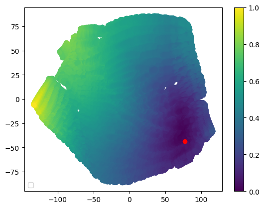
To do so, we sampled via a grid of parameters the state space of the Gridworld with directions environment. The grid was computed across 50 x values, 50 y values and 16 angle values equally separated. Then, we stored the latent representation computed by the model for each state and applied a t-SNE dimensionality reduction to qualitative evaluate the latent space referred to the state space.
Figure 6: t-SNE representation of the latent space of the state space. The color represents the normalized predicted quasimetric distance between that state and the goal (red dot).
Figure 6 shows how these latent spaces learned by the model are meaningful with respect to the predicted quasimetric distance between two states. Inspecting it more in depth, it is possible to see how it also has some properties in this environment. Mostly, if you move along the x-axis in the reduced space, you advance in the y-axis in the env with different angles, while if you move along the y-axis in the reduced space, you advance in the x-axis in the environment. In addition, we believe that this behavior would also be present in other environments, but it needs further analysis.
We also inspect the latent space learnt at different levels of the network (e.g. after including the possible actions and after the encoder in the quasimetric network), and all of them have similar representations.
Conclusion & Future directions
Even in basic environments with limited action spaces, understanding the decision-making of agents with policies learned by neural networks can be challenging. Visualization and analysis of the learned latent space provide useful insights, but they require careful interpretation as results can be misleading.
As quasimetric learning is a nuanced topic, many problems from this week remain open and there are several interesting directions to pursue after these initial experiments:
Investigate the performance of quasimetric learning in various environments. What general properties of the environment are favorable for this approach?
Analyze world-models and multi-step planning. In this project, we examined only a 1-step greedy strategy.
Formulate and analyze quasimetric learning within a multi-environment context.
Design and evaluate more intricate environments suitable for real robot control
This is a follow up to a previous blogpost. We recommend that you read the previous post before this one.
We devoted our second week to exploring three methods of ensuring temporal consistency between runs of the Latent-NeRF code:
1. fine-tuning
2. retraining a model halfway through
3. deforming Latent-NeRFs with NeRF-Editing.
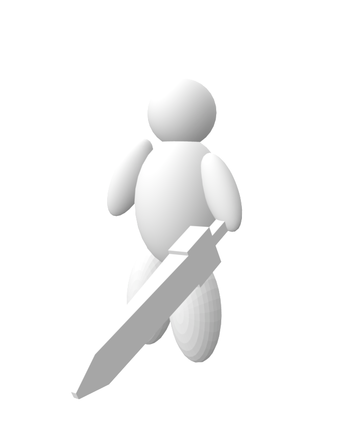
The overall aim was to keep certain characteristics of the generated images, for example, of a Lego man, consistent between runs of the code. If the following tests were run:
Lego man
Lego man holding a sword
we would want the Lego man to retain his original colors, hair, and features except for his originally raised hand which we would want to now be lowered slightly and holding a sword. If we tested for a color change, for example, such as
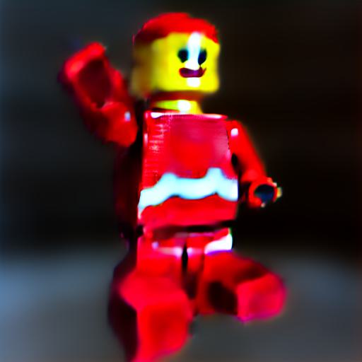
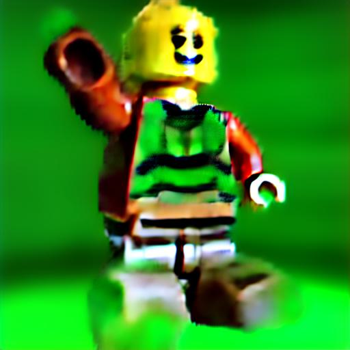
red Lego man
green Lego man
we would want the Lego man to retain exactly the same geometry between runs, with only the color of the Lego man changing as noted by the change in text guidance. After discussing ways in which to go about achieving this temporal consistency, we each decided to explore a different method, as outlined below.
1. Fine-tuning
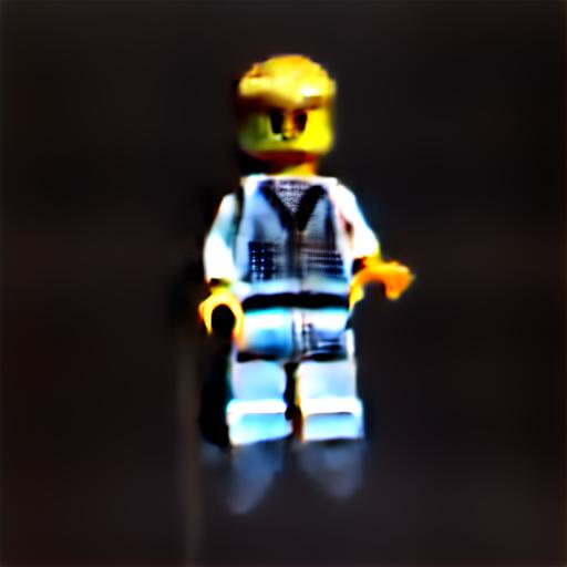
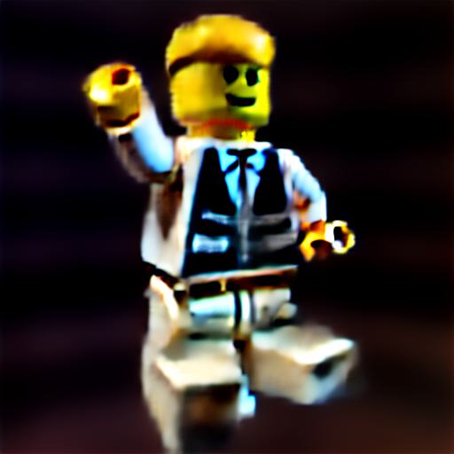
Experimental Setup The experiments were conducted using the same sketch and text prompt as a basis for animation generation. Different variations of the text prompts and sketch guides were used to observe the changes in the generated animations. The generated animations were evaluated based on color consistency, configuration accuracy, and adherence to the provided prompts. Consistency Analysis The initial experiments revealed that the model demonstrated remarkable consistency when animating a Lego man holding a sword (Figure 1). Even when the text prompt was altered to depict a teddy holding a sword (Figure 2), the generated animations still maintained accurate depictions, both in color and shape, demonstrating the model’s robustness.
Figure 1: Latent NeRF with sketch guide + text guide “a lego man holding a sword”
Figure 2: Latent NeRF output with a sketch guide and text prompt “a teddy bear holding a sword”.
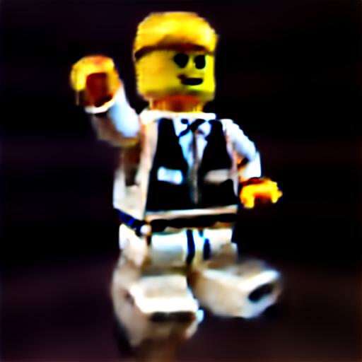
Influence of Text Prompt and Sketch Guide Figure 3 presented two different results when using the same shape guidance but different text prompts: “a Lego man” and “a Lego man with left arm up.” This indicated that the text prompt had a more significant impact on the final animation results than the sketch guide.
Figure 3: latent NeRF outputs using the same sketch guide, different text prompts. “a lego man” (left), and “a lego man with left arm up” (right), demonstrating the weight of text guide in latent NeRF.
Animation Sequence and Consistency To investigate the model’s ability to maintain consistency in an animation sequence, a series of runs were conducted where a Lego man attempted to raise the sword. After four runs, the sword’s color became inconsistent, and after the fifth run, the sword was no longer present (Figure 4).
Figure 4: Prompt: “lego man holding a sword” with different sketch shapes. The 10 sketch shapes for man animation of a humanoid figure holding a sword and raising their arm.
Fine-Tuning Techniques Three fine-tuning techniques were attempted to enhance the model’s performance on the same sketch shape guide and text prompt:
a. Full-Level Fine-Tuning Full-level fine-tuning is a technique used in transfer learning, where an entire pre-trained model is fine-tuned on a new task or dataset. This process involves updating the weights of all layers in the model, including both lower-level and higher-level layers. Full-level fine-tuning is typically chosen when the new task significantly differs from the original task for which the model was pre-trained. In the context of generating animations of a Lego man holding a sword, full-level fine-tuning was employed by using the weights obtained from a run where the generated animations had a completely visible sword. These weights were then utilized to fine-tune the model on runs where the generated animations had no swords. The outcome of this fine-tuning process showed a visible sword in the generated animations, but the boundary for the configuration of the Lego man appeared less-defined as observed in Figure 5. This suggests that while the model successfully retained the ability to depict the sword, some aspects of the Lego man’s configuration might have been compromised during the fine-tuning process. Fine-tuning at the full level can be advantageous when dealing with highly dissimilar tasks, but it also requires careful consideration of potential trade-offs in preserving specific features while adapting to the new task.
Figure 5: The output of sketch guided and text guided “a lego man holding a sword”, where the sword was no longer visible (left) and full level fine tuning output (right).
b. Less Noise Fine-Tuning We performed fine-tuning on the stable diffusion model by increasing the number of training steps. The idea behind this was to take advantage of increased interactions between the model and the input data during training, as larger time steps can provide a better understanding of complex patterns. Surprisingly, this approach resulted in a decline in both configuration and color consistency in the generated animations, as evidenced in Figure 6.
Figure 6: The output of Latent-NeRF after altering the training steps from 1000 to 2000 in the stable diffusion.
In an effort to improve the model’s performance, we experimented with adjusting the noise level in the generated data. Originally, the noise level gradually decreased from the start to the end of training. However, we decided to explore an alternative approach using the squared cosine as a beta scheduler to stabilize training and potentially enhance the quality of generated samples. Unfortunately, this adjustment led to even further degradation in both configuration and color consistency, as shown in Figure 7.
Figure 7: Changing the beta schedule from “scaled_linear” to “squaredcos_cap_v2” in Stable Diffusion.
These results indicate that finding an optimal balance between noise level and training steps is crucial when fine-tuning the stable diffusion model. The complex interplay between these factors can significantly impact the model’s ability to maintain configuration and color consistency. Further research and experimentation are needed to identify the most suitable combination of hyperparameters for this specific generative model.
c. Freeze Layers Freezing layers during fine-tuning is a widely used technique to retain learned representations in specific parts of the model while adapting the rest to new data or tasks. In our experiment involving the pre-trained model for “the Lego man holding a sword,” we employed this approach to leverage the visible sword results and enhance the performance on the scenario where the sword was not visible.
To achieve this, we selectively froze layers from different networks responsible for color and background. However, the outcomes were mixed. When we froze the sigma network layer, we observed a visible sword in the generated animations. However, there was a trade-off as the configuration of the Lego man suffered, and the depiction became less defined as shown in Figure 8.
Figure 8: Freezing sigma network layers, you can see the before this fine tuning (top) there are no swords, and after fine tuning (bottom) there is a phantom of the sword.
On the other hand, freezing the background layer led to a different outcome. While the Lego man’s configuration was better preserved, the generated animations lacked the complete depiction of the Lego man and appeared incomplete as depicted in Figure 11.
These results suggest that freezing specific layers can have both positive and negative impacts on the generated animations. It’s important to strike a balance when deciding which layers to freeze, as it can greatly influence the final performance of the model. Fine-tuning a generative model with frozen layers requires careful consideration of the specific characteristics of the task and the trade-offs between preserving existing knowledge and adapting to new data. Further experimentation is necessary to identify the optimal configuration for freezing layers in order to achieve the best results in future fine-tuning endeavors.
Conclusion The study explored the consistency and fine-tuning techniques of a generative model capable of animating a Lego man holding a sword. The model demonstrated high consistency when generating animations based on different prompts and sketch guides. However, fine-tuning techniques had varying effects on the model’s performance, with some approaches showing improvements in certain aspects but not others. Further research is necessary to achieve more reliable and consistent fine-tuning methods for generative animation models.
2. Can you retrain a NeRF midway through training?
The second approach was to modify text/shape guidance halfway through a training set, with the motivation of ensuring consistency of the elements not changed in the guidance. The idea between this method was to somehow “save” the initial conditions of the trained NeRF from the original text and/or geometry guidance so that the second set of text/geometry instructions would change only the minimal elements needed to align with the new guidance. To test this approach, we looked at three types of changes: 1) a change in the text guidance only, 2) a change in the geometry guidance, and 3) a change in both instructions.
Changing Text Guidance When only the text guidance was changed, as shown in the modification to the aforementioned lego_man configuration file below,
log:
  exp_name: 'lego_man'
guide:
  text: 'a red lego man'
  text2: 'a green lego man'
  shape_path: shapes/teddy.obj
optim:
  iters: 10,000
  seed: 10
render:
  nerf_type: 'latent'
the NeRF was able to retrain to the new text guidance with some difficulty. The results below show a snapshot of the final result of the text guidance “a red lego man” and “a green lego man”, as well as the final 3D video of the green lego man. They show how although there are still some remnants of red in the green lego man and the design of his outfit had slightly changes, the basic geometry of the lego man as well as the design in white on the red lego man and then in black on the green lego man is unchanged:
Changing Geometry Guidance When only the geometry guidance was changed, as shown in the lego_man configuration file below,
the NeRF had more difficulties retraining to match the new geometry of the lego man holding a sword. We show the two object files below that were used for these runs.
The results below show a snapshot of the final result of using the teddy.obj file for geometry guidance and then using the raise_sword.obj file, as well as the final 3D video of the second run using the raise_sword.obj file:
Changing Both When both the text and geometry guidance were changed, as shown below,
log:
  exp_name: 'lego_man'
guide:
  text: 'a lego man'
  text2: 'a lego man holding a sword'
  shape_path: shapes/teddy.obj
  shape_path2: shape/raise_sword.obj
optim:
  iters: 10,000
  seed: 10
render:
  nerf_type: 'latent'
the NeRF was able to retrain to the new guidance with less difficulty than in the case of the only using geometry guidance, yet the sword itself is somewhat translucent, and the outfit of the lego man changed from the original tuxedo look of the first run:
In conclusion, although these runs show promise for this approach of retraining a NeRF halfway through, they also indicate that there are certain initial conditions that either change completely in the retraining of the NeRF, or that inhibit the NeRF from being able to generate an accurate retrained 3D figure that corresponds to the new text and/or geometry guidance. Additionally, training data indicates that the learning curve for NeRFs may complicate the approach of retraining, as the NeRF learns certain final details only at the very end of training.
3. Deforming Latent-NeRFs with NeRF-Editing
Background Since NeRFs are functions that provide the color and volume density of a scene at a given 3D point, they do not directly generate images. Instead, a NeRF needs to be rendered just like a triangle mesh or other 3D representation would. This is done using a volumetric rendering algorithm. For each pixel in the image, a ray is shot from the camera. The color and volume density is sampled along the ray the pixel’s color is computed from those values.
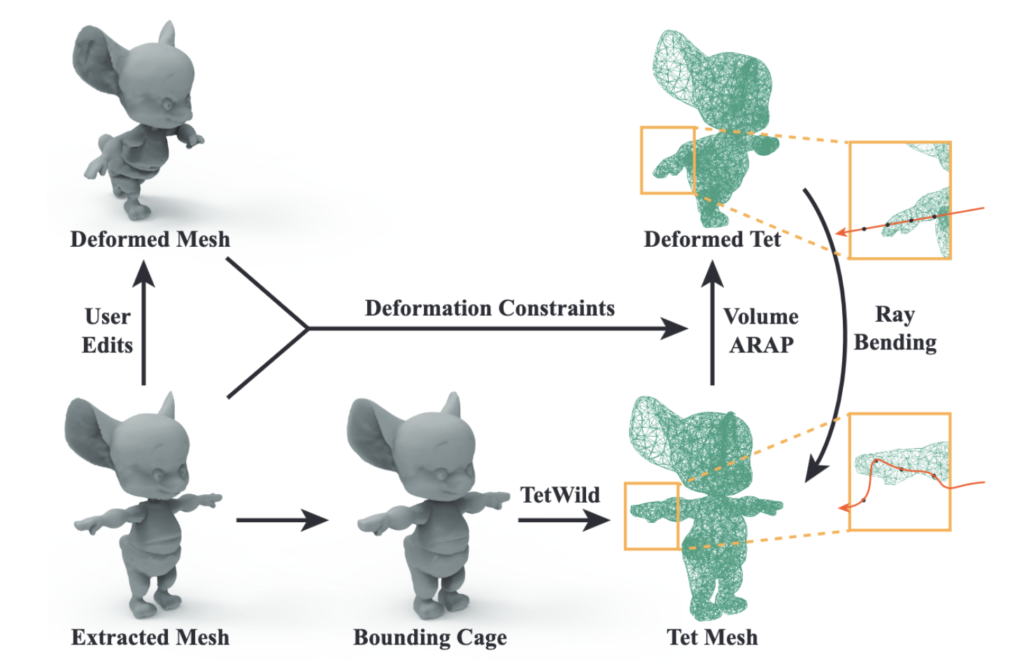
Nerf-Editing is a method that can be used to deform NeRFs. It extracts a triangle mesh from the surface of the NERF which the user can edit using whatever tools they desire. The original triangle mesh is then used to create a corresponding tetrahedral mesh. Then, the deformation of the triangle mesh is transferred to the tetrahedral mesh. This results in an original and deformed tetrahedral mesh. When the NeRF is rendered, rays are shot into the scene and points on the deformed tetrahedral mesh are sampled. Instead of sampling the NeRF at that point, the NeRF is sampled at the corresponding point on the undeformed mesh. This gives the NeRF the appearance of deformation when it is rendered to an image.
Figure: An overview of NeRF-Editing.
Proposed Process Latent-NeRF can be guided with a sketch-shape. Ideally a user would able to deform the sketch shape and get a deformed NeRF back. We start with a sketch-shape and train a corresponding Latent-NeRF. We then put the trained NeRF into NeRF-Editing. Instead of extracting a triangle mesh to get an editable representation of the NeRF, we simply use the sketch-shape. The user edits the sketch-shape. We tetrahedralize the original sketch-shape and create a corresponding deformed tetrahedral shape. We then render the NeRF by sampling points on the deformed shape and then sampling the NeRF in the corresponding un-deformed location. It would be interesting to see whether the sketch shape would be enough to guide the deformation instead of a mesh extracted from the NeRF itself.
Challenges The main challenge is that there are many different NeRF architectures since there are many ways to formulate a function from points in space and view direction to color and volume density. Latent-NeRF uses an architecture called Instant-NGP which stores visual features in a data structure called a hash grid and uses a small neural network to decode those features into color and volume density. NeRF-Editing uses a backend called NeuS. NeuS is an extension on the original NeRF method, which utilized one massive neural network, and embedded a signed distance function better define the boundaries of shapes. In theory, NeRF-Editing’s method is architecture agnostic, but the implementation of Instant-NGP into NeRF-Editing was too time consuming for the 2-week project timeline.
Students: Tewodros (Teddy) Tassew, João Pedro Vasconcelos Teixeira, Shanthika Naik, and Sanjana Adapala
TAs: Andrew Rodriguez
Mentor: Karthik Gopinath
1. Introduction
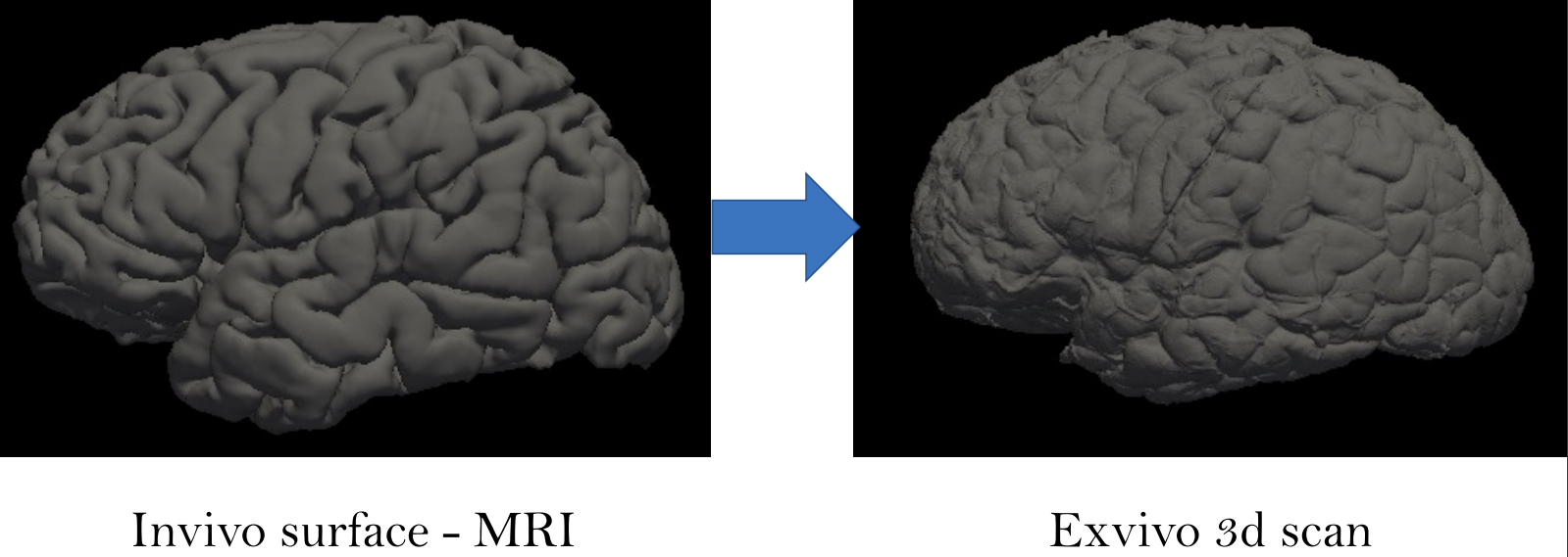
Ex-vivo surface mesh reconstruction from in-vivo FreeSurfer meshes is a process used to construct 3D models of neurological structures. This entails translating in-vivo MRI FreeSurfer meshes into higher-quality ex-vivo meshes. To accomplish this, the brain is first removed from the skull and placed in a solution to prevent deformation. A high-resolution MRI scanner produces a detailed 3D model of the brain’s surface. The in-vivo FreeSurfer mesh and the ex-vivo model are integrated for analysis and visualization, making this process beneficial for exploring brain structures, thereby helping scientists learn how it functions.
Figure 1 Converting in-vivo surface to exvivo 3d scan
2. Approach
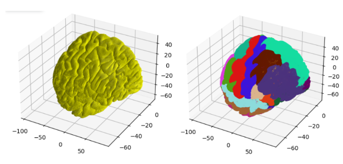
This project aims to construct anatomically accurate ex-vivo surface models of the brain from in-vivo FreeSurfer meshes. The source code for our project can be found in this GitHub repo. A software tool called FreeSurfer can be used to produce cortical surface representations from structural MRI data. However, because of distortion and shrinking, these meshes do not adequately depict the exact shape of the brain once it is removed from the skull. As a result, we propose a method for producing more realistic ex-vivo meshes for anatomical investigations and comparisons. For this task, we used five in-vivo meshes which were provided along with their annotations. Figure 2 shows a sample in-vivo mesh and its annotation.
Figure 2 Sample in-vivo mesh and its annotation
We attempted to solve this using two different spaces:
Volumetric space
Surface space
2.1. Volumetric Space
Our volumetric method consists of the following steps:
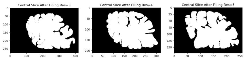
First, we fill in the high-resolution mesh into a 3D volume. This process ensures that the fine details of the cortical surface, such as gyri and sulci, are preserved while avoiding holes or gaps in the mesh. We performed the filling operation at three different resolutions which are 3,4 and 5 using FreeSurfer’s “mris_fill” command.
Figure 3 Central slice for different resolutions after filling
The deep sulci of the brain are then closed. Sulci are the grooves or fissures in the brain that separate the gyri or ridges. These sulci can sometimes be overly deep or too wide, affecting the quality of brain imaging or analysis. This step is necessary because in-vivo meshes often include open sulci which are not visible in the ex-vivo condition due to tissue collapse and folding. By closing the sulci, we can obtain a smoother and more compact mesh that resembles the ex-vivo brain surface.
Figure 4 Central slice for different resolutions after closing
Morphological operations are methods that change the shape or structure of a shape depending on a preset kernel or structuring element. There are a number of morphological operations, but we will concentrate on three here: dilation, fill and erode. Dilation extends an object’s borders by adding pixels to its edges. Fill adds pixels to the interior of an object to fill in any holes or gaps. Erode reduces the size of an object’s bounds by eliminating pixels from its edges. We can apply morphological operations to smooth out the brain surface and close the gaps to remedy this problem.
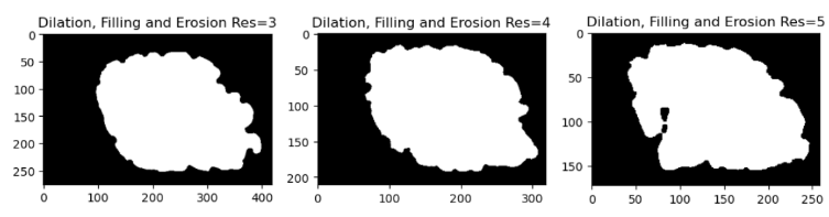
We used the following operations in a specified order to close the deep sulci of the brain: dilation, fill and erode. We first dilate the brain image to make the sulci smaller and less deep. The remaining spaces in the sulci are then filled to make them disappear. Finally, the brain image is eroded to recover its original size and shape. As a result, the brain surface is smoother and more uniform, with no deep sulci.
Figure 5 Central slice for different resolutions after dilation, filling, and erosion
The extraction of iso-surfaces from the three-dimensional volumetric data is accomplished using the well-known algorithm Marching Cubes, which results in a more uniform and accurate representation of the brain surface. This process transforms the three-dimensional volume into a surface mesh that can be visualized and examined.
Then we used the Gaussian smoothing algorithm in order to smooth the output of the marching cubes algorithm. In order to smooth an image, a Gaussian function is applied to each pixel using a Gaussian blur filter. Often employed in statistics, the normal distribution is mathematically described by a function called a Gaussian function. A Gaussian function in one dimension has the following form:
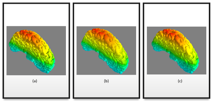
Figure 4 shows the visualization results of the reconstruction results before and after the application of Gaussian smoothing.
Figure 7 (a) original mesh, (b) reconstructed mesh using marching cubes without smoothing, (c) reconstructed mesh after smoothing.
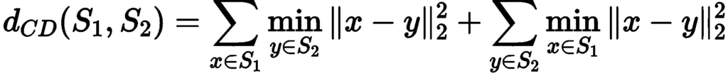
Finally, we used the density-aware chamfer distance to assess the quality of the reconstructed mesh. For comparing point sets, two popular metrics known as Chamfer Distance (CD) and Earth Mover’s Distance (EMD) are commonly used. While EMD focuses on global distribution and disregards fine-grained structures, CD does not take into account local density variations, potentially disregarding the underlying similarity between point sets with various density and structure features. We define the chamfer distance between two pointsets using the formula below:
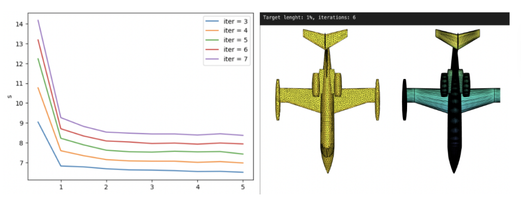
From the reconstruction results, we can visually see that when the resolution increases the result is not so great. After performing the morphological operations we can see that the results for resolution of 5 still have some holes and the sulci is still deep. While for the lowest resolution of 3, we can see that the reconstruction is closer to ex-vivo than in-vivo. In order to validate our assumptions from the visualization, we computed the chamfer distance between the original mesh and the reconstructed mesh after the morphological operations are performed. The results after the calculation are summarized in Table 1.
Resolutions
N=10
N=100
N=1000
N=10000
3
4.15
7.62
76.26
274.73
4
5.66
10.09
42.92
182.66
5
4.53
8.60
33.19
168.83
Table 1 Chamfer distance for different resolutions
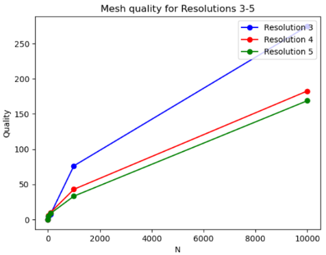
After getting the point clouds from both meshes, we only considered a subset of the vertices to compute the distance since considering the entire point cloud is computationally intensive and very slow. We took the number of vertices to be powers of 10. Then the point clouds were rescaled and normalized to be in the same space. From the results, we can conclude that the higher resolution has the lowest distance, while the lowest resolution has the highest distance. This is true from our observation that the highest resolution should be closer to the original mesh while the lowest resolution is further from it since it’s getting similar to an ex-vivo mesh. Figure 8 shows a plot of the mesh quality for the different resolutions, where the number of vertices is given on the x-axis and the distance is given on the y-axis.
Figure 8 Mesh quality for different resolutions
2.2. Surface-based approach
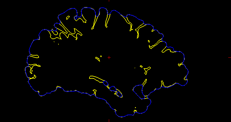
Sellán et al. demonstrate in “Opening and Closing Surfaces (2020)” that many regions don’t move when performing closing operations, and the output is curvature bound, as shown in Figure 9.
Figure 9 (yellow) Original outline, (blue) Closed outline
Therefore, Sellán et al. propose a bounded curvature-based flow for 3D surfaces that moves not curvature bound points in the normal direction by an amount proportional to their curvature.
As an alternative to the volumetric closing of the deep sulci of the brain, we applied the Sellán et al. method to close our surfaces. Figures 10 and 11 present the progressive closing of the mesh at each iteration until it converges.
Figure 10 Surface at each iteration of the closing flow
Figure 11 Outlining the difference at iterations 2, 4 and 6
2.3. Extracting External Surface
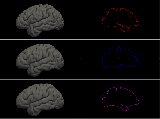
One other approach we tried to explore was focused on getting only the outer surface without all the grooves by post-processing the meshes reconstructed from the in-vivo reconstructed surface (Figure 12. a). So we followed the following steps:
Inflate the mesh by pushing each vertex in the direction of its normals. This results in the closing of all the grooves and only the external surface is directly visible. The inflated mesh is shown in Figure 12. b
Once we have this inflated surface, we need to retrieve only the externally visible surface. For this, we treat all the brain vertex as origins and shoot rays in the direction of vertex normals. The rays originating from vertices lying on the external surface do not hit any other surface, whereas the ones from the inside surface hit the external surface. Thus we can find and isolate the vertices lying on the surface. We reconstruct the surface using these extracted meshes using Poisson reconstruction. The reconstructed mesh is shown in Figure 12. c
Figure 12 Post-processing the meshes reconstructed from the in-vivo reconstructed surface
3. Future work
In this study, we presented a technique for reconstructing an ex-vivo mesh from an in-vivo mesh utilizing various methods. But there are still limitations and difficulties that we would like to address in our future studies. One of them is to mimic the effects of cuts and veins, which are common artifacts in histological images, on the surface of the brain. To achieve this, we intend to produce accurate displacement maps that can simulate the deformation of the brain surface as a result of these factors. Additionally, using displacement maps, we will investigate various techniques for producing random continuous curves on the 2D surface that can depict cuts and veins. Another challenge is to improve the robustness of our method to surface deformation caused by different slicing methods or imaging modalities. We also want to train deep learning networks such as GCN/DiffusionNet to segment different brain regions. We will investigate the use of chamfer distance as a loss function to measure the similarity between the predicted and ground truth segmentation masks, and to encourage smoothness and consistency of the segmentation results across different slices.
Fellows: Aditya Abhyankar, Munshi Sanowar Raihan, Shanthika Naik, Bereket Faltamo, Daniel Perazzo
Volunteer: Despoina Paschalidou
Mentor: Nicholas Sharp
I. Introduction
Triangular and tetrahedral meshes are central to geometry, we use them to represent shapes, and as bases to compute with. Many numerical algorithms only actually work well on meshes that have nicely-shaped triangles/tetrahedra, so we try very hard to generate meshes which simultaneously:
Represent the desired shape
Have nicely-shaped elements and
Perfectly interlock to cover the domain with no gaps or overlaps.
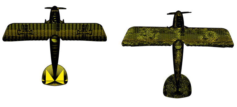
Yet, is point (3) really that important? What if instead we just sampled a soup of random nicely-shaped triangles, and didn’t worry about whether they fit together?
In this project we explore several strategies for generating such random meshes, and evaluate their effectiveness.
II. Algorithms
II.1. Triangle Sampling
Fig 1: The heat geodesic method fails if the triangles are isolated (left); but if the triangles share vertex entries, the heat method works even with gaps and intersections (right).
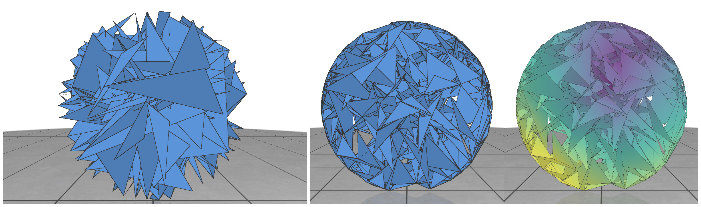
In random meshing, we are given the boundary of a shape (e.g. the polygon outline of a 2D figure) and the task is to generate random meshes to tessellate the interior. Here, we will focus mainly on the planar case, where we generate triangles with 2D vertex positions. We will test the generated meshes by running the Heat Method [2], a simulation-based algorithm for computing distance within a shape. The very first shape we tried to tessellate is a circular disk.
Since a circle is a convex shape, we can choose three random points inside the circle and any triangle is guaranteed to stay within the shape. But generating isolated triangles like these is not a good strategy, because downstream algorithms like the heat method rely on shared vertices to communicate across the mesh. Without shared vertices, it is equivalent to running the algorithm individually on a bunch of separate triangles one at a time.
Next strategy: At each vertex, consider generating n random triangles that are connected to other vertices within a certain radius. This ensures that the generated triangles share the same vertex entries. Even though these random triangles have many gaps and intersections, many algorithms are actually perfectly well-defined on such a mesh. To our surprise, the heat method was able to generate reasonable results even with these random soup of triangles (Fig 1).
II.2. Non-Convex Shapes
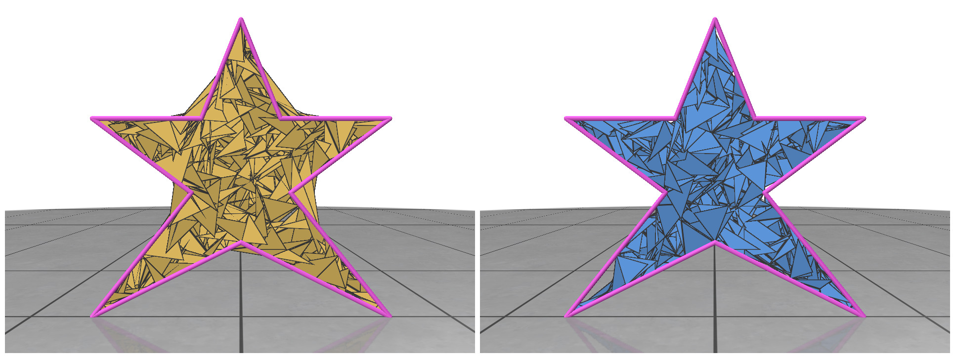
Fig 2: Random meshing of a non-convex star shape (left); mesh generated by rejection sampling of the triangles (right).
For non-convex shapes, if we try to connect any three points within the polygon, some of the triangles might fall outside of our 2D boundary. This is illustrated in Fig 2 (left). To circumvent this problem, we can do rejection sampling of the triangles. Every time we generate a new triangle, we need to test whether it is completely contained within the boundary of our polygon. If it’s not, we reject it from our face list and sample another one. After rejection, the random meshes seem to nicely follow the boundary. Rejection sampling makes our meshing algorithm a little slower, but it’s necessary to handle non-convex shapes.
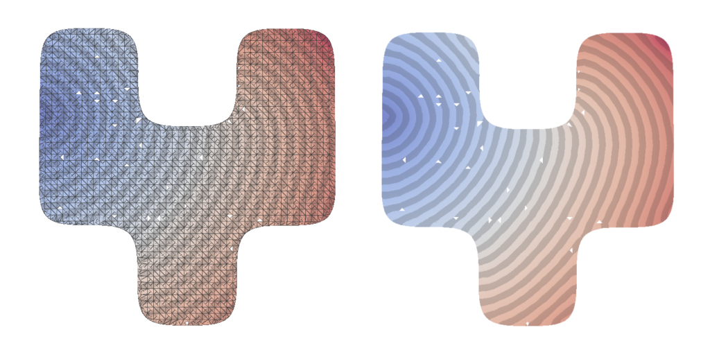
II.3. Triangle Size
Fig 3: Random meshes with different triangle size (left) and the isolines of their geodesic distance from the source (right).
In random meshes, we find that the performance of the heat geodesic method is dependent on the size of the triangles. Since we are generating triangles by sampling points within a radius, we can make the triangles smaller or larger by controlling the radius of the circle. With decreasing triangle size, the distance computed by the heat method becomes more accurate. This is illustrated in Fig 3: as the triangles become smaller, the isolines look more precise. The number of triangles are kept fixed in all cases.
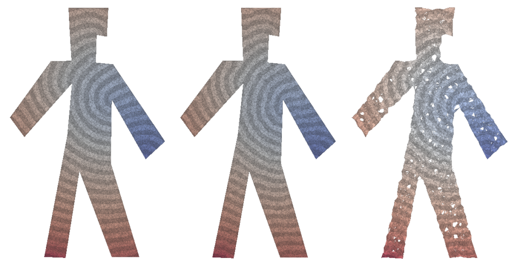
III. Visualizations and results
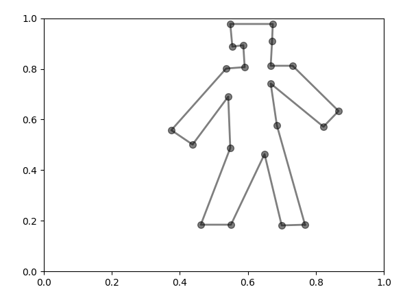
We created an interface to aid in the task of drawing different polygon shapes for visualization. As can be seen below, an example of a shape:
We can use one of our algorithms to plot various types of meshes with the distance function drawn by the heat equation. We put the visualization of these meshes bellow, where the leftmost is the mesh using Delaunay triangulation, the rightmost using random triangles and the center being using Delaunay triangulation but using the faces from the Delaunay triangulation for a better visualization.
In this case, with 5000 points sampled randomly, we have an error of 0.0002 compared with the values for the distance function compared with using the heat method.
IV. An Attempt at Random Walk Meshing
Another interesting meshing idea is spawning a single vertex somewhere in the interior of the shape, and then iteratively “growing” the mesh from there in the style of a random walk. At each iteration, every leaf vertex randomly spawns two more child vertices on the circumference of a circle surrounding it, which are used to form a new face. If any such spawning circle intersects with the boundary of the shape, we simply use the two vertices of the closest boundary edge instead to form the new face. We tried various types of random walk strategies, such as using correlated random walks with various correlation settings to mitigate clustering at the source vertex.
While this produced an interesting single component random mesh, the sparse connectivity made it a bad algorithm for the heat method, as triangle sequences that swiveled back around in the direction of the source vertex diffused heat backwards in that direction too.
This caused the distance computations to be inaccurate and rendered the other methods superior. We would like to explore this approach further though, as it might prove useful for other use-cases like physics simulations and area approximations. Random walks are very well studied in probability literature too, so deriving theoretical results for such algorithms seems like a very principled task.
V. Structure in Randomness
While sampling triangles within a radius gave a reasonable results upon calculating geodesic distance, we tried exploring ways to make it more structured. One such method we came with is grid sampling with triangulation within a neighborhood. The steps are as follows:
Uniformly sample points within a square grid enclosing the entire shape.
Eliminate points outside that fall out of the desired shape.
For each vertex within the shape, form a fan of triangles with its 1 ring neighborhood vertices.
These are the geodesic isolines on the triangular mesh obtained using the above method.
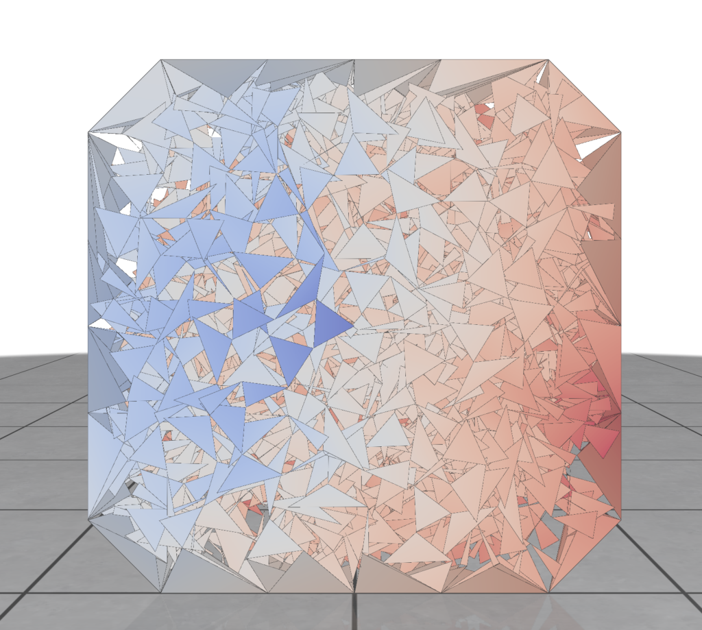
VI. Conclusion and Future Work
We present some examples of our random computation method working on 2D meshes for various different shapes. Aside from refining our algorithms and performing more experiments, one interesting avenue would be to perform experiments with tetrahedralization on 3D shapes. We have also done simple tests with current state-of-the-art tetrahedralization algorithms [3], the results are shown below. So, for future work, this would be a really interesting avenue. Another interesting avenue for theoretical work regarding random walk meshing would be computing how the density of triangles varies with iteration count and various degrees of correlation.
VII. References
[1] Shewchuk, Jonathan Richard. “Triangle: Engineering a 2D quality mesh generator and Delaunay triangulator.” Workshop on applied computational geometry. Berlin, Heidelberg: Springer Berlin Heidelberg, 1996.
[2] Crane, Keenan, Clarisse Weischedel, and Max Wardetzky. “The heat method for distance computation.” Communications of the ACM 60.11 (2017): 90-99.
[3] Hu, Yixin, et al. “Tetrahedral meshing in the wild.” ACM Trans. Graph. 37.4 (2018): 60-1.
[4] Hu, Yixin, et al. “Fast tetrahedral meshing in the wild.” ACM Transactions on Graphics (TOG) 39.4 (2020): 117-1.
Students: Francisco Unai Caja López, Shalom Abebaw Bekele and Sara Ansari Directed by Jorg Peters and Kyle Lo
1. Introduction
The goal of this project is to design a layout simplification procedure. Following [2], we define an integer-linear programming model to find a set of collapsable arcs, and merge sets of arcs to simplify the layout. The algorithm is part of a bigger research project that is currently carried out by Kyle Lo and Jorg Peters. In said project surfaces are approximated using splines and piece-wise Bezier surfaces [7].
1.1 What is a layout and why do we care about layouts?
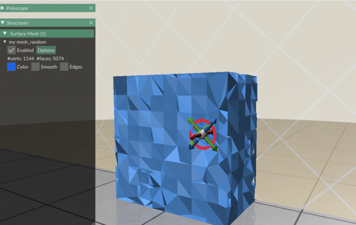
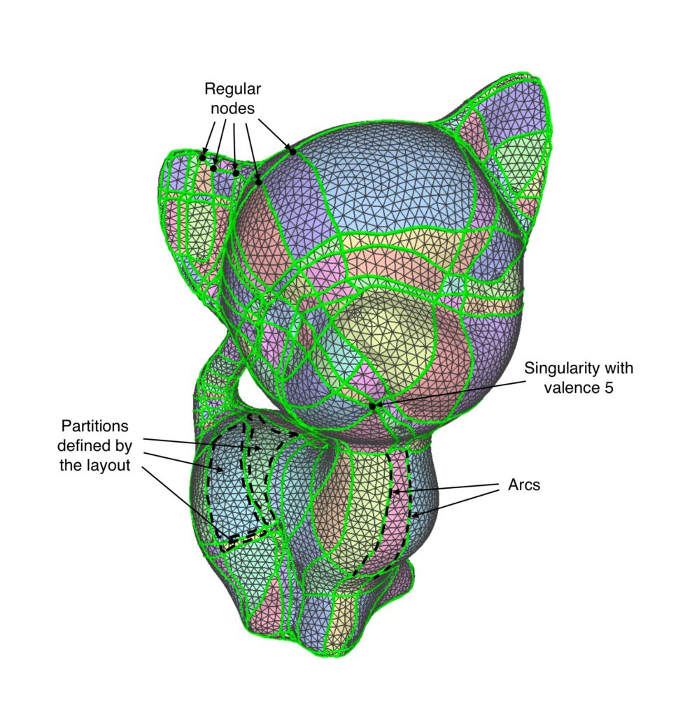
Definitions. Consider a graph M = (V,E) of a triangle mesh. For us, a layout is defined as another graph G = (N,A) where N is a subset of V called nodes and A is the set of arcs. Each arc a ∈ A is a polyline that connects two nodes via a sequence of edges from the original triangle mesh. For each node n ∈ N, we define its valence as the number of arcs incident to n. Also, a node is said to be a singularity if it has valence different than 4. Singularities are particularly important in quad layouts, that is, layouts in which all patches are 4-sided. This is because singularities usually lie near important regions and features of the surface. In the following figure you can see an example of a quad layout.
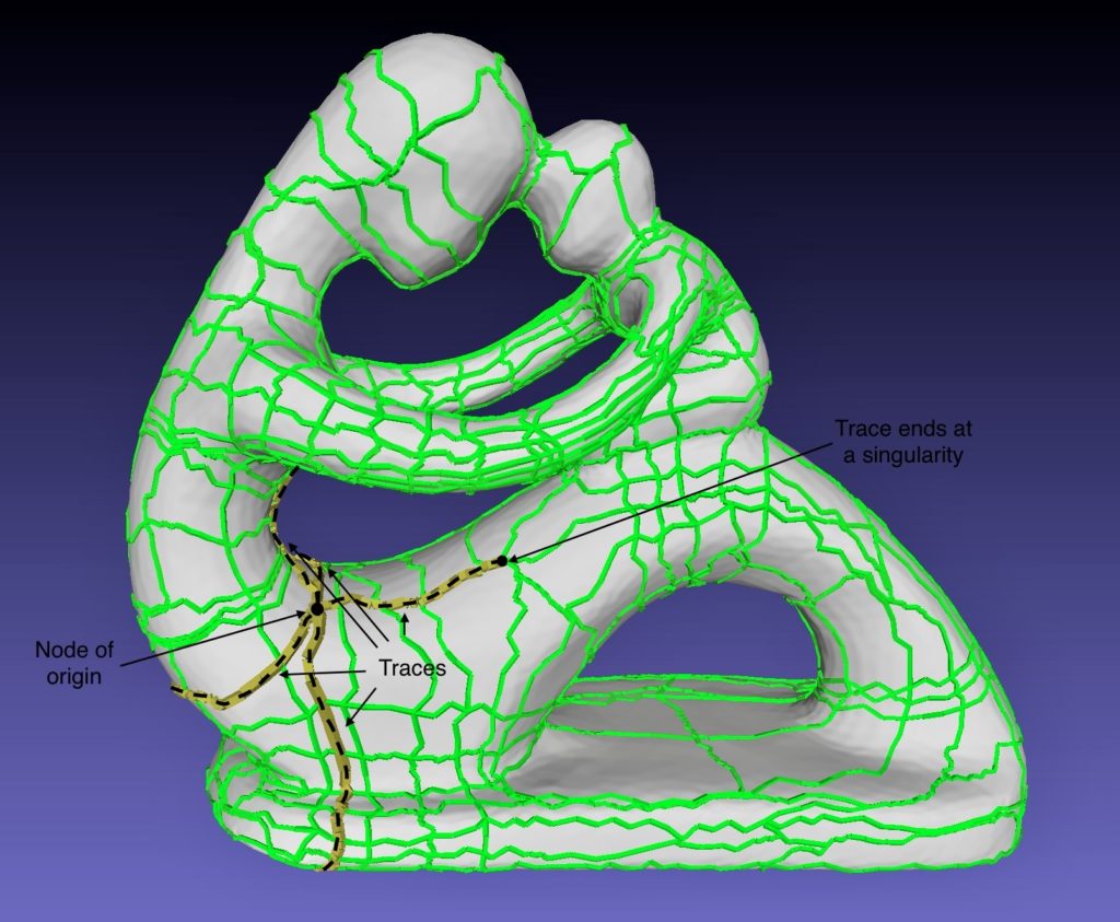
Another important concept in this project is that of a trace. Traces are polylines that begin at a singularity and travel through the layout until they reach another singularity. If we are building a trace and encounter a regular node n, the trace will continue through the opposite arc of n. The following figure shows 5 traces that originate at a particular singularity.
Layouts can describe the global structure of the mesh while also defining a partition. Moreover, layouts play a crucial role in tasks such as quadrangulation and embedding Bezier, or NURBS surfaces.
1.2 Layout generation and the objective of this project
There are various methods for generating quad mesh layouts, such as finding a set of separatrix candidates (i.e. paths connecting pairs of prescribed singularities) in topologically distinct ways, from which a subset is chosen to define a full layout [6]. Another method involves computing a cross-field from a given set of linear PDEs based on an imposed set of singularities. These singularities can occur naturally, for example, by minimizing Ginzburg-Landau energy, or as a user-defined singularity pattern [5]. The interested reader can learn more about layouts and quad meshes in [3].
In this project we are given layouts generated by a modified version of Quadwild [1]. These layouts are generated from triangle meshes. The goal is to find a subgraph of the layout with as few partitions as possible while ensuring that each pair of singularities is separated.
2. Finding collapsable arcs via integer programming
In order to simplify a layout, we first need to figure out which elements are removable. Precisely, we want to know when an arc can be collapsed. To do this, for each arc a ∈ A we define an integer variable qa. We define an integer programming model following [2]. In the paper the layouts are allowed to have T-junctions which makes it so that the variables qa can take any non negative value 0,1,2,… However, this doesn’t happen with the layouts we are working with so, just for this project, we can assume qa is binary and defined as
\(q_a = \begin{cases} 1 & \text{if arc } a \text{ is collapsable} \\ 0 & \text{otherwise} \end{cases}.\)
2.1. Constraints to enforce properties of the resulting layout
We have two main restrictions.
The resulting layout must be a quad layout
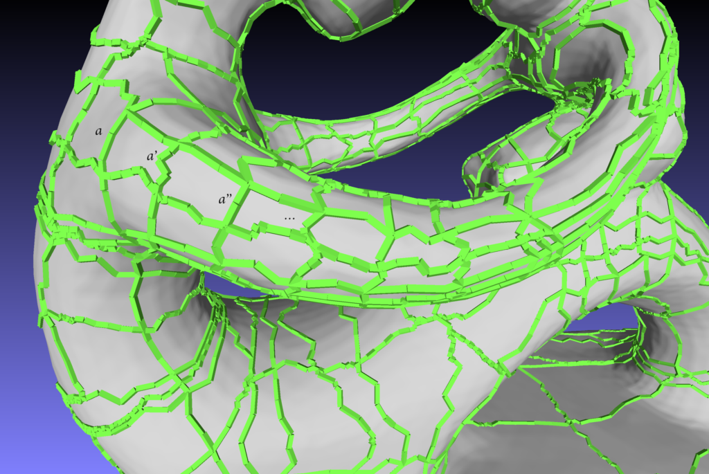
Suppose that we want to collapse arc a in the following figure, then we must also collapse all the arcs a’, a”, … Otherwise, we would have a three sided patch and the result would not be a quad layout.
More generally, if arcs a and a’ lie in the same patch and are opposite to each other, then we must have qa = qa’.
Singularities must remain separate
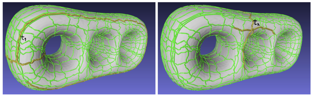
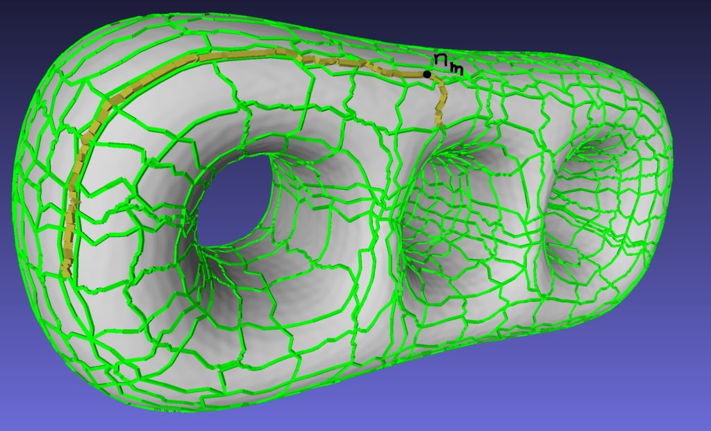
In general, singularities tend to appear near important features of the mesh or in regions with high curvature. Thus, it makes sense that we try to preserve their locations. We make sure that different singularities aren’t merged together regardless of the number of collapsed arcs. This is done by forcing that any pair of singularities are at a ”positive Manhattan distance”. More precisely, consider two singularities n1, n2 and traces t1, t2 with origin in n1 and n2 respectively. Assume that both traces go through mid node nm, then we must have
In the following figure we can see an example of a pair of intersecting traces t1 and t2.
And in the following figure we have the set of arcs that links the origin of each trace to the mid node.
One possibility to avoid collapsing two singularities together would be, for each pair of nodes n1, n2, finding intersections of all possible traces t1, t2 and add the previous restriction to the model. In that case, the number of restrictions would be quadratic in the number of nodes. However, the same result can be achieved with far fewer restrictions as is stated in [2].
Notation. For every pair of intersecting traces ti, tj, we denote the first common node as nij. The set of arcs that link the origin on ti with nij is represented by Sij and the total length of those arcs is denoted by lij. Finally, given a trace ti, we define ni* as the intersecting node which is closest to the origin of ti and verifies li* > l*i. The set of arcs that link the origin of ti with ni* will be denoted Si*.
Lemma 1 of [2] asserts that the family of restrictions
\(\sum_{a\in S_{i*}} q_a \geq 1, \quad \text{for every trace }t_i\)
implies the inequality we previously mentioned. Therefore, we can enforce the desired property using O(⎮N⎮) restrictions where ⎮N⎮ is the number of nodes.
Finally, if we just want to collapse as many arcs as possible, we could set the objective function as ∑aqa where the sum is over all arcs. This yields the following linear integer programming model
\(\begin{cases} \min & \sum_{a}q_a\\ \text{s.t.} & q_a = q_{a’} \text{ whenever } a,a’ \text{ are oposites in the same patch} \\ & \sum_{a\in S_{i*}} q_a \geq 1 \quad \text{for every trace }t_i\\ & q_a\in{0,1} \quad \text{ for every arc } a \end{cases}\)
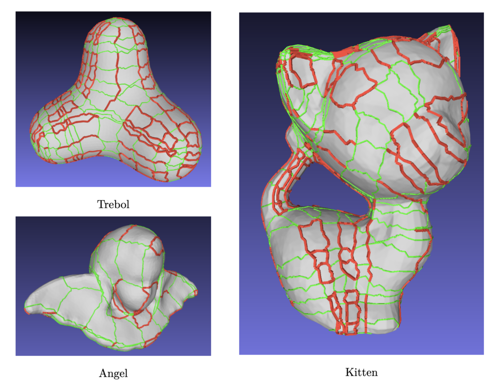
Said model will be optimized by Gurobi, a comercial solver. The output is a set of arcs that can be collapsed while maintaining the properties we desire. In the following figure we have in red the collapsable arcs according to an optimal solution to the model
We can see that many of the original arcs are collapsable.
2.2. How do we simplify a layout?
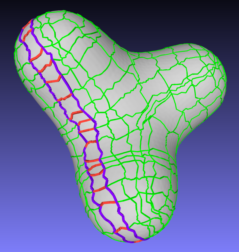
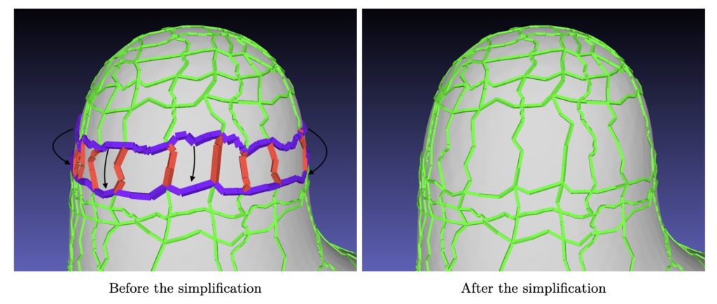
Suppose we have chosen to collapse an arc a, then we will need to collapse a whole set of arcs in order to preserve the quad structure of the layout. This collapse will be done by merging two sets of arcs together. In the following figure we see an example with the arcs to collapse in red and the arcs to merge in purple.
In this project we have chosen to ”move one of the arcs on top of the other” although there are many other choices to do this. In the following figure you can see the simplification procedure.
3. Results and future work
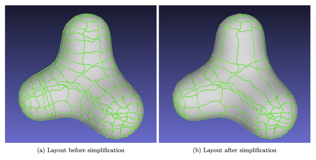
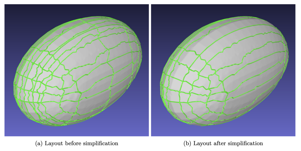
In this project we have learned about layouts and developed a procedure to simplify them iteratively. In addition, solving the integer programming problem has proved to be quite fast (under 0.05 seconds for the examples tested), as the model wasn’t too big. In the following figures you can see the result of applying the simplification several times on two different layouts.
Of course, there are a lot of aspects that can be improved and directions to continue the work
The code we developed is far from finished. For instance, we run into problems when some of the arcs to collapse are incident to singularities. All of these special cases should be considered and dealt with appropriately.
Weights could be added to variables in the objective function of the integer programming model. The objective function would look like ∑awaqa. For instance, we could define
\(\qquad \qquad \qquad \qquad \qquad \qquad \qquad \bar{k}_a = \frac{\sum{r\in R}\vert k_p^r\vert }{\vert R\vert},\quad p = \underset{i=1,2}{\text{arg max }}\vert k_i^r \cdot \vec a \vert\)
where R denotes a set of vertices close to arc a and krp is the principal curvature at vertex r that better aligns with the direction vector of the arc. Then, we could define
The motivation is that we want to preserve arcs that lie in sections with very high curvature. Having a really big patch in the layout that contains very different and intricate details is undesirable. For example, if we wanted to approximate them with splines, then we would need to use a very high degree. Such weighting scheme could be helpful to prevent the creation of such patches.
3. When merging two different arcs, we have chosen to place the new arc in the location of one of the arcs to be merged. Other strategies may be more successful, for instance, we could create a new arc that passes through a region of high curvature. This could help align arcs with features.
4. After the layout simplification, a smoothing procedure like [8] could be applied on all arcs to improve the quality of the results.
Finally, we would like to thank Justin Solomon for giving us such a wonderful opportunity by organizing SGI 2023 as well as Jorg Peters and Kyle for guiding us through this project.
[2] Lyon, M., Campen, M., & Kobbelt, L. (2021). Quad layouts via constrained t-mesh quantization. Computer Graphics Forum, 40(5), 305-314.
[3] Campen, M. (2017). Partitioning surfaces into quadrilateral patches: A survey. Computer Graphics Forum, 36(2), 567-588.
[4] Schertler, N., Panozzo, D., Gumhold, S., & Tarini, M. (2018). Generalized motorcycle graphs for imperfect quad-dominant meshes. ACM Transactions on Graphics (TOG), 37(6), 1-14.
[5] Jezdimirovic, J., Chemin, A., Reberol, M., Henrotte, F., & Remacle, J. F. (2021). Quad layouts with high valence singularities for flexible quad meshing. Retrieved from https://internationalmeshingroundtable.com/assets/papers/2021/08-Jezdemirovic.pdf
[6] Razafindtazaka, F. H., Reitebuch, U., & Polthier, K. (2015). Perfect matching quad layouts for manifold meshes. Computer Graphics Forum, 34(5), 219-228.
[7] Peters, J., Lo, K., & Karčiauskas, K. (2023). Algorithm 1032: Bi-cubic splines for polyhedral control nets. ACM Transactions on Mathematical Software (TOMS), 49(1), 1-12.
[8] Field, D. A. (1988). Laplacian smoothing and Delaunay triangulations. Communications in Applied Numerical Methods, 4(6), 709-712.
Fellows: Erik Ekgasit, Maria Stuebner, and Anna Cole
1: Introduction
Triangles are a nice way to represent the surface of a 3D shape, but they are not smooth. The tangent vectors on a triangle mesh are not continuous.
When it comes to representing curves, we can approximate a curve using a polyline, a set of points connected with straight lines. Alternatively, we could use a spline which provides a smooth way to form a curve that passes through a set of points. Splines that represent curves are piecewise polynomial functions that trace out a curve:
\(f: \mathbb{R} \rightarrow \mathbb{R}^n\).
Similarly a 3D shape’s surface can be represented using splines that are piecewise polynomial functions:
\(g: \mathbb{R}^2 \rightarrow \mathbb{R}^3\).
The Powell-Sabin construction is a type of spline whose pieces are essentially curved triangles that can represent smooth surfaces. In this project, we aim to augment the Powell-Sabin construction to accommodate sharp features on meshes.
1.2: The Powell-Sabin Construction
A triangle mesh can be fed into an optimization algorithm that constructs a spline surface that contains (or is very close to) the points occupied by vertices of the triangle mesh. The surface is also optimized to be smooth. This is done by assigning every triangle in the original mesh a Powell-Sabin patch, the parameters of which are then chosen during optimization. Additionally, the mesh must have a UV map, which assigns each point on the mesh to a point on the plane.
Suppose we have a triangle with indices \((i, j, k)\). Its corresponding Powell-Sabin patch can be specified using 12 vectors in \(\mathbb{R}^3\). Three position vectors \(p_i, p_j, p_k\) describe the positions of the vertices. During optimization, the vertices can move a small amount to create a smoother surface. Each vertex also gets two additional vectors to describe the derivative of the surface going out of each incident edge (labelled with \(d\) in the image below). Finally, each edge of the triangle has an associated vector to describe the derivative of the surface perpendicular to the edge at the midpoint (labelled with \(h\) in the image below).
1.3: Global Parameters
These parameters are not directly optimized. Instead they are derived from global degrees of freedom, which do get directly optimized. This allows more data to be shared between different triangles to ensure continuity. Each vertex in the mesh is assigned 3 vectors in \(\mathbb{R}^3\). One for position and two for a pair of tangent vectors, which are the gradients in the u and v directions in the local parametric domain chart. These gradients should be linearly independent unless the surface is somehow degenerate. Additionally, each edge gets one tangent vector. An illustration of these degrees of freedom is shown below.
The vectors are flattened and stored in \(q\) as follows:
Where \(p_i\) is the position of vertex \(i\), \(g_i^u\) and \(g_i^v\) are tangent vectors of vertex \(i\) in directions \(u\) and \(v\) (from the UV map), and \(g_j^m\) is a tangent vector for the midpoint of edge \(j\). Since the vectors are flattened, each value here ends up being three actual values in the \(q\).
Unfortunately, we lose sharp features because in \(q\) requires the tangents along an edge to be co-planar since each edge only gets 1 tangent vector. To fix this, we rip creases in half to remove the co-planarity constraint. So, we need to implement new constraints in \(q\) to ensure continuity at these cuts.
2: Experiments with Edge Ripping
We tested ripping edges on various models. For the sake of brevity, here are the results with the chess rook model. By default the triangle mesh looks like this:
Running the base unconstrained optimization on a model of a chess rook results in a model with pretty smooth edges.
Using Blender’s Edge Split modifier, we can split each edge into two edges if the angle between their triangles (dihedral angle) exceeds 30 degrees.
As we can see, the split edges result in gaps as the optimization process shrinks the boundaries where edges are split. There is a wave pattern at many of the edges. The pointy sections correspond to vertices and the arches correspond to edges. However, at seams where the artifacts are minimal, sharp edges definitely remain sharp.
We can force the algorithm to fit vertices near perfectly, but that still results in gaps and compromises overall smoothness.
Ripping edges results in a segmentation fault for any mesh that does not have disc topology. This is likely caused by imperfections in the UV parameterization of other shapes.
3: Quadratic Optimization with Contraints
Currently, we use unconstrained optimization. Where we find the value \(q\) that minimizes \(E(q) = \frac{1}{2}q^THq – wq^TH^fq_0 + const\). Here \(H\) is a matrix that combines fitting and smoothness energies. \(H^f\) is a matrix for just fitting energy and \(q_0\) is a vector that’s the same as \(q\) but only contains the positions of the vertices of the mesh. All other entries are 0.
Loosely speaking, \(H^f\) sums euclidean distances between vertices in the original mesh and their corresponding points on the optimized mesh. The smoothness energy is an approximation of the thin plate energy functional and discourages high curvature.
In the energy function, the first term is quadratic with respect to \(q\), the second term is linear with respect to \(q\) (since \(H^fq_0\) is a column vector that does not depend on \(q\)), and the last term is constant. Since this function is quadratic, its derivative is linear, so it’s easy to find the minimum where the derivative is equal to 0. Differentiating the function, we get \(E'(q) = Hq – wH^fq_0\). Setting this equal to 0, we get \(Hq = wqH^fq_0\) so the solution without any constraints is \(q = wH^{-1}H^fq_0\).
Suppose you have a quadratic function \(E(x) = \frac{1}{2}x^TBx – x^Tb\) and you want to minimize it subject to the constraint \(Ax = c\). If \(A\) is full row-rank (i.e. there are no redundant constraints), then the global minimizer \(x^*\) is a section of the solution to the following equation:
\(\begin{bmatrix} B & A^T \\ A & 0 \end{bmatrix} \begin{bmatrix} x^*\\ \lambda^* \end{bmatrix} = \begin{bmatrix} b \\ c \end{bmatrix}\).
4: Position Constraints
4.1: Data Organization
We want to construct and matrix \(A\) and vector \(c\) such that \(Aq = c\) is a constraint that forces duplicate vertices in \(q\) to have the same location. That is, \(Aq = c\) is true if and only if duplicate vertices share the same location. Suppose we have a pair of duplicate vertices with indices \(i, j\) where \(i \neq j\). The \(x, y, z\) coordinates of these vertices are stored in \(q\) as follows:
To obtain pairs of vertices that occupy the same location, we perform a naive \(O(n^2)\) sweep comparing every vertex location to every other vertex location.
4.2: Constructing Constraints
We want to constrain \(q\) such that both vertices occupy the same position. So, we want the following.
If we’re careful with our indices, we can write the constraints as a matrix. Since each vertex in \(a\) is described with 3 entries, the indices of the \(x, y, z\) values of a vertex with index \(i\), \(p_i\) is equal to \(3i, 3i + 1, 3i + 2\) respectively. In the system \(Aq = c\), the \(k\)th entry of \(c\) will be equal to the dot product between the \(q\) and the \(k\)th row of \(A\). So, the constraint with the \(x\) coordinates can be written as \(\begin{bmatrix} 0 & … & 1 & 0 & … & -1 & 0 & …\end{bmatrix}q=0\), where 1 “lines up” with \(p_{i, x}\) and “lines up” with \(p_{j, x}\). Stacking these into a full matrix, we get something like: \(\begin{bmatrix} … & 1 & …& & & & … & -1 & … & & \\ & … & 1 & … & & & & … & -1 & … & \\ & & … & 1 & … & & & & … & -1 & … \end{bmatrix}q = 0\).
Where the right hand side is the zero vector. Each constraint gets it own row and each coefficient’s column in the matrix is the same as the index of its corresponding degree of freedom in \(q\).
4.3: Implementation Details
Due to restrictions with our C++ linear algebra library, Eigen, it’s actually most straightforward to insert these as entries into \(K = \begin{bmatrix} B & A^T \\ A & 0 \end{bmatrix}\) as opposed to just \(A\). \(K\) is represented as a sparse matrix, so values can be inserted by specifying a row index, column index, and number. We can add the number of rows in $B$ to the row index to the entries in \(A\) to get the index of that corresponding point in \(K\). For values of block \(A^T\) we can just swap the row and column indices of values of block \(A\).
Proof: Suppose you have a matrix \(K = \begin{bmatrix} B & A^T \\ A & 0 \end{bmatrix}\) where \(B\) is square. Then, \(K_{i,j} = K_{j,i}\) if \(i, j\) index a point in block A. By the properites of block matrices, \(K^T = \begin{bmatrix} B^T & A^T \\ (A^T)^T & 0 \end{bmatrix} = \begin{bmatrix} B^T & A^T \\ A & 0 \end{bmatrix}\) For all entries that are not in block \(B\), \(K = K^T\), so swapping the row and column indices results in the same value. Since entries in block \(A\) are not in block \(B\), \(K_{i,j} = K_{j,i}\) for all \(i, j\) in block \(A\).
Next Steps
As of time of writing, this project is not yet complete. Several pieces of code must be combined to get position constraints working. After that, we must formulate and implement constraints on vertex tangents.
Students: Tewodros (Teddy) Tassew, Anthony Ramos, Ricardo Gloria, Badea Tayea
TAs: Heng Zhao, Roger Fu
Mentors: Yingying Wu, Etienne Vouga
Introduction
Shape analysis has been an important topic in the field of geometry processing, with diverse interdisciplinary applications. In 2005, Reuter, et al., proposed spectral methods for the shape characterization of 3D and 2D geometrical objects. The paper demonstrates that the Laplacian operator spectrum is able to capture the geometrical features of surfaces and solids. Besides, in 2006, Reuter, et al., proposed an efficient numerical method to extract what they called the “Shape DNA” of surfaces through eigenvalues, which can also capture other geometric invariants. Later, it was demonstrated that eigenvalues can also encode global properties like topological features of the objects. As a result of the encoding power of eigenvalues, spectral methods have been applied successfully to several fields in geometry processing such as remeshing, parametrization and shape recognition.
In this project, we present a discrete surface characterization method based on the extraction of the top smallest k eigenvalues of the Laplace-Beltrami operator. The project consists of three main parts: data preparation, geometric feature extraction, and shape classification. For the data preparation, we cleaned and remeshed well-known 3D shape model datasets; in particular, we processed meshes from ModelNet10, ModelNet40, and Thingi10k. The extraction of geometric features is based on the “Shape DNA” concept for triangular meshes which was introduced by Reuter, et al. To achieve this, we computed the Laplace-Beltrami operator for triangular meshes using the robust-laplacian Python library.
Finally, for the classification task, we implemented some machine learning algorithms to classify the smallest k eigenvalues. We first experimented with simple machine learning algorithms like Naive Bayes, KNN, Random Forest, Decision Trees, Gradient Boosting, and more from the sklearn library. Then we experimented with the sequential model Bidirectional LSTM using the Pytorch library to try and improve the results. Each part required different skills and techniques, some of which we learned from scratch and some of which we improved throughout the two previous weeks. We worked on the project for two weeks and received preliminary results. The GitHub repo for this project can be found in this GitHub repo.
Data preparation
The datasets used for the shape classification are:
1. ModelNet10: The ModelNet10 dataset, a subset of the larger ModelNet40 dataset, contains 4,899 shapes from 10 categories. It is pre-aligned and normalized to fit in a unit cube, with 3,991 shapes used for training and 908 shapes for testing.
2. ModelNet40: This widely used shape classification dataset includes 12,311 shapes from 40 categories, which are pre-aligned and normalized. It has a standard split of 9,843 shapes for training and 2,468 for testing, making it a widely used benchmark.
3. Thingi10k: Thingi10k is a large-scale dataset of 10,000 models from thingiverse.com, showcasing the variety, complexity, and quality of real-world models. It contains 72 categories that capture the variety and quality of 3D printing models.
For this project, we decided to use a subset of the ModelNet10 dataset to perform some preprocessing steps on the meshes and apply a surface classification algorithm due to the number of classes it has for analysis. Meanwhile, the ModelNet10 dataset is unbalanced, so we selected 50 shapes for training and 25 for testing per class.
Moreover, ModelNet datasets do not fully represent the surface representations of objects; self-intersections and internal structures are present, which could affect the feature extraction and further classification. Therefore, for future studies, a more careful treatment of mesh preprocessing is of primary importance.
Preprocessing Pipeline
After the dataset preparation, the preprocessing pipeline consists of some steps to clean up the meshes. These steps are essential to ensure the quality and consistency of the input data, and to avoid errors or artifacts. We used the PyMeshLab library, which is a Python interface to MeshLab, for mesh processing. The pipeline consists of the following steps:
1.Remove unreferenced vertices: This method gets rid of any vertices that don’t belong to a face.
2. Merge nearby vertices: This function combines vertices that are placed within a certain range (i.e., ε = 0.001).
3.Remove duplicate faces and faces with zero areas: It eliminates faces with the same features or no area.
4. Removes connected components that have fewer faces than a specified number (i.e. 10): The effectiveness and accuracy of the model can be enhanced by removing isolated mesh regions that are too small to be useful.
5.Repair non-manifold edges and vertices: It corrects edges and vertices that are shared by more than two faces, which is a violation of the manifold property. The mesh representation can become problematic with non-manifold geometry.
6.Compute the normal vectors: The orientation of the adjacent faces is used to calculate the normal vectors for each mesh vertex.
These steps allow us to obtain clean and consistent meshes that are ready for the remeshing process.
Figure 1 Preprocessing Pipeline
Adaptive Isotropic Remeshing
The quality of the meshes is one of the key problems with the collected 3D models. When discussing triangle quality, it’s important to note that narrow triangles might result in numerical inaccuracies when the Laplace-Beltrami operator is being computed. In that regard, we remeshed each model utilizing adaptive isotropic remeshing implemented in PyMeshLab. Triangles with a favorable aspect ratio can be created using the procedure known as isotropic remeshing. In order to create a smooth mesh with the specified edge length, the technique iteratively carries out simple operations like edge splits, edge collapses, and edge flips.
Adaptive isotropic remeshing transforms a given mesh into one with non-uniform edge lengths and angles, maintaining the original mesh’s curvature sensitivity. It computes the maximum curvature for the reference mesh, determines the desired edge length, and adjusts split and collapse criteria accordingly. This technique also preserves geometric details and reduces the number of obtuse triangles in the output mesh.
We applied the PyMeshLab function ms.meshing_isotropic_explicit_remeshing() to remesh the ModelNet10 dataset for this project. We experimented with different parameters of the isotropic remeshing algorithm from PyMeshLab to optimize the performance. The optimal parameters for time, type of remesh, and triangle quality were iterations=6, adaptive=True, and targetlen=pymeshlab.Percentage(1) respectively. The adaptive=True parameter enabled us to switch from uniform to adaptive isotropic remeshing. Figure 3 illustrates the output of applying adaptive remeshing to the airplane_0045.off mesh from the ModelNet40 training set. We also tried the pygalmesh.remesh_surface() function, but it was very slow and produced unsatisfactory results.
Figure 3 Plot for time vs target length (left) and the yellow airplane is the re-meshing result for parameter values of Iterations = 6 and targetlen = 1% while the blue airplane is the original mesh (right).
The Laplace-Beltrami Spectrum Operator
In this section, we introduce some of the basic theoretical foundations used for our characterization. Specifically, we define the Laplacian-Beltrami operator along with some of its key properties, explain the significance of the operator and its eigenvalues, and display how it has been implemented in our project.
Definition and Properties of the Laplace-Beltrami Operator
The Laplacian-Beltrami operator, often denoted as Δ, is a differential operator which acts on smooth functions on a Riemannian manifold (which, in our case, is the 3D surface of a targeted shape). The Laplacian-Beltrami operator is an extension of the Laplacian operator in Euclidean space, adjusted for curved surfaces on the manifold. Mathematically, the Laplacian-Beltrami operator acting on a function on a manifold is defined using the following formula:
where ∂idenotes the i-th partial derivative, g is the determinant of the metric tensor gij of the manifold and gijis the inverse of the metric tensor.
The Laplacian-Beltrami operator serves as a measure of how the value of f at a point deviates from its average value within infinitesimally small neighborhoods around that point. Therefore, the operator can be adopted to describe the local geometry of the targeted surface.
The Eigenvalue Problem and Its Significance
Laplacian-Beltrami operator is a second-order function applied to a surface, which could be represented as a matrix whose eigenvalues/eigenvectors provide information about the geometry and topology of a surface.
The significance of the eigenvalue problem as a result of applying the Laplace-Beltrami Operator includes:
Functional Representation. The eigenfunctions corresponding to a particular geometric surface form an orthonormal basis of all functions on the surface, providing an efficient way to represent any function on the surface.
Surface Characterization. A representative feature vector containing the eigenvalues creates a “Shape-DNA” of the surface, which captures the most significant variations in the geometry of the surface.
Dimensionality Reduction. Using eigenvalues can effectively reduce the dimensionality of the data used, aiding in more efficient processing and analysis.
Feature Discrimination. The geometric variations and differences between surfaces can be identified using eigenvalues. If two surfaces have different eigenvalues, they are likely to have different geometric properties. Surface eigenvalue analysis can be used to identify features that are unique to each surface. This can be beneficial in computer graphics and computer vision applications where it is necessary to distinguish between different surfaces.
Discrete Representation of Laplacian-Beltrami Operator
In the discrete setting, the Laplacian-Beltrami operator is defined on the given meshes. The Discrete Laplacian-Beltrami operator L can be defined and computed using different approaches. An often-used representation is using the cotangent matrix defined as follows:
Then L = M-1C where M is the diagonal mass matrix whose i-th entry is the shaded area as shown in Figure 4 for each vertex i. The Laplacian matrix is a symmetric positive-semidefinite matrix. Usually, L is sparse and stored as a sparse matrix in order not to waste memory.
Figure 4 (Left) Definition of edge i-j and angles for a triangle mesh. (Right) Representation of Voronoi area for vertex vi.
A Voronoi diagram is a mathematical method for dividing a plane into areas near a collection of objects, each with its own Voronoi cell. It contains all of the points that are closer to it than any other object. Since its origin, engineers have utilized the Delaunay triangulation to maximize the minimum angle among possible triangulations of a fixed set of points. In a Voronoi diagram, this triangulation corresponds to the nerve cells.
Experimental Results
In our experiments, we rescaled the vertices before computing the cotangent Laplacian. Rescaling mesh vertices changes the size of an object without changing its geometry. This Python function rescales a 3D point cloud by translating it to fit within a unit cube centered at the origin. It then scales the point cloud to have a maximum norm of 1, ensuring its center is at the origin. The function then finds the maximum and minimum values of each dimension in the input point cloud, computes the size of the point cloud in each dimension, and computes a scaling factor for each dimension. The input point cloud is translated to the center at the origin and scaled by the maximum of these factors, resulting in a point cloud with a maximum norm of 1.
Throughout this project, we used the robust-laplacian Python package to compute the Laplacian-Beltrami operator. This library deals with point clouds instead of triangle meshes. Moreover, the package can handle non-manifold triangle meshes by implementing the algorithm described in A Laplacian for Nonmanifold Triangle Meshes by Nicholas Sharp and Keenan Crane.
For the computation of the eigenvalues, we used the SciPy Python library. Let’s recall the eigenvalue problem Lv = λv, where λ is a scalar, and v is a vector. For a linear operator L, we called λ eigenvalue and v eigenvector respectively. In our project, the smallest keigenvalues and eigenfunctions corresponding to 3D surfaces formed feature vectors for each shape, which were then used as input of machine learning algorithms for tasks such as shape classification.
Surface Classification
The goal of this project was to apply spectral methods to surface classification using two distinct datasets: a synthetic one and ModelNet10. We used the Trimesh library to create some basic shapes for our synthetic dataset and performed remeshing on each shape. This was a useful step to verify our approach before working with more complicated data. The synthetic data had 6 classes with 50 instances each. The shapes were Annulus, Box, Capsule, Cone, Cylinder, and Sphere. We computed the first 30 eigenvalues on 50 instances of each class, following the same procedure as the ModelNet dataset so that we could compare the results of both datasets. We split the data into 225 training samples and 75 testing samples.
For the ModelNet10 dataset, we selected 50 meshes for the training set and 25 meshes for the testing set per class. In total, we took 500 meshes for the training set and 250 meshes for the testing set. After experimenting with different machine learning algorithms, the validation results for both datasets are summarized below in Table 1. The metric used for the evaluation procedure is accuracy.
Models
Accuracy for Synthetic Dataset
Accuracy for ModelNet 10
KNN
0.49
0.31
Random forest
0.69
0.33
Linear SVM
0.36
0.11
RBF SVM
0.60
0.10
Gaussian Process
0.59
0.19
Decision Tree
0.56
0.32
Neural Net
0.68
0.10
AdaBoost
0.43
0.21
Naive Bayes
0.23
0.19
QDA
0.72
0.21
Gradient Boosting
0.71
0.31
Table 1 Accuracy for synthetic and ModelNet10 datasets using different machine learning algorithms.
From Table 1 we can observe that the decision tree, random forest, and gradient boosting algorithms performed well on both datasets. These algorithms are suitable for datasets that have graphical features. We used the first 30 eigenvalues on 50 samples of each class for both the ModelNet and synthetic datasets, ensuring a fair comparison between the two datasets. Figure 5 shows the classification accuracy for each class using the confusion matrix.
Figure 5 Confusion matrix using Random Forest on the synthetic dataset (left) and ModelNet10 dataset (right).
We conducted two additional experiments using deep neural networks implemented in Pytorch, besides the machine learning methods we discussed before. The first experiment involved a simple MLP model consisting of 5 fully connected layers, each with the Batch Norm and ReLU activation functions. The model achieved an accuracy of 57% on the synthetic dataset and 15% on the ModelNet10 dataset for the testing set. The second experiment used a sequential model called Bidirectional LSTM with two layers. The model achieved an accuracy of 34% for the synthetic dataset and 33% for the ModelNet10 dataset based on the testing set. These are reasonable results since the ModelNet dataset contains noise, artifacts, and flaws, potentially affecting model accuracy and robustness. Examples include holes, missing components, uneven surfaces, and most importantly, the interior structures. All of these issues could potentially impact the overall performance of the models, especially for our classification purposes. We present the results in Table 2. The results indicate that the MLP model performed well on the synthetic dataset while the Bi-LSTM model performed better on the ModelNet10 dataset.
Models
Accuracy for Synthetic Dataset
Accuracy for ModelNet 10
MLP
0.57
0.15
Bi-LSTM
0.34
0.33
Table 2 Accuracy for synthetic and ModelNet10 datasets using deep learning algorithms.
Future works
We faced some challenges with the ModelNet10 dataset. The dataset had several flaws that resulted in lower accuracy when compared to the synthetic dataset. Firstly, we noticed some meshes with disconnected components, which caused issues with the computation of eigenvalues, since we would get one zero eigenvalue for each disconnected component, lowering the quality of the features computed for our meshes. Secondly, these meshes had internal structures, i.e., vertices inside the surface, which also affected the surface recognition power of the computed eigenvalues, as well as other problems related to self-intersections and non-manifold edges.
The distribution of eigenvalues in a connected manifold is affected by scaling. The first-keigenvalues are related to the direction encapsulating the majority of the manifold’s variation. Scaling by α results in a more consistent shape with less variation along the first-k directions. On the other hand, scaling by 1/α causes the first-k eigenvalues to grow by α2, occupying a higher fraction of the overall sum of eigenvalues. This implies a more varied shape with more variance along the first-k directions.
To address the internal structures problem, we experimented with several state-of-the-art surface reconstruction algorithms for extracting the exterior shape and removing internal structures using the Ball Pivoting, Poisson Distribution methods from the Python PyMeshLab library, and Alpha Shapes. One of the limitations of ball pivoting is that the quality and completeness of the output mesh depend on the choice of the ball radius. The algorithm may miss some parts of the surface or create holes if the radius is too small. Conversely, if the radius is too large, the method could generate unwanted triangles or smooth sharp edges. Ball pivoting also struggles with noise or outliers and can result in self-intersections or non-manifold meshes.
By using only vertices to reconstruct the surface, we significantly reduced the computational time but the drawback was that the extracted surface was not stable enough to recover the entire surface. It also failed to remove the internal structures completely. In future work, we intend to address this issue and create an effective algorithm that can extract the surface from this “noisy” data. For this issue, implicit surface approaches show great promise.
References
Reuter, M., Wolter, F.-E., & Niklas Peinecke. (2005). Laplace-spectra as fingerprints for shape matching. Solid and Physical Modeling. https://doi.org/10.1145/1060244.1060256
Reuter, M., Wolter, F.-E., & Niklas Peinecke. (2006). Laplace–Beltrami spectra as “Shape-DNA” of surfaces and solids. Computer Aided Design, 38(4), 342–366. https://doi.org/10.1016/j.cad.2005.10.011
Reuter, M., Wolter, F.-E., Shenton, M. E., & Niethammer, M. (2009). Laplace–Beltrami eigenvalues and topological features of eigenfunctions for statistical shape analysis. 41(10), 739–755. https://doi.org/10.1016/j.cad.2009.02.007
Nealen, A., Igarashi, T., Sorkine, O., & Alexa, M. (2006). Laplacian mesh optimization. Conference on Computer Graphics and Interactive Techniques in Australasia and Southeast Asia. https://doi.org/10.1145/1174429.1174494