Tag: geodesic distance

Fellows: Hossam Saeed,  Ikaro Costa,  Ricardo Gloria,  Sana Arastehfar

Mentored By: Keenan Crane

Volunteer: Zachary Ferguson

1. Introduction

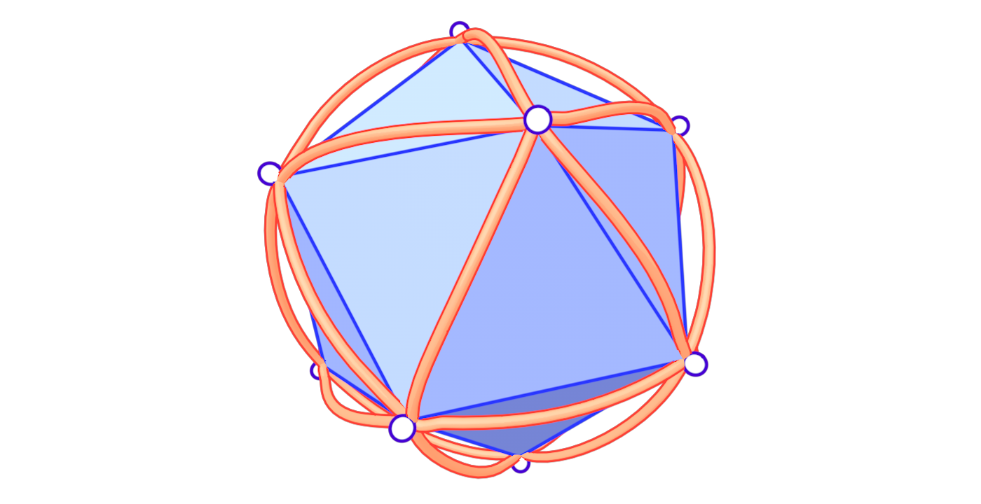
Algorithms on meshes often require some assumptions on the geometry and connectivity of the input. This can go from simple requirements like Manifoldness to more restrictive bounds like a threshold on minimum triangle angles. However, meshes in practice can have arbitrarily bad geometry. Hence, many strategies have been proposed to deal with bad meshes (see Section 2). Many of these are quite complicated, computationally expensive, or alter the input significantly. We focus on a simple, very fast strategy that improves robustness immediately for many applications, without changing connectivity or requiring sophisticated processing.

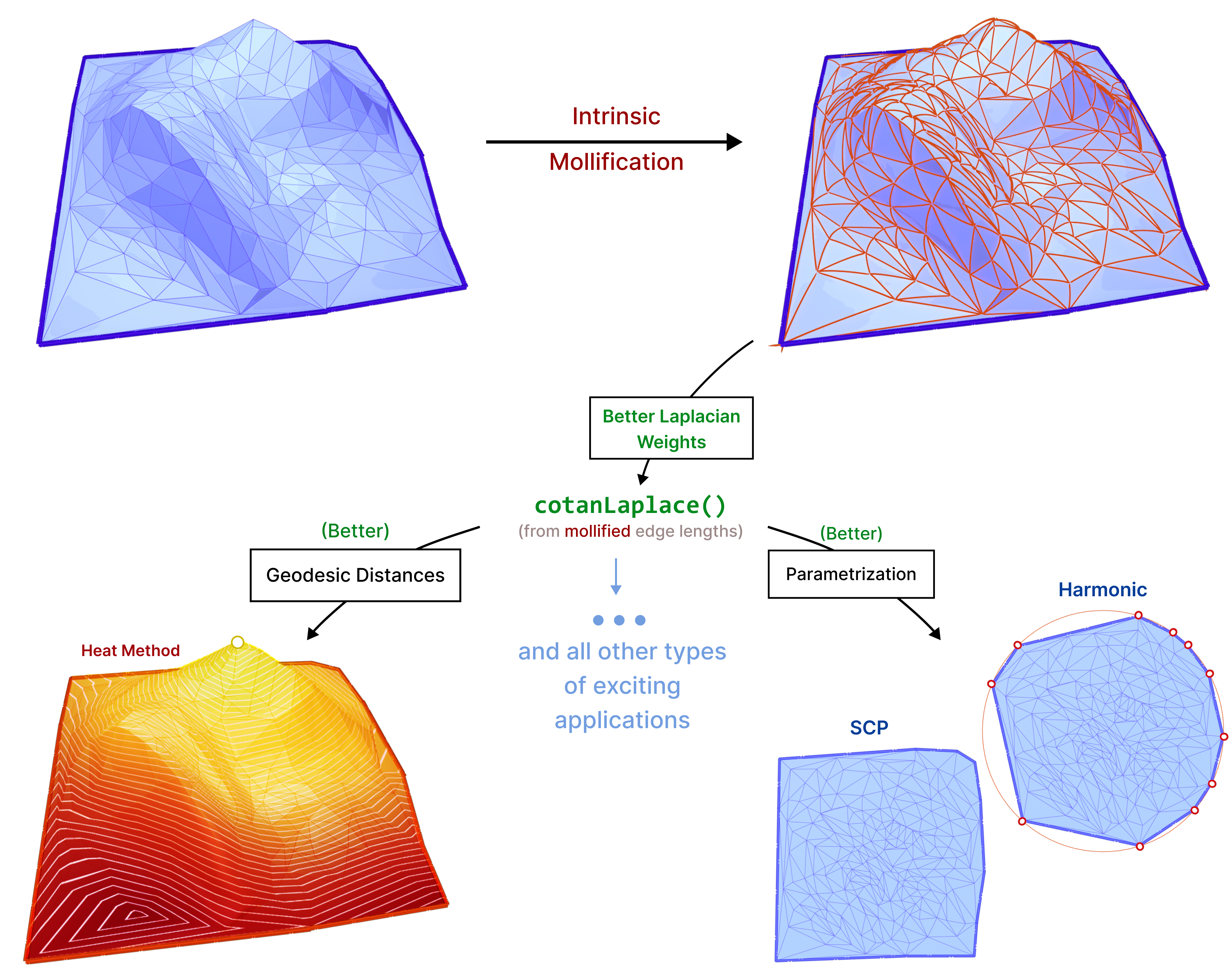
The main idea is that we can compute geometric quantities (like the Laplacian Δ) from an intrinsic representation (using edge lengths), This makes it easy to manipulate these lengths without moving vertices around, to improve triangle quality, and subsequently these computations. We introduce new schemes based on the same concept and test them on common applications like parameterization and geodesic distance computation.

Throughout this project, we mainly used Python and Libigl as well as C++, Geometry Central and CGAL for some parts.

1.1 What can go wrong?

When using the traditional formula to compute The Discrete Laplacian, many issues can arise. There are important challenges with the mesh that can harm this computation:

1. The mesh might not correctly encode the geometry of the shape.
2. Floating point errors: Inaccuracy and NaN outputs.
3. Mesh connectivity: non-manifold vertex and non-manifold edges.
4. Low-quality elements: like skinny triangles.

It is worth mentioning that (3) is addressed successfully in “A Laplacian for Nonmanifold Triangle Meshes” [1]. Throughout this project, we get deep into the challenge (4). Such elements can originate from bad scans, bad triangulations of CAD models, or as a result of preprocessing algorithms like hole-filling. A thorough analysis of bad-quality elements can be found in “What Is a Good Linear Finite Element?” [2].

1.2 What is the basic approach?

The triangle inequality states that each edge length of the three is a positive number smaller than the sum of the other two. Low-quality elements, such as the ones in the figure above, barely satisfy one of the three required triangle inequalities. For instance, if a triangle has lengths \(a, b\) and \(c\) where the opposite angle of \(c\) is very close to \(\pi\), then \(a+b\) will be barely greater than \(c\).

In a nutshell, the simple approach is to make sure that each triangle of the mesh holds the triangle inequalities by a margin. This is, for each corner in the mesh we guarantee that \(a+b>c+\delta\) for a given \(\delta > 0\). To accomplish this in each corner, we add the smallest possible value \(\varepsilon>0\) to all edges in the mesh such that \(a+b>c+\delta\) is held for each corner.

1.3 Contributions

We introduce a variety of novel intrinsic mollification schemes, including local schemes that operate on each face independently and global schemes that formulate intrinsic mollification as a simple linear (or quadratic) programming problem.

We benchmark these approaches in comparison to the simple approach introduced in “A Laplacian for Nonmanifold Triangle Meshes” [1]. We run them as a preprocessing step on common algorithms that use the Cotan-Laplace matrix. This is to compare their effect in practice. Of course, this comparison also includes comparing the effects of no mollification, and simple hacks against these schemes, as well as the effects of different parameters. This is discussed in great detail in the Experiments & Evaluation section.

2. Related Work

A large amount of work has been done on robust geometry processing and mesh repair. In particular, there have been a variety of approaches to dealing with skinny triangles. These include remeshing and refinement approaches, the development of intrinsic algorithms and formulations, and simple hacks used to avoid numerical errors.

Remeshing can significantly improve the quality of a mesh, but they are not always applicable. Naturally, they alter the underlying mesh considerably. Moreover, may not be able to preserve the original mesh topology. In addition, remeshing is often computationally expensive and may be overkill if the mesh is already of good quality except for a few bad triangles. On the other hand, Mesh refinement at least preserves the original vertices. However, it increases the number of elements significantly and is still expensive in many cases. A thorough discussion of Remeshing algorithms can be found in “Surface Remeshing: A Systematic Literature Review of Methods and Research Directions” [3].

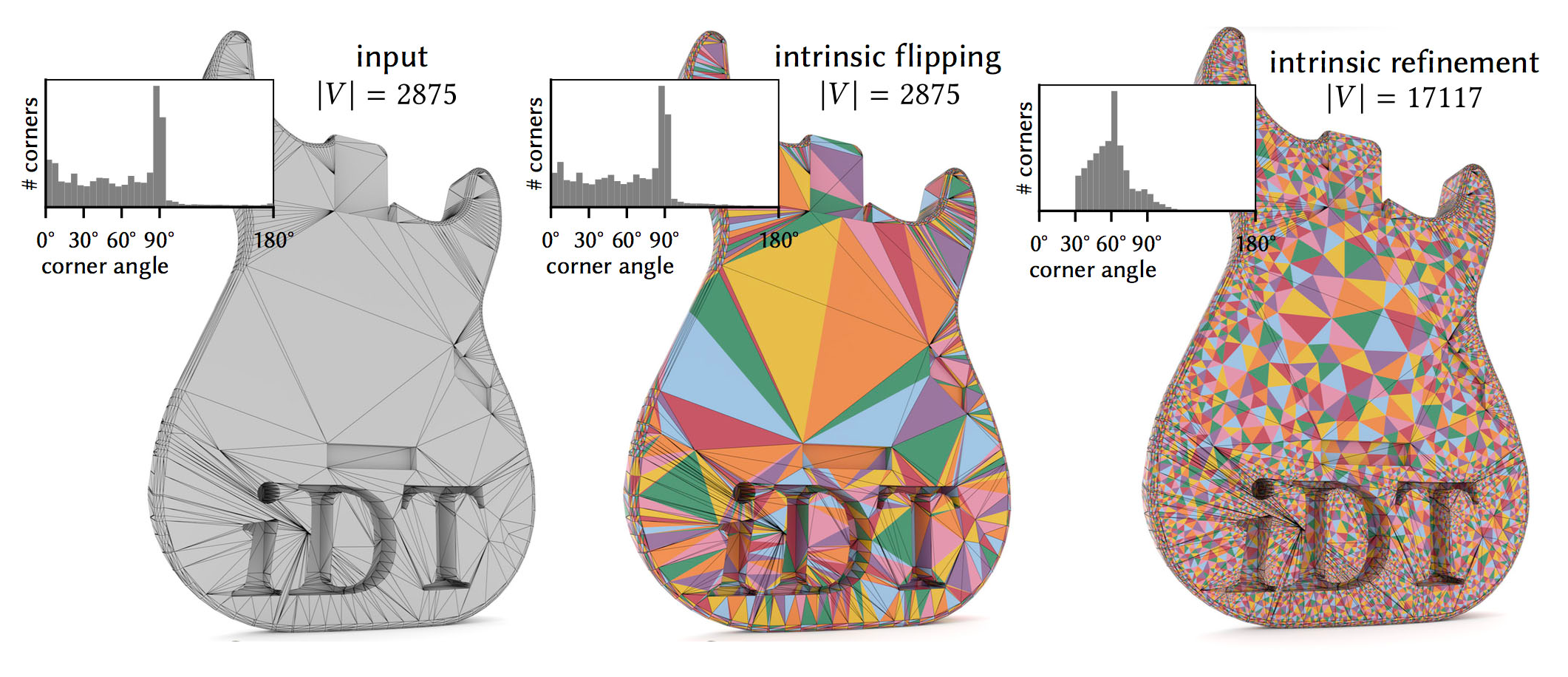
In contrast to extrinsic approaches that may damage some elements while trying to fix others, intrinsic approaches don’t need to move vertices around. For example, “Intrinsic Delaunay Triangulations” [4] using intrinsic flips can fix some cases of skinny triangles. However, it is not guaranteed to fix other cases. “Intrinsic Delaunay Refinement” [5] on the other hand provides bounds on minimum triangle angles at the cost of introducing more vertices to the intrinsic mesh. While these Intrinsic Delaunay schemes have many favorable properties compared to the traditional Remeshing and Refinement schemes, Intrinsic Mollification is much faster in case we only want to handle near-degenerate triangles. Moreover, it does not change the connectivity at all. For cases where an Intrinsic Delaunay Triangulation is required, we can still apply Intrinsic Mollification as a preprocessing step.

Lastly, Simple clamping hacks can sometimes improve the robustness of applications. But, they distort the geometry as they do not respect the shape of the elements corresponding to the clamped weights. Also, they seem to be less effective than mollification on the benchmarks we ran. They are discussed in detail in section 5.2.

3. Preliminaries

3.1 Intrinsic Triangulations

Our work is rooted in the concept of Intrinsic Triangulations. In practical Geometry Processing, triangular meshes are often represented by a list of vertex coordinates in addition to the connectivity information. However, we usually do not care about where a vertex is in space, but only about the shape of the triangles and how they are connected. So, working with vertex coordinates is not necessary and gives us information that can hinder robust computing.

Working with Intrinsic Triangulations, meshes are represented with edge lengths in addition to the usual connectivity information. In this way, we do not know where the object is, but we have all the information about the shape of the object. For a thorough introduction to Intrinsic Triangulations, see “Geometry Processing with Intrinsic Triangulations” [6] by Sharp et al.

3.2 Cotangent-Laplace Operator

Recall that the Laplace operator \(L\) acts on functions \(f:M\to\mathbb{R}\) where \(M\) is the set of vertices. For each vertex \(i\) the cotangent-Laplace operator is defined to be

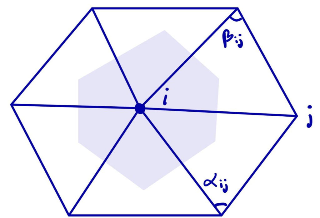
\((\Delta f)i = \frac{1}{2A_i}\sum_j (\cot(\alpha_{ij}) + \cot(\beta_{ij})(f_j – f_i)\)

The discrete Laplacian Operator is encoded in a \(|V|\times |V|\) matrix \(L\) such that the \(i\)-th entry of vector \(Lf\) corresponds to \((\Delta f)_i\). The Discrete Laplacian is extremely common in Geometry Processing algorithms such as:

• Shape Deformation.
• Parameterization.
• Shape Descriptors.
• Interpolation weights.

4. Algorithm

To solve the problem of low-quality triangles, we mollify each triangle in the mesh. By “mollify”, we mean pretending that the mesh has better edge lengths so that there are no (intrinsically) thin triangles in the mesh. Generally, for a mesh, equilateral triangles are the best to work with. If we add a positive \(\varepsilon\) value to each of the edges of a triangle, the resulting triangle will be slightly closer to an equilateral one. In fact, it will become more equilateral as \(\varepsilon\) approaches \(\infty\). However, we don’t want to distort the mesh too much. So, we find the smallest \(\varepsilon\geq 0\) such that by adding \(\varepsilon\) to each edge of the mesh we end up with no low-quality triangles. A good way to think about Intrinsic Mollification is to fix the position of each vertex of the mesh and let the edges grow to a desired length, as illustrated in Figure 5 above.

4.1 The Constant Mollification Strategy

We first recap the strategy proposed by Sharp and Crane [1]. If a triangle has lengths \(a, b\), and \(c\), the triangle inequality \(a + b < c\) holds even for very low-quality triangles. In order to avoid them, that triangle inequality must hold by a margin. This is, we ask that

\(a + b < c + \delta\)

for some tolerance \(\delta > 0\) defined by the user. Then the desired value of \(\varepsilon\) is

\(\varepsilon = \max_{ijk} \max(0, \delta + l_{jk} – l_{ij} – l_{ki} )\)

where each \(ijk\) represents the corner \(j\) of the triangle formed by vertices \(i, j, k\) and each \(l_{ij}\) represents the length of edge \(ij\).

Phase I of this project consisted of implementing this functionality. Given the original edge lengths \(L\) and a positive value \(\delta\). The function returns the computed \(\varepsilon\) and matrix \(newL\) with the updated edge lengths in the same form as \(L\).

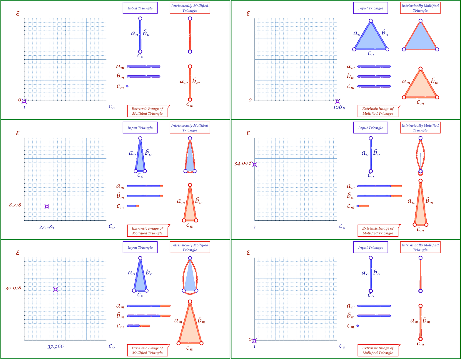
The animation above shows, for a triangle, how the mollification output changes with different \(\epsilon\) values and different lengths for the shortest edge in the triangle (\(c\) in this case). Moving forward, when comparing with other Mollification schemes, we may refer to the Original Mollification scheme as the Constant Mollification scheme.

4.2 Local Mollification

One may think that the Constant Mollification scheme is wasteful as it mollifies all mesh edges. Usually, the mesh has many fine triangles and only a few low-quality ones. Therefore, we thought it is worth investigating more involved ways to mollify the mesh.

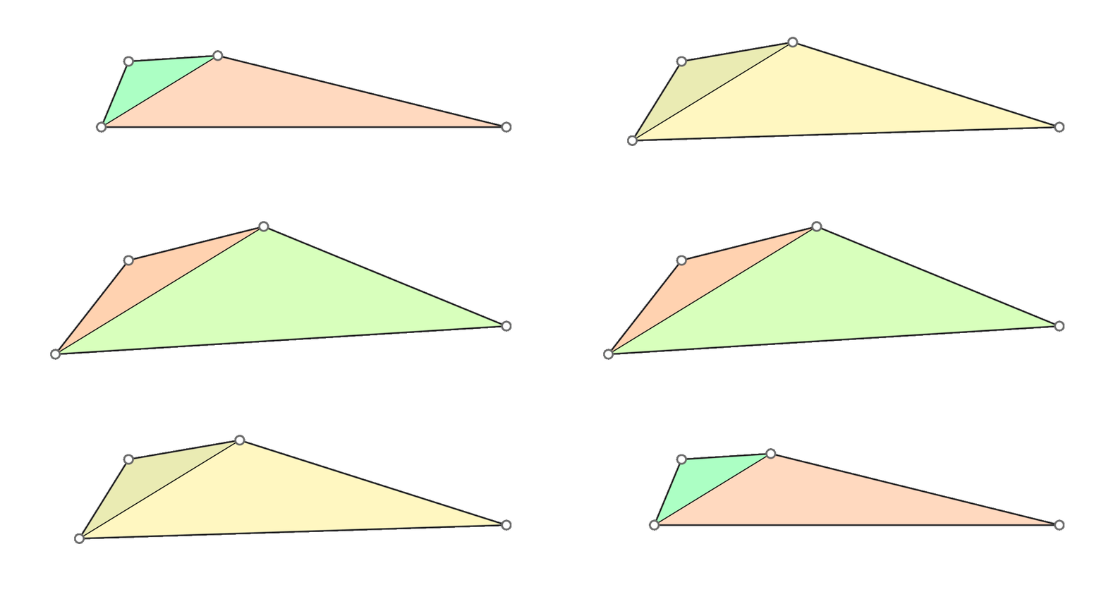
A naive approach is to go through all triangles and mollify only the skinny ones. However, while mollifying a triangle, the lengths of the adjacent triangles will change. Therefore, the triangles that were fine before may become violate the condition after mollifying the adjacent triangles. So, a naive loop over all triangles will not work, and it is not even clear that this approach will converge. The animation above shows a simple example of this case.

We had an idea to mollify each face independently. That is, we mollify each face as if it were the only face in the mesh. This breaks the assumption that the mollified length of any edge is equal on both sides of it (in its adjacent faces). The idea of having disconnected edges might be reminiscent of Discontinuous Galerkin methods and Crouzeix-Raviart basis functions.

The algorithm for this approach is basically the same as the original one, except that we find \(\varepsilon\) for each face independently. We call this approach the Local Constant Mollification scheme. Here, it might sound tempting to let \(\delta\) vary across the mesh by scaling it with the local edge length average. However, this did not work well in our experiments.

It is reasonable to think that breaking edge equality might distort the geometry of the mesh, but it is not clear how much it does so compared to other schemes as they all introduce some distortion including the Constant Mollification one. This is discussed in the section 5.3.

4.3 Local One-By-One Mollification

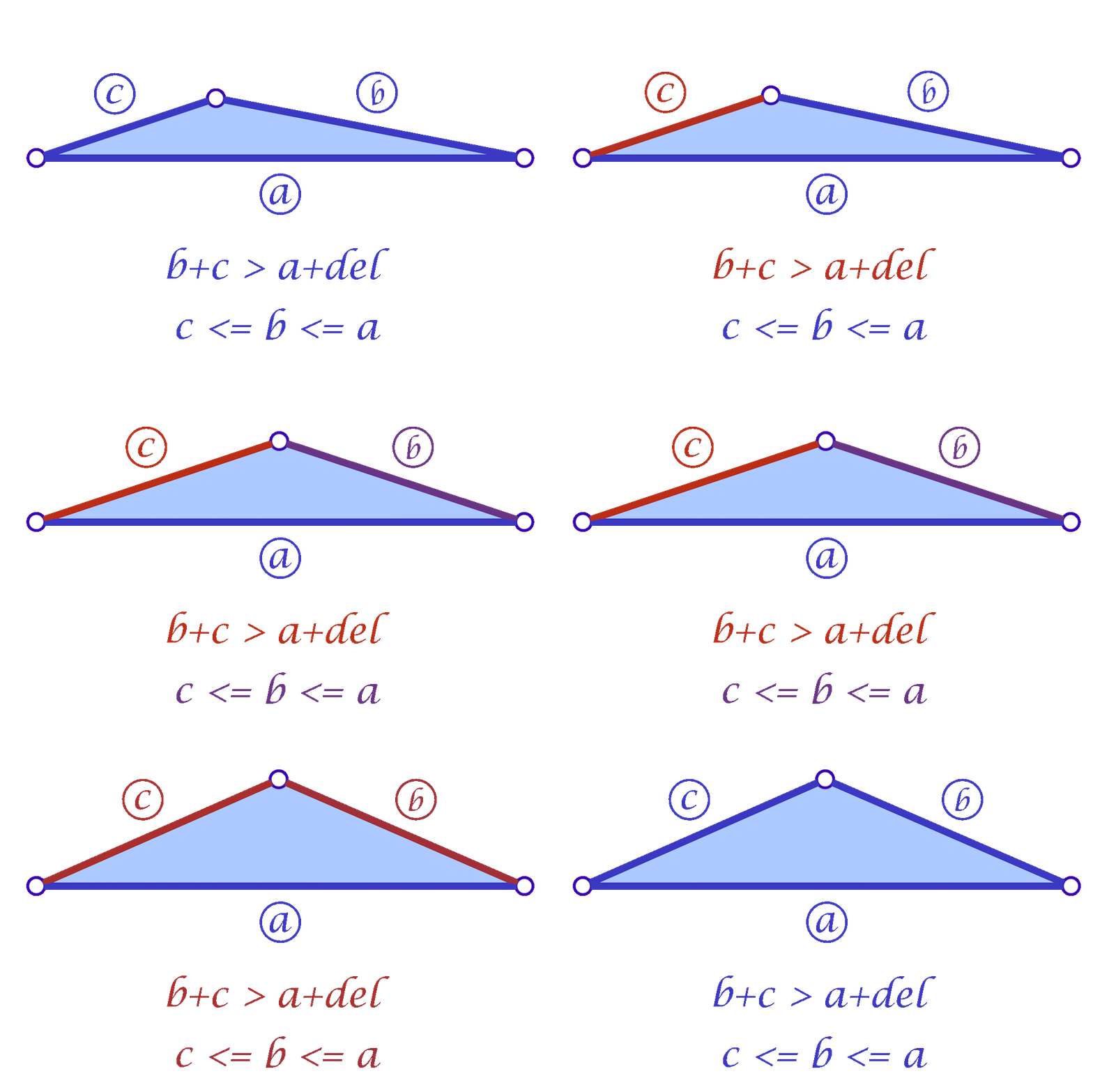
Since we are considering each face independently, we now have more flexibility in choosing the mollified edge lengths. For a triangle with edge lengths \(c \le b \le a\), one simple idea is to start with the smallest length \(c\) in the face and mollify it to a length that satisfies the inequalities described in the original scheme. To mollify \(c\), we simply need to satisfy:

\(c + b \ge a + \delta \quad\text{and}\quad c + a \ge b + \delta\)

After mollifying \(c\), it is easy to prove that we only need to keep \(a \ge b \ge c\) for the third inequality to hold. This scheme can be summarized in the following 3 lines of code:

c = max(c, b + delta - a, a + delta - b)
b = max(b, c)
a = max(a, b) 

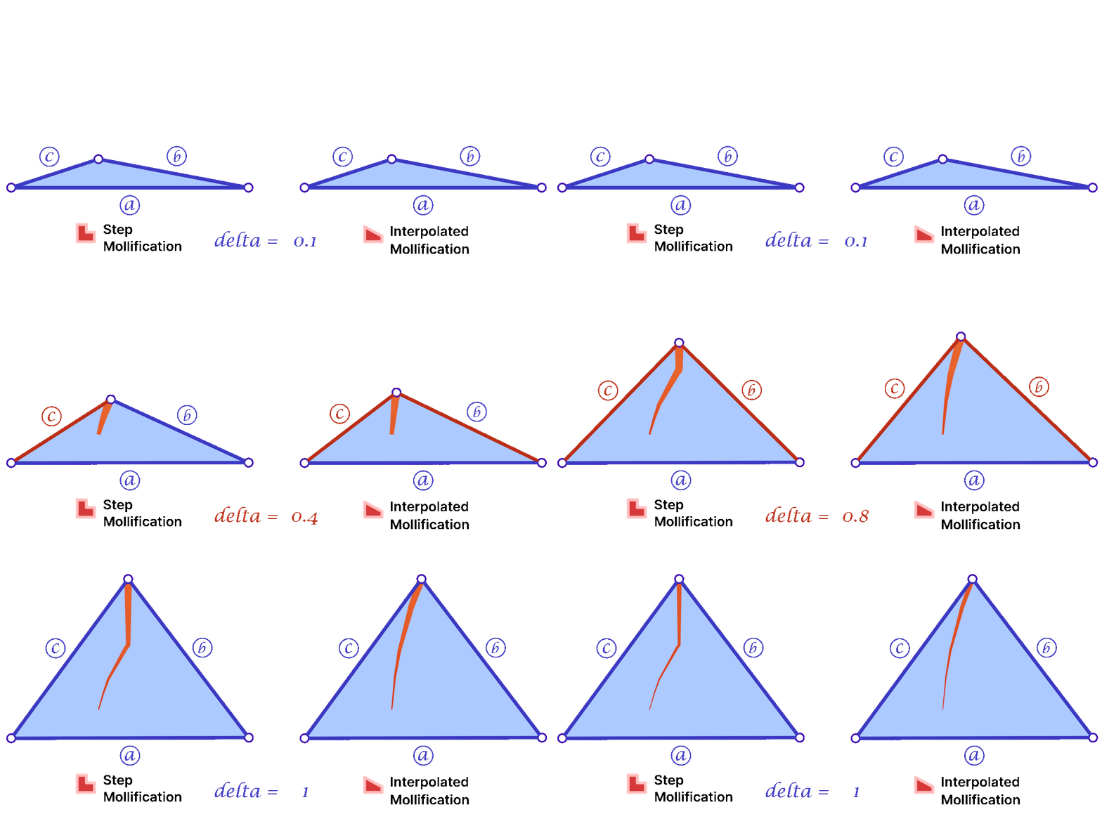
The animation in Figure 9 above visualizes this process. We call this approach the Local One-By-One (Step) Mollification scheme.

A slight variation of this scheme is to mollify \(b\) along with \(c\) to keep differences between edge lengths similar to the original mesh; this is to try to avoid distorting the shape of a given triangle too much (of course we still want to make skinny triangles less skinny). Consider the following example. Suppose the mollified \(c\) equals the original length of \(b\). If \(b\) isn’t mollified, we would get an isosceles triangle with two edges of length \(b\). This is a big change to the original shape of the triangle as shown below. So a small mollification of \(b\) even for smaller “\(\delta\)”s might be a good idea.

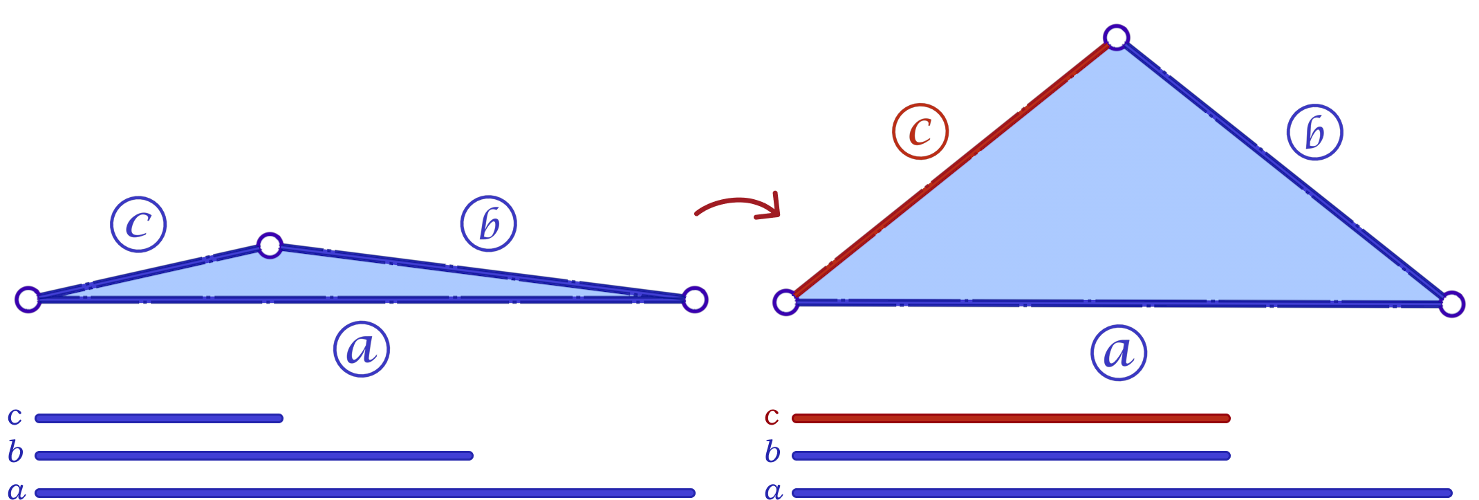
But how much should we mollify \(b\)? To keep it at the same relative distance from \(a\) and \(c\), we can use linear interpolation. That is, if \(c_o\) was mollified to \(c_o + eps_c\). we can mollify \(b_o\) to \(b_o + eps_b\) where

\(eps_b = eps_c * \frac{a_o – b_o}{a_o – c_o}\)

We call this approach the Local One-By-One Interpolated Mollification scheme. It can be summarized in the following 4 lines:

c_o = c
c = max(c, b + delta - a, a + delta - b)
b = max(c, b + (c - c_o) * (a - b) / (a - c_o))
a = max(a, b)

One more advantage of this interpolation is that it makes the behavior of \(b\) mollification smoother as \(\delta\) changes; This is visualized by the animation below.

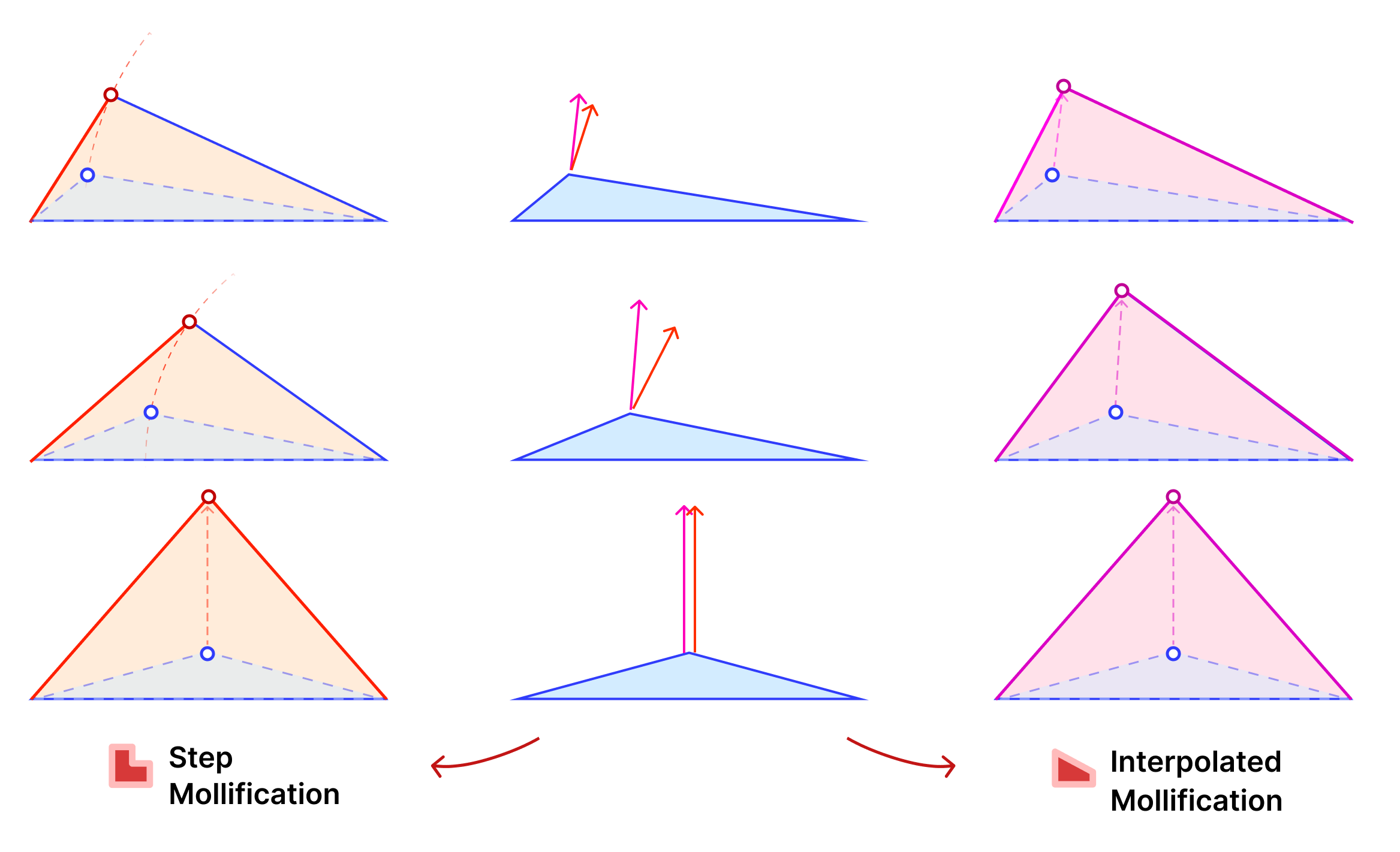
Another perspective on the behavior difference between both versions is to look at different cases of skinny triangles mollified with the same \(\delta\) value. As shown below, the Interpolated version would try to lessen the distortion in shape to keep it from getting into an isosceles triangle very quickly. Thus, having more variance in the mollified triangles’ shapes.

A great property of both schemes over the constant ones is that \(\delta\) does not need to go to ∞ in order to approach an equilateral configuration. In fact, we can prove that the mollified triangle is guaranteed to be equilateral if \(\delta \ge {a – c}\).

4.4 Local Minimal Distance Mollification

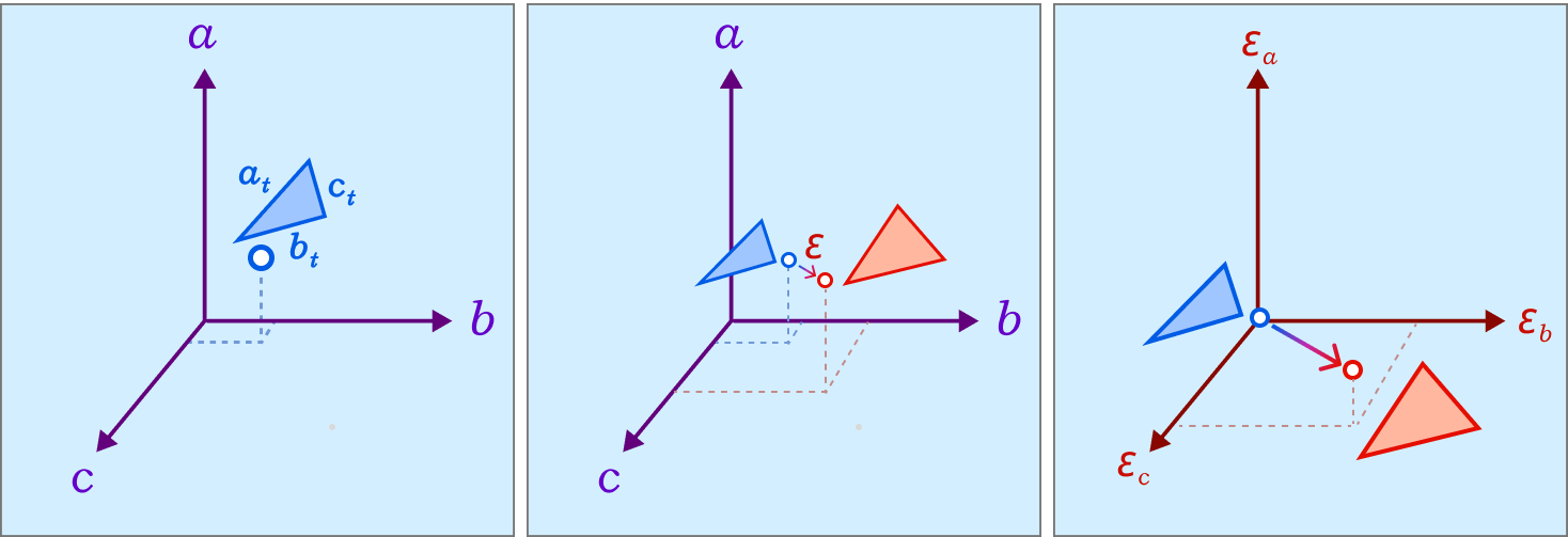
Even with the one-by-one schemes, We don’t have a guarantee that the triangle mollification is minimal. By minimal we mean that the mollified triangle is the closest triangle to the original triangle in terms of edge lengths. This is because greedy schemes don’t look back at the previous edge lengths and potentially reduce the mollification done on them.

A good result from working with intrinsic lengths is that it is easy to deal with one triangle at once if we think about each edge as an independent variable. Then, the original triangle is a point in the space of edge lengths and the mollified triangle is another one. Since we are only adding length, it is easier to think of the original triangle as the origin point of this space and all vectors would represent the added length to each edge. Thus, the 3 axes now represent each edge’s \(\epsilon\). This is illustrated in the Figure above.

The problem of finding the minimal mollified triangle is then a problem of finding the closest point to the original triangle in this space inside the region defined by 6 constraints (triangle inequalities & non-negativity of epsilon). These make up a 3D polytope as shown below.

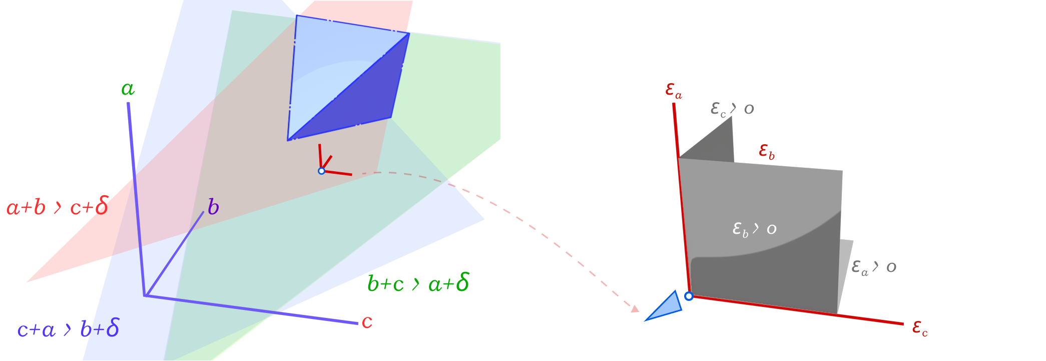
Depending on how we define the distance between two triangles, this problem can be solved using Linear Programming or Quadratic Programming. We can define the distance between two triangles as the sum of the distances between each corresponding edge of both triangles, this distance is just the \(L_1\) norm (Manhattan) of the difference between the edge lengths of the two triangles. This is a linear function of the edge lengths. Therefore, the problem of finding the minimal mollified triangle is the following Linear Programming problem:

\(\begin{gather*}
\text{min} \quad
I_{3 \times 1} \cdot x \\
\\
\text{s.t.} \quad
\begin{pmatrix} 1 & 1 & -1 \\ 1 & -1 & 1 \\ -1 & 1 & 1 \\ 1 & 0 & 0 \\ 0 & 1 & 0 \\ 0 & 0 & 1 \end{pmatrix} x =
\begin{pmatrix} \delta \\ \delta \\ \delta \\ 0 \\ 0 \\ 0 \end{pmatrix} \\ \end{gather*}\)

The first 3 rows correspond to the 3 triangle inequalities, and the other 3 restrict mollification to positive additions to the length.

In the other case, where we define the distance between two triangles as the \(L_2\) norm (Euclidean) of the difference between the edge lengths of the two triangles, the problem of finding the minimal mollified triangle is a Quadratic Programming problem. The constraints are still the same, the only difference is that we minimize \(x^T x\) instead of \(I_{3 \times 1} \cdot x\). The good news is that both problems can be solved efficiently using existing solvers. The figure above visualizes both concepts.

With these 2 versions, we have two more schemes, namely, the Local Minimal Manhattan Distance and the Local Minimal Euclidean Distance mollification schemes

4.5 Sequential Pooling Mollification

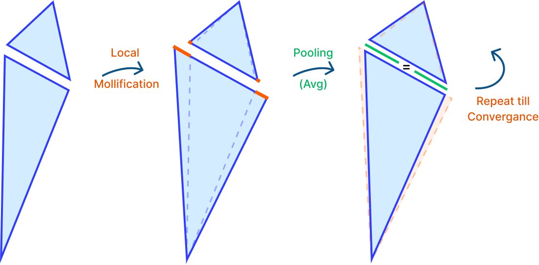
After exploring a lot of different local mollification schemes, we thought it would be a good idea to try to get the advantages of local mollification schemes (like significantly reducing the total mollification) while still keeping the edge lengths on both sides equal. The first idea that came to mind was to mollify the mesh using local scheme, and then average the mollified edge lengths on both sides of each edge. And repeating this process until convergence. The figure above visualizes this idea.

When we tried this idea on a few meshes, we noticed that the mollification process was not converging. We tried other pooling operations like Max, Min, and combinations of them. Unfortunately, none of them were converging. It might be worth it to put some time into trying to derive different pooling functions with convergence guarantees.

4.6 Global Optimization Mollification

In the search for a scheme that has a lot of the good properties of the local schemes, while keeping edge lengths on both sides equal, we took the idea of finding the closest mollified triangle to the original triangle in terms of edge lengths, but instead of doing it locally, we will apply the problem to all mesh edge lengths at once.

This also involves solving a Linear Programming or Quadratic Programming problem based on the distance function we choose. We call the global versions the Global Minimal Manhattan Distance and the Global Minimal Euclidean Distance Mollification. Effectively, this is finding the least amount of mollification while not breaking the equality of edge lengths on both sides.

4.7 Post-mollification Normalization

Since we are always adding length in mollification, Properties that aren’t scale invariant might get scaled. In order to avoid this, we might want to scale the mollified edge lengths down so that the total surface area is the same. This would not make a difference for the Cotan-Laplace Matrix but it can a difference for the Mass Matrix (among other things).

For some applications, it would make sense that we want a different quantity to remain unchanged after the mollification. For example, To keep the geodesic distances from getting scaled up, we can normalize the mollified edge lengths so that the total edge length is the same after mollification. for each mollified edge length \(e^i_{mol}\):

\(e^i_{mol}- = e^i_{mol} * \frac{\sum_{j = 1}^{|E|} e^j_{mol}}{\sum_{j = 1}^{|E|} e^j}\)

We implemented this step in our C++ implementation and used it in the Geodesic Distance Benchmarks in.

5. Experiments and Evaluation

5.1 Data Sets for Benchmarks

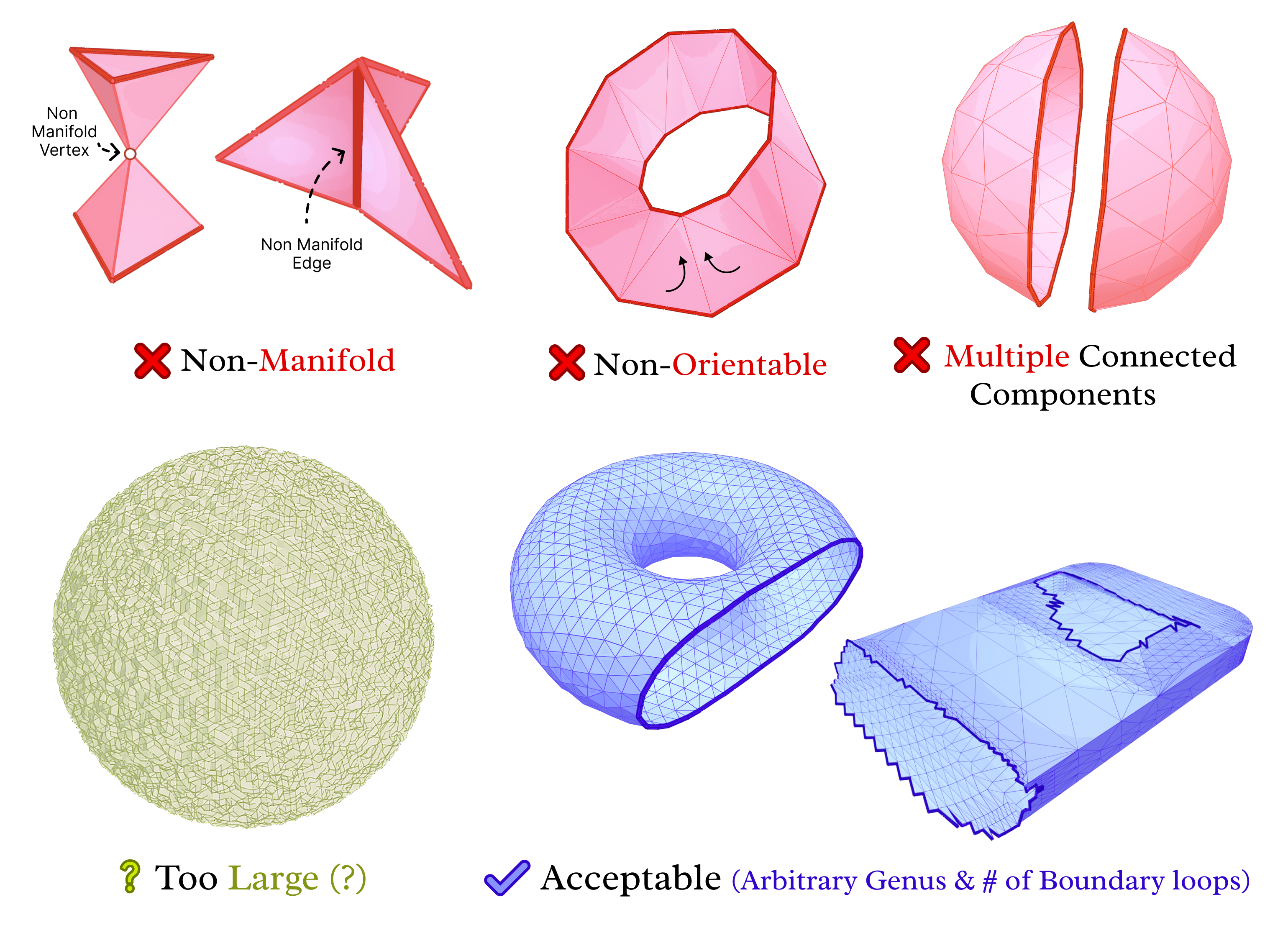
For most experiments, we use the Thingi10k data set [8]. It is composed of 10,000 3D models from the Thingiverse. The models have a wide variety of triangular meshes. This variety comes in regards to Manifoldness, genus, number of components and boundary loops, and more. A lot of the meshes also have very bad quality triangles. So, it is suitable for testing our work on a wide range of scenarios.

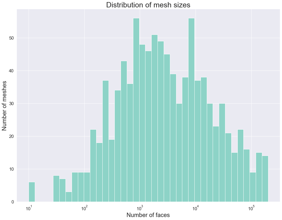
We implemented a script to filter the data set. In particular, we removed not manifold, multiple-component, and non-oriented meshes. The remaining meshes are categorized based on the size of the mesh and the number of skinny triangles (i.e. ones that violate the mollification inequalities). This step was very helpful for testing and debugging the different aspects of the proposed work quickly by choosing the appropriate meshes. The Figure above shows examples of acceptable and filtered-out meshes. For most of the benchmarks, we used this filtered data set . In some cases, we filtered out large meshes (i.e. \(\|F\| > 20,000\) triangles) to reduce the running time of the experiments. The graph below shows the (log) distribution of the number of faces used for some of the benchmarks.

In search for other data sets to evaluate the proposed work, “A Dataset and Benchmark for Mesh Parameterization” [9] has an interesting set of triangular meshes used to benchmark parameterization schemes. As described, Thingi10k meshes come from real data, usually used for 3D printing and video game modeling but the data is not particularly suitable for testing parameterization methods. Since mollification will be important for parameterization methods, the investigation of further data sets is needed.

“Progressive parameterizations” [10] presents a data set which has been used before in the literature for benchmarking parameterization methods. However, [10] data is composed of meshes based on artificial objects. In this case, [9] obtain and makecorrection corrections on meshes from multiple sources, including the Thingiverse, which are mainly obtained from real-world objects and form the set called Uncut. Then, in possession of the Uncut, they perform cuts along the artist’s seam to form the set called Cut. . Due to time limits, The parameterization benchmarks currently reported are still on Thingi10k (with some work to extract patches). But, it may be worth it to use Cut for the parameterization benchmarks in the future.

5.2 Alternative Strategies

The effects of badly shaped triangles have been present since the early days of mesh generation. A common appearance of these effects is on Surface Parameterization Problems. Examples of these problems are the Least Squares Conformal Mapping and Spectral Conformal mapping, which essentially are composed of vertex transformations whose weights are in their essence non-negative. However, it is known that very thin triangles can result in parameterization weights that are negative or numerical zeros which need to be avoided.

In practice, simple heuristics have been applied to avoid non-positive conformal map weights. These are indeed simple in nature but known to be in some cases effective

1. Replace negative weights with zero, or with absolute value
2. Replace NaN & infinity weights with zero, or with one.
3. Replace numerical zeros with zero.

We tried using some of these hacks and even combinations of them. Hence, Some of them turn out to be more useful and produce better results. For example, for the parameterization benchmarks, the negative replacement hacks were not useful at all. On the other hand, the NaN (& Infinity) replacement hacks are much more useful. Also, the near-zero approximation hack improves things sometimes but makes things worse more often. Overall, it is not immediately clear if any of them are better in a general sense.

For this, given an appropriate measure to be discussed in the mapping benchmarks in section 5.5.4, the Mollification schemes are compared to the best-performing combinations of these simple heuristics.

5.3 Comparison of Mollification Strategies

5.3.1 Length Distortion

First, we compare all schemes’ performance independent of any application; to see how much they affect the mesh geometry. For each mesh in Thingi10k (filtered), we compute the relative total difference between the mollified and original lengths. These differences are averaged over all meshes and reported as Avg. Added Length as a metric of length distortion. We also report the average percentage of mollified edges (for global schemes, it can not be counted explicitly).

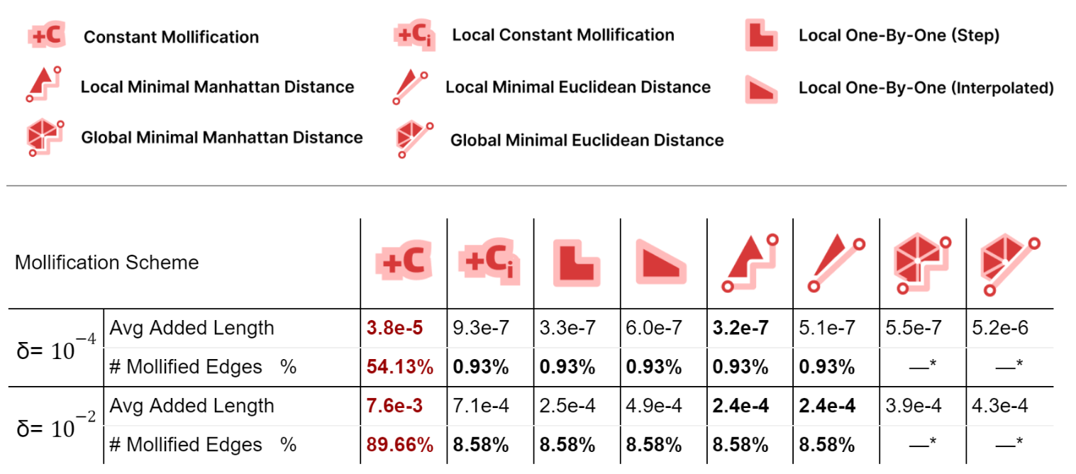
Local schemes introduce much less mollification than the constant one as they only mollify near-degenerate faces, especially for smaller \(\delta\); due to having less strict inequalities and thus less faces violating them. The number of mollified edges is x50 times smaller for local schemes.

For the average added length, Unsurprisingly, The Local Minimal Manhattan distance scheme is always optimal. For the Euclidean distance version, it has more added length because the metric we are reporting is essentially a scaled sum of Manhattan distances for each face. Additionally, the Local 1-by-1 Step scheme is always very close to the Local Minimal Manhattan distance scheme as in most cases, we only need to mollify one edge. In such cases, Both schemes behave identically.

Compared to the step version, the Local 1-by-1 Interpolated scheme allows some more length distortion for smoother behavior over \(\delta\) values and better triangle length ratio preservation. Moreover, this distortion is still quite low compared to the Local Constant scheme.

The Global Minimal distance schemes have significantly less added length than the constant one, and more than the local analouges. But, they have the benefit of keeping the 2 sides lengths of an edge equal. The Euclidean version has a strangely larger added length than the Manhattan one for \(\delta = 10^{-4}\). This might be worth investigating further.

More than 50% of the dataset needs mollification even for forgiving \(\delta\) values, which shows that skinny triangles are common in practice. This motivates the development of mollification and other preprocessing step.

5.3.2 Time Performance

It is important to also analyze the time performance of these schemes. The table below shows the average running times for the filtered dataset meshes with \(\|F\| \le 200,000\).

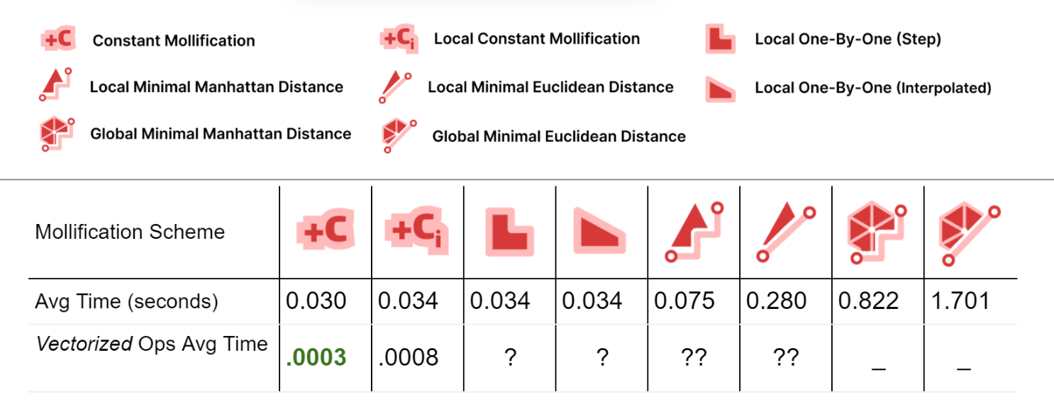
First, comparing the basic implementations (With no vectorized NumPy Operations), we see that most of the local schemes have very similar running times to the constant scheme (the fastest). This is great news because the extra steps implemented in them don’t have a large impact on the average running time.

For the Local Minimal distance schemes, they are a bit slower. But it is important to note here that we didn’t try to find the most efficient libraries for linear programming and quad programming optimizers; In fact, we used a different one for each problem (Scipy and Cvx-Opt respectively). So, for a more careful performance analysis, it would be worth trying different libraries and reviewing the implementation. It can also be beneficial to try to find a simple update rule form for them (similar to the implementation of the greedy ones). From the first glance, it sounds feasible, especially for the linear program version as it is extremely similar to the 1-by-1 step scheme.

For the global minimization schemes, they are much slower than the others. Here, the notes mentioned above about efficient optimizers also hold.

To improve the running times, we implemented the Constant scheme and the local Constant schemes using NumPy’s vectorized operations. It is clear that this made a huge difference (about x100 and x40). We didn’t have time to try to do the same for the other local schemes. But it might be achievable and it would be interesting the resulting boasts. Moreover, the local schemes are very easy to parallelize which is one more way to optimize them. Since the local schemes’ time is mostly spent iterating over the faces and checking them, they can be integrated into the Laplacian computation loop directly to save time.

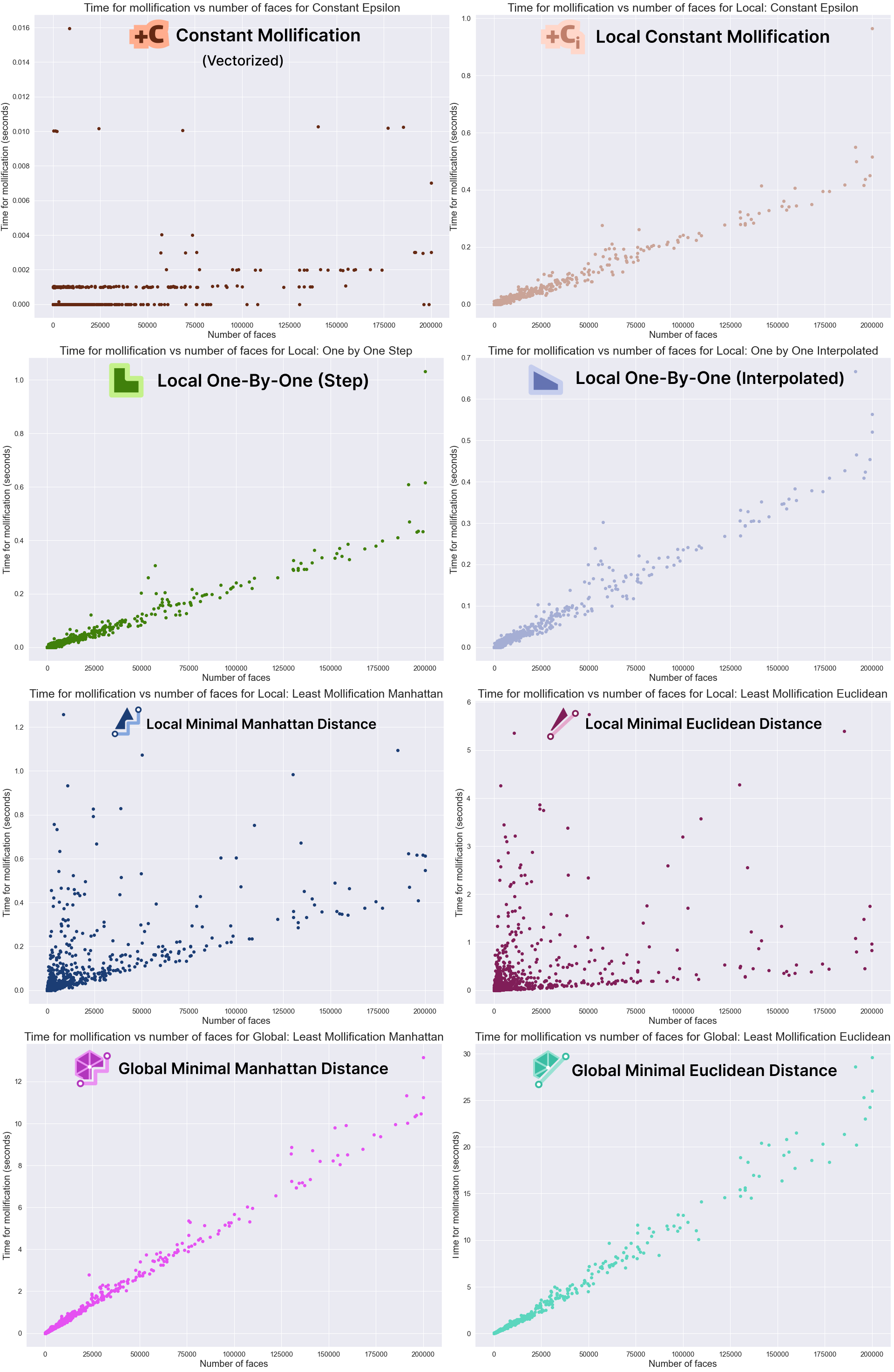
The graphs above show that the Mollification schemes have a linear running time in relation face counts. Indeed, this is obvious for the local schemes as each face is processed independently. The local minimal distance schemes uniquely have very high variance, it is not as clear why this happens, though. For the vectorized implementation of the constant scheme, the running time is too small to be able to draw a pattern. Finally, although the global schemes also have linear growth, they are too slow in comparison. For example, a mesh with about 200,000 faces would take about 10 seconds for the Manhattan version and 25 for the Euclidean distance version on average. It is not clear how much performance gain we would get from a more optimized implementation with more efficient libraries.

5.4 Mollification + Simple Applications

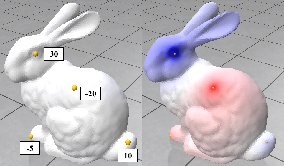
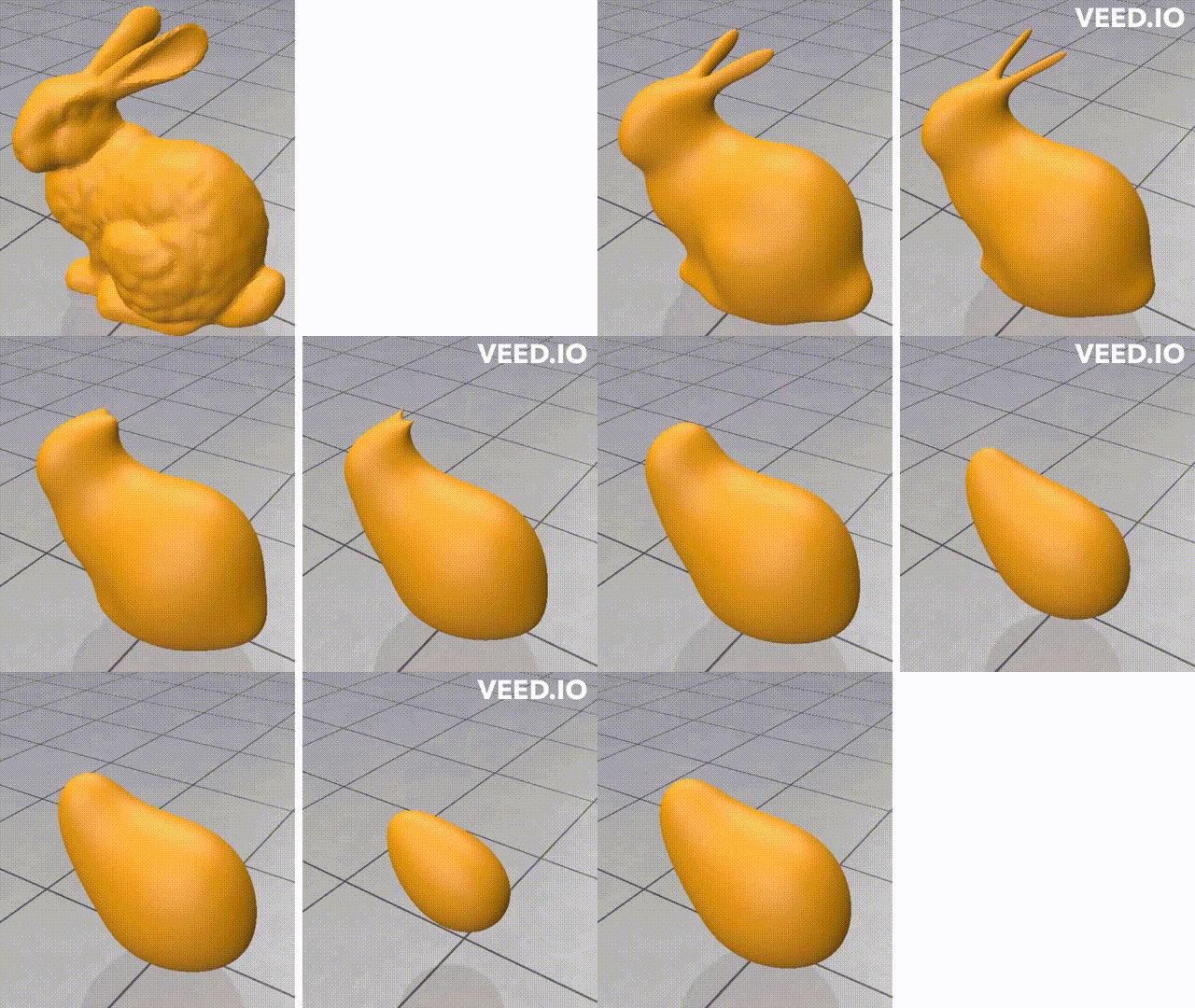
Here we try 2 simple algorithms that use the Cotan Laplacian and the Mass matrix. The first is solving a simple Poisson equation that finds a smooth density function over the mesh vertices given some fixed density values on a few of them. The other one is the “(Modified) Mean Curvature Flow” [11]. This flow is used for Mesh Smoothing. the Figures above show these algorithms’ output on the stanford bunny mesh.

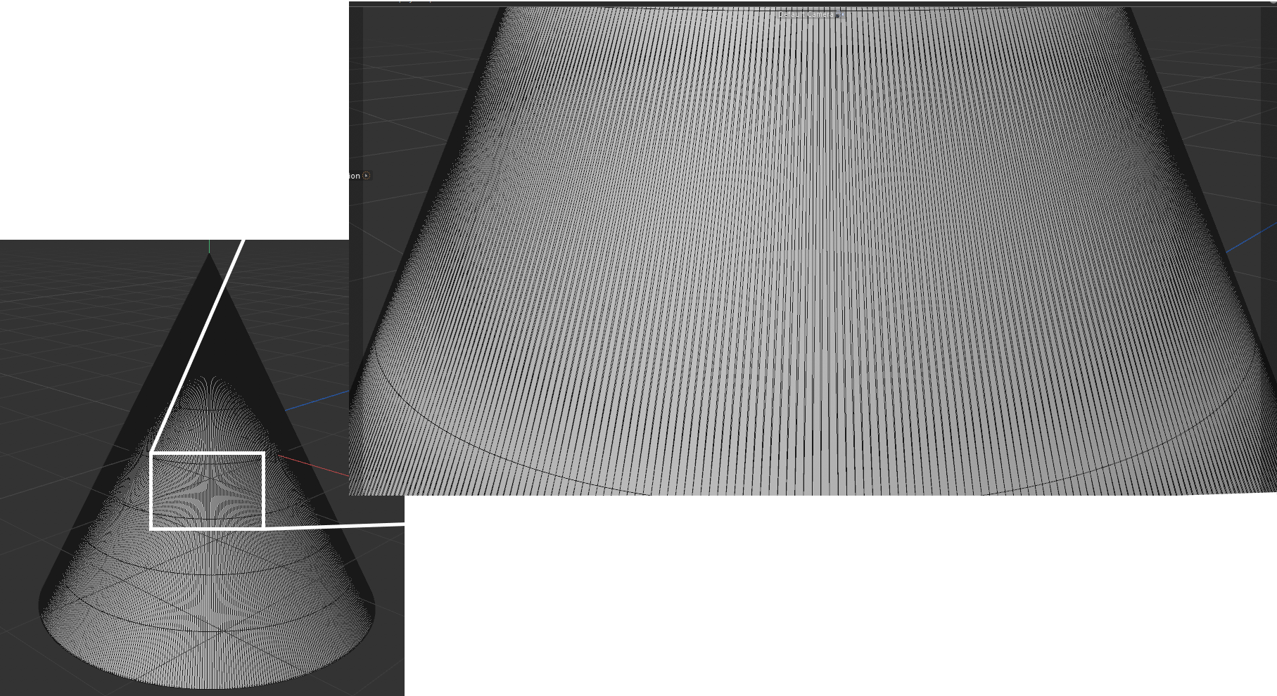
For purposes of quickly testing some applications with and without mollification, we generated a simple cone mesh segmented as, Rotation segments = 500, Height segments = 8, Cap segments = 8 (Shown above). Even though this is a mesh with simple shape and connectivity, it has a lot of skinny triangles. Without Mollification, running both algorithms on this mesh results in NaN values over the whole mesh. But with the slightest bit of Mollification (extremely small \(\delta\) values like \(10^{-10}\)), the algorithms don’t crash and we can see reasonable results as shown below.

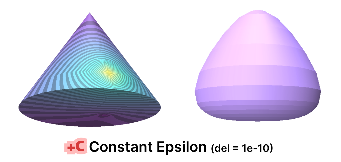
It is worth noting that some combinations of the hacks earlier also produced similar results, some produced NaNs and others produced some results that are much less accurate. In general, it is not always clear which combination makes sense for the problem at hand.

5.5 Surface Parameterization

5.5.1 The Parameterization Problem

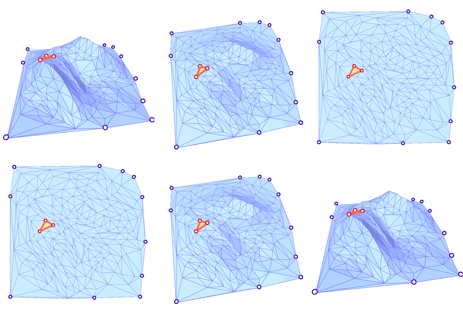
As defined by “Least squares conformal maps for automatic texture atlas generation” [12], the problem of parameterizing a surface \(S \subset \mathbb{R}^3\) is defined as finding a correspondence between \(S\) and a subset \(S’ \subset \mathbb{R}^2\) by unfolding \(S\). The animation above visualizes this “unfolding”. When the map \(f: S \to S’\) locally preserves the angles, the map is said to be conformal.

5.5.2 Relevant Parameterization Algorithms

In order to preserve angles between \(S\) and \(f(S)\), it is possible to minimize the variation of tangent vectors from \(S\). From [12], we can define an energy \(E_{LSCM}\) based on vector variation and the variance prediction method of Least Squares, the energy of Least Squares Conformal Map as follows:

\(E_{LSCM}(\textbf{u}, \textbf{v}) = \int_X \frac{1}{2} | \nabla \textbf{u}^\perp – \nabla \textbf{v} |^2 dA \)

As discussed by “Spectral Conformal Parameterization” [13], the previous equation can be written in matrix form. Let \(L_c\) denote the cotangent Laplacian matrix and \(\textbf{u}, \textbf{v}\) be vectors so that \([\textbf{u}, \textbf{v}]^T A [\textbf{u}, \textbf{v}]\) is the area vector of the mesh, we have the LSCM energy as:

\( E_{LSCM}(\textbf{u}, \textbf{v}) = \frac{1}{2} [\textbf{u}, \textbf{v}]^T (L_c – 2A) [\textbf{u}, \textbf{v}]\)

Hence, in order to minimize this energy, the gradient must be zero, that is, \(Ax = 0\). However, since trivial solutions can be found in this optimization, two methods are used: pinning vertices and principal eigenvector of the energy matrix.

The idea of pinning two vertices is that one vertex will determine the global translation, while the other will determine the scaling and rotation, avoiding zeros in the Least Squares method. The other approach is to find the two smallest eigenvalues and eigenvectors of the energy matrix. Since a trivial solution is possible, the smallest eigenvalue is zero, then the second smallest eigenvalue and corresponding eigenvector will produce the minimization in question. The latter is a method called Spectral Conformal Parameterization (SCP). Both are shown in Figure. 25 above.

We also consider Harmonic Parameterization. This method is based on the idea of solving the Laplace equation on the surface \(S\) with Dirichlet boundary conditions. That is, given a surface \(S\) with all boundary vertices pinned, the Laplace equation \(\delta z = 0\) is solved on the interior of \(S\). Solving this equation results in a minimal surface as shown above.

Now, if we pin the boundary vertices to a closed curve in the plane, the resulting minimal surface would also be planar and the solution is the parameterization. In fact, since all boundary vertices are pinned, minimizing the harmonic energy is equivalent to minimizing the conformal energy mentioned above as the signed area term is constant for all possible parameterizations of \(S\).

In all of our experiments, we pin the boundary vertices on a circle. The relative distances between consecutive boundary vertices are preserved in the parameterization. A Harmonic Parameterization of the same mount model is shown below side-by-side with LSCM and SCP.

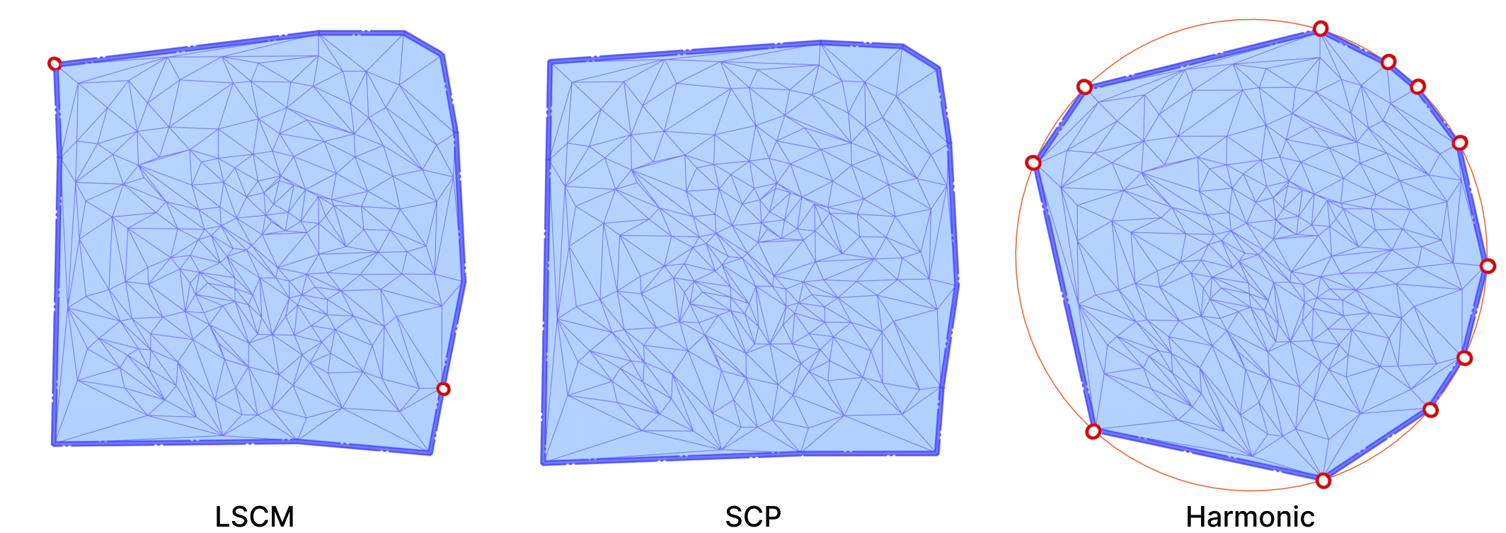
All three algorithms use the cotangent Laplace matrix in their energy minimization process. Computing this matrix involves edge lengths and triangle areas. Therefore, they are good candidates for testing the effects of mollification when applied to bad meshes.

5.5.3 Evaluation Metrics & Methodology

In order to produce a technical comparison between the alternative hacks defined in Section 5.2 and Intrinsic Mollification, adequate measures are necessary. For this, we measure Quasi-conformal Distortion. This error metric (visualized below) is a measure of angle distortion for a given mapping and it is usually used to measure the quality of a Conformal Parameterization.

A best-case transformation is a triangle similarity. That is, shearing should be avoided to abstain the parameterization from distortion. For this, the Quasi-Conformal (QC) Error measures how close the original and final triangles are to a similarity. An error of \(QC=1\) means that no shear happened. This can be used for comparing the distortion between the alternative strategies and the mollification.

For harmonic parameterization, we measure the relative area and length distortion instead of the QC error metric. This is because harmonic parameterization is not Conformal. Specifically, for one mesh, we compute this error as the norm of the vector of the (L1) normalized area (or length) differences before and after parameterization. In other words:

\(e_{A} = | \frac{A_{param}}{|A_{param}|_1} – \frac{A_{o}}{|A_{o}|_1} |\),

\(e_{L} = | \frac{L_{param}}{|L_{param}|_1} – \frac{L_{o}}{|L_{o}|_1} |\)

Here, \(A_{param}\) is a vector of face areas after parameterization (and potentially mollification), and \(A_{o}\) is the same but of the original mesh. We normalize each before taking the difference to make sure the total area is equal. The norm of this difference vector is the metric we compute to see how areas are distorted. We also compute an isometry error metric which is computed in the same way but over lengths instead of areas.

Whenever the Laplacian has weights that are either negative or numerical zeros, it is common for a parameterization to produce flipped triangles. That is, a triangle which intersects other faces of the parameterized mesh. Then, a possible measure is to count the number of flipped triangles in the parameterized form. We tried this on a few meshes (but not across the dataset) to see how much mollification improves things and we found some promising results. It is worth trying this on a large-scale dataset to get more specific statistics in the future.

Parameterization requires the input mesh to have at least a boundary loop. It also zero genus (i.e. topologically equivalent to a sphere). Since most Thing10k meshes are solid objects with arbitrary genera, we implemented a simple algorithm to extract a genus-zero patch from the input mesh.

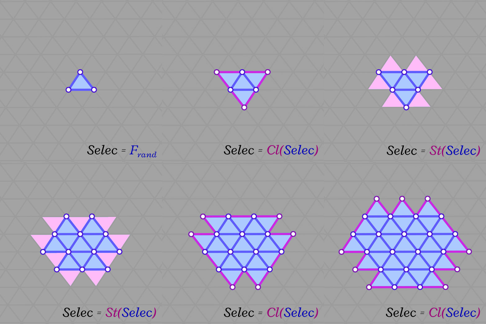
The algorithm is a simple Breadth-First-Search starting from a random face and visiting neighboring faces. This is equivalent to growing the patch by applying the \(Star\) and \(Closure\) operators (\(Closure \circ Star\)) repeatedly (as shown below). The algorithm stops when we reach a specified fraction of the total number of faces in the input mesh. Of course, this algorithm is not guaranteed to find a manifold genus-zero patch, but it is not costly to re-run it (with a bit smaller fraction and from a different face) until a valid patch is found. Most patches are found on the first or second try.

5.5.4 Benchmark Results

We ran the Conformal Mapping algorithms on the filtered Thingi10K dataset (~ 3400 meshes) and with with \(\delta\) values \(10^{-4}\) and \(10^{-2}\). We report the median of Quasi-Conformal (QC) errors across all meshes as well as the number of times this metric function returned NaN or Inf values (indicating degenerate parameterizations like zero-area). The table below summarizes such results

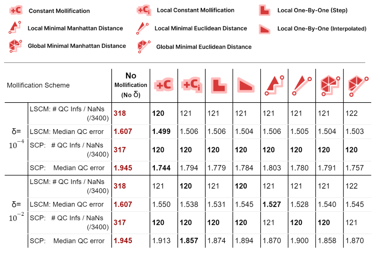
We immediately see an improvement in robustness. For all schemes and both mapping algorithms, about 62% of the cases where QC = NaN (or inf) were solved by mollification. This is independent of the chosen \(\delta\) value. Of course, in some of these cases, it could be the case that our implementation of the QC error function is not robust enough (other than the mapping itself). But the effect of Mollification is clear nonetheless.

As for the QC error values, most schemes are generally close (and much better than no mollification), with the constant scheme being slightly better with smaller deltas and slightly worse with larger deltas. Overall, the more advanced schemes do not seem to make things better than the basic (constant) one for Conformal Parameterization. Here, it seems that smaller \(\delta\) values like \(10^{-4}\) seem to work better than larger values (\(10^{-2}\)).

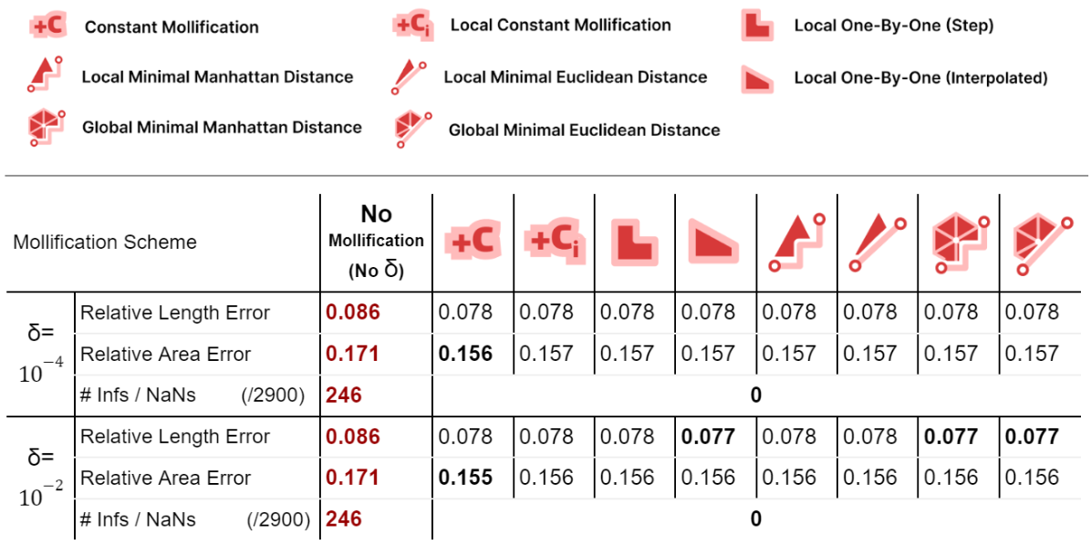
For harmonic mapping, all cases where the length error or area error where NaNs (or infinities) were solved by all schemes. As for the relative length and area errors, they seem to also improve significantly with mollification. And comparing the mollification schemes, they seem extremely close as well. Overall, ther isn’t a clear advantage of one scheme over the others.

We also ran benchmarks to compare these mollification schemes against the hacks. We first ran a small sample of the dataset on all combinations of the hacks mentioned in 5.2. There have been only two options that seemed to improve things significantly here. Namely, Replacing NaN/Infs with zeros or with ones. So, we ran the parameterization benchmarks again (on 3400 meshes) with these two options and without them, and compared that against 4 of the mollification schemes (\(\delta = 10^{-4}\)). The results are summarized in the table below.

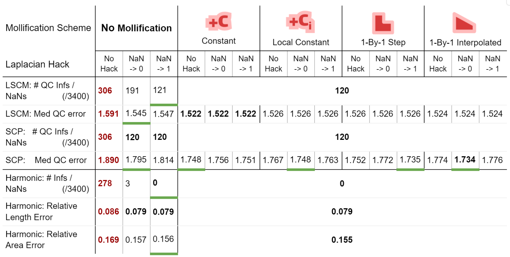
From the table, first, we see that the Nan-to-Zero hack isn’t reducing the cases of Qausi-Conformal error nearly as much as the Nan-to-One hack or the mollification schemes. Moreover, while both hacks reduce the Median of these errors, there is a clear advantage for all Mollifiction schemes. In fact, all of them reduce this metric by about \(~ 50-60\%\) more on average than the hacks. From this, it is clear that Intrinsic Mollification has stronger effects on robustness than even the best-performing combinations of the tested hacks.

Another surprising result from the table is that combining Intrinsic Mollification with such simple hacks can be useful in some cases. For example, on local schemes in the table, the hacks sometimes even further improve the effect of mollification on the QC error. This shows that we can still use hacks after Mollification but it is not immediately clear when to use which hack because they can also harm the results.

Overall, for the parameterization benchmarks, there does not seem to be a clear advantage of the introduced Mollification schemes to the original constant one.

5.6 Geodesic Distance

5.6.1 The Geodesic Distance Problem

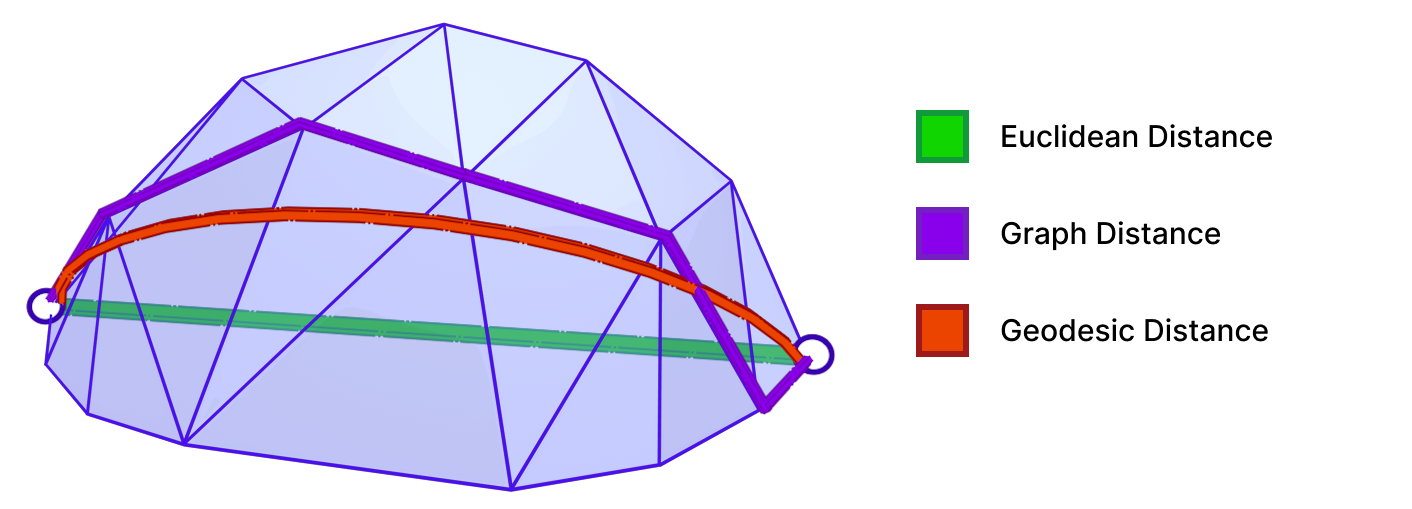
A Geodesic path represents the shortest (and straightest) path between two points on a surface. Geodesic distance is the length of such path. As shown above, the geodesic distance is different from the trivial Euclidean distance. Accurate computation of geodesic distance is important for many applications in Computer Graphics and Geometry Processing, including Surface Remeshing, Shape Matching, and Computational Architecture. For more details on geodesics and algorithms for computing them, we refer the reader to “A Survey of Algorithms for Geodesic Paths and Distances“[14].

5.6.2 The heat method for computing geodesic distance

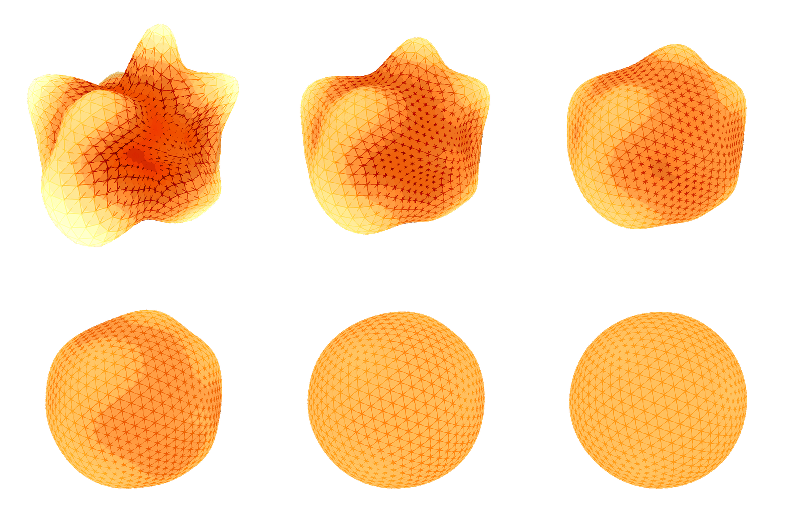
The idea of the heat method is based on the concept of heat diffusion. That is, given a surface \(S\) with a heat distribution function \(u_0\), the heat diffusion process is described by the heat equation:

\(\frac{\partial u}{\partial t} = \Delta u\)

where \(\Delta\) is the Laplace-Beltrami operator. As time goes by, the heat distribution function \(u\) will approach the steady state solution \(u_\infty\) where \(\frac{\partial u_\infty}{\partial t} = 0\).

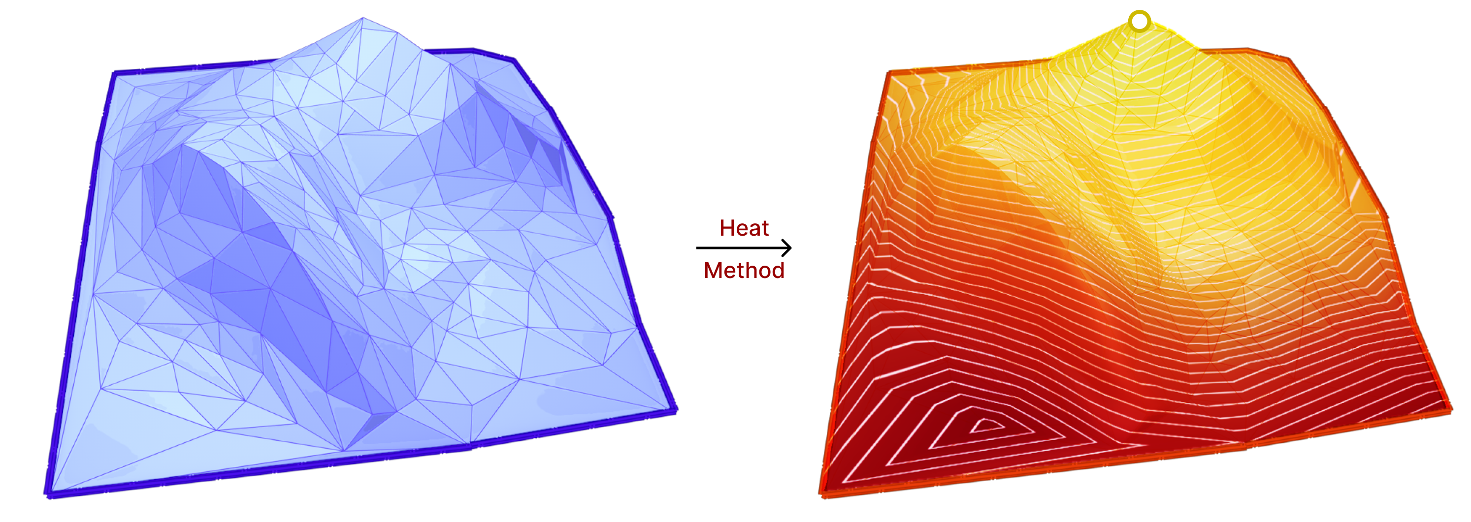
The heat method uses the heat diffusion process for a short period of time to compute the geodesic distance function. More specifically, the heat method consists of the following steps:

1. Initialize the heat distribution with heat source/s on surface vertices.
2. Let the heat diffuse for a short period of time. This involves solving the heat equation: \(\frac{\partial u}{\partial t} = \Delta u\).
3. Compute the gradient of the heat distribution function \(X = \nabla u\).
4. Normalize the gradient \(X\).
5. Finally, solve a simple Poisson equation to obtain the geodesic distance function \(\phi\).

\(\Delta \phi = \nabla \cdot X\)

From the above steps, we can see that the Laplace-Beltrami operator is used multiple times. Hence, this method is a good candidate to test the effects of our work on its accuracy. For more details on the heat method, we refer to “The Heat Method for Distance Computation“[15].

5.6.3 Evaluation Metrics

For evaluating the accuracy of the heat method, we use the exact polyhedral distance [16] function as a metric for comparison. The exact polyhedral distance metric provides the exact distance between two points on a polyhedral surface. Of course, the polyhedral mesh is an approximation of the original surface, so the exact polyhedral distance is not the same as the geodesic distance on the original surface. However, the exact polyhedral distance is a good enough approximation and it quickly gets closer to the geodesic distance of the original surface as the mesh resolution increases (quadratic convergence).

5.6.4 Benchmark Results

with the filtered Thingi10k meshes as a dataset, the exact polyhedral distance as a metric, the heat method was evaluated with mollification. We ran both of the algorithms with a random vertex as the source. We ran the benchmarks with different \(\delta\) values \(10^{-4}\) and \(10^{-2}\), scaled by the average edge length of the mesh. The results are summarized below:

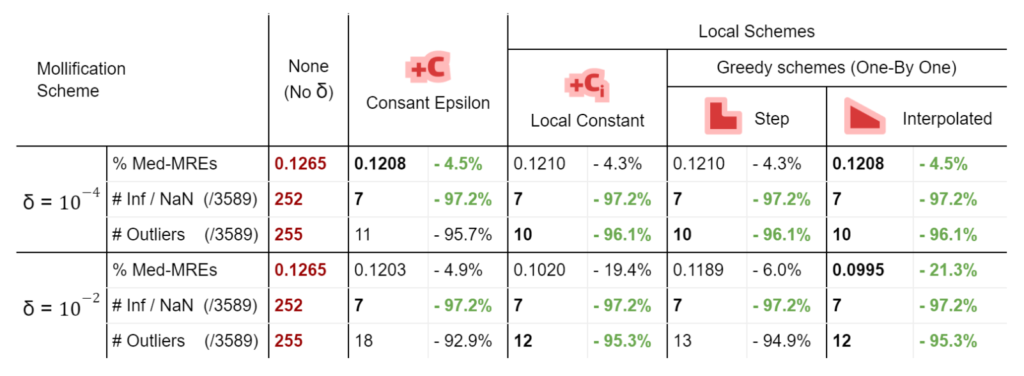
To measure accuracy, we computed the error as the Mean Relative Error (MRE) between the polyhedral distance and the heat method’s distance for each mesh. Since we are doing Single Source Geodesic Distance (SSGD), this is the mean of relative errors for all vertex distances from the source. We report the median of such MREs (Med-MREs) as a measure of how well each algorithm does on the whole filtered dataset (more than 3500 meshes).

There is an immediate improvement in accuracy using any Mollification algorithm in comparison to applying the heat method without any. In particular, for \(\delta = 10^{-4}\), we can see about \(~ 4.5\%\) of similar improvement for all schemes compared to no-mollification. This is true as well for smaller values like \(10^{-5}\) and \(10^{-6}\).

For large delta values (\(\delta = 10^{-2}\)), we can see that the local schemes produce significantly better results than the constant scheme (and no-mollification); Reaching an improvement of (~\(21.3\%\)) for the Median of MREs on the One-By-One Interpolated Scheme.

An important note is that we ran benchmarks multiple times with slightly different configurations. In some cases, the One-By-One Step scheme did better than the Local Constant One. But it was almost always the case that One-By-One Interpolated Scheme was a bit better than others for large \(\delta\).

In addition to MRE, we count the number of times the heat method produces infinity or NaN values (which is an indication of failure) as #inf | NaN. We also count the number of times where \(MRE > 100\%\). This is reported as #Outliers. It also includes in its count the times infinity or NaN values were produced.

Here is where Intrinsic Mollification truly shines; running the heat method implementation on the dataset directly results in about \(~ 252 / 3589\) failing cases (Infinities or NaNs). But, with the slightest mollification, 97% of these cases work fine. This is true for smaller values of \(\delta\) that aren’t shown in the table too (like \(10^{-6}\)). As for outliers, we notice that the Local Mollification algorithms tend to produce fewer outliers on average than the Constant Mollification scheme, especially when \(\delta\) is larger. The images below show some examples of the Outliers.

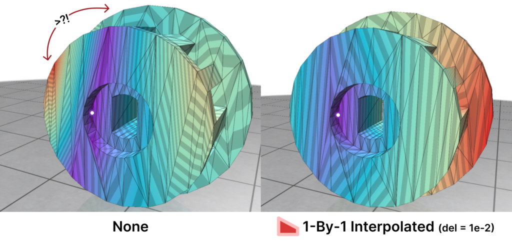
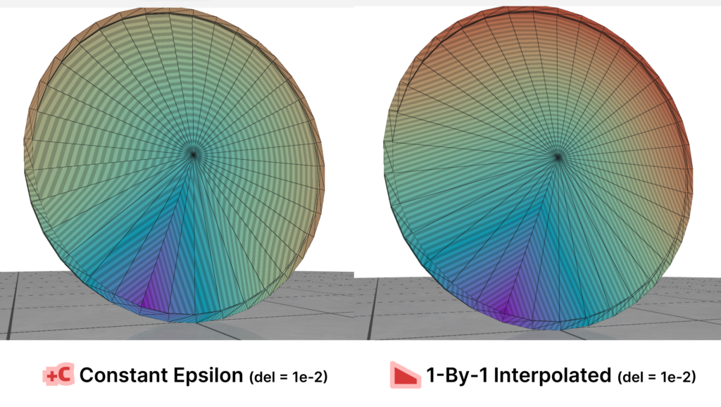
We ran this with and without the total length normalization step mentioned in 4.7. it had almost no effect on most of the mollification schemes. It is also interesting to see the behavior of each Mollification scheme with different $latex\delta$ values. Is there a best value for this parameter? The graph below shows this.

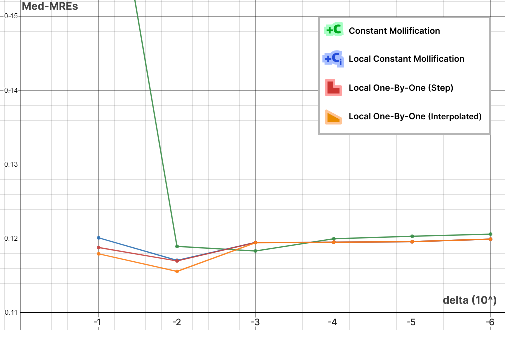
At least for the Heat method, one realization is that the local schemes allow higher \(\delta\) values than the constant scheme before the results get unreasonable. This is most likely because the local schemes mollify only where it is needed and with much less length distortion overall. Another realization is that \(10^-3\) and \(10^-2\) seem like optimal \(\delta\) values for the constant and local schemes respectively. We ran this benchmark a few different runs and with slightly different configurations but this fact seemed to hold for most runs.

As explained in the following section, we only ran this benchmark on the schemes shown in the table. It might be interesting to see how the others perform on the heat method. Also, we only ran these algorithms on meshes with atmost 20,000 faces to speed up the benchmark.

5.7 Notes on Implementation

we want to talk a bit about the benchmarks and the implementations of the heat method. we had trouble running/implementing it with Python and Libigl, so we switched to C++ and CGAL. We also had to rewrite the mollification algorithms in C++. Due to time constraints, we only managed to implement: the Constant, Local Constant, and Local 1-By-1 schemes. we think it would be interesting to try the other ones on the heat method and see their effects.

For the mollification schemes that use Linear or Quadratic programming, we used different solvers (SciPy and CvxOpt respectively). This makes the performance comparison between them questionable. Moreover, there might be other more time-efficient solvers. It would be interesting if that would increase the performance significantly.

6. Conclusions, Limitations, and Future Work

6.1 Conclusions

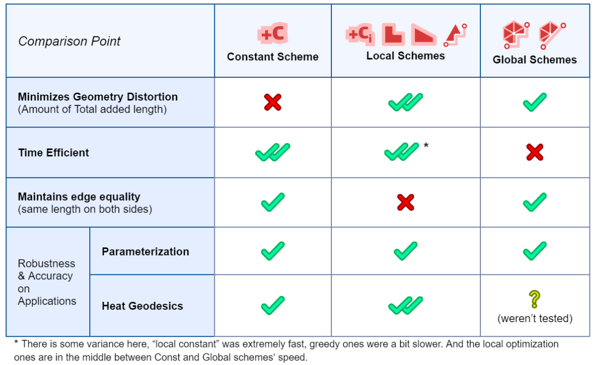
Based on all benchmarks applied, it is clear that Intrinsic mollification can make algorithms using the Cotan-Laplace matrix much more robust, especially against extremely skinny triangles. Moreover, it seems that the simple “bad-value” replacement hacks are not as effective.

As for comparing the newly introduced Mollification schemes with the original one, They aim to reduce the amount of added length, and succeed remarkably at that, decreasing the distortion in geometry greatly. This is an important result; because some applications and algorithms might require harder guarantees on (intrinsic) triangle quality. Thus, a higher \(\delta\) value can be used to achieve that without distorting triangles that are already in good shape.

Some of the Introduced schemes are global and highly time-expensive. However, the local schemes are reasonably fast and reduce added length most effectively among all mollification schemes.

Running these on the parameterization algorithms, all these schemes do not make any improvements over the constant scheme. On the other hand, It is true that on some algorithms (like the heat method), the local schemes do improve things quite remarkably.

6.2 Limitations

Intrinsic Mollification is a good pre-processing step because it is very simple and fast. But this is also the reason it is very limited; In particular, there’s only so much improvement you can hope to get by just changing edge lengths. For instance, if you don’t have enough resolution in one part of the mesh (or you have too much resolution), mollification won’t help.

there is also a trade-off between (intrinsically) better triangles and distorting the geometry too much. A simple example is having a cone vertex with very high valence which would get very distorted as shown below.

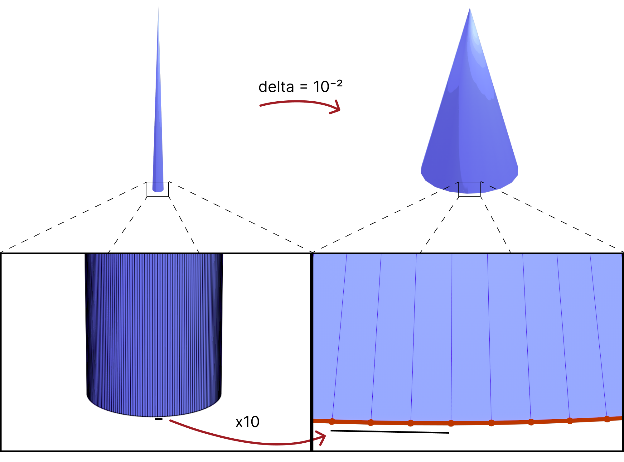
Lastly, In order to greatly reduce the amount of added length and only do that where it is needed, the local schemes sacrifice having the same edge length on both sides of the same edge. The Global schemes we worked on to solve this were either very slow (Linear/Quadratic programs over the whole mesh), or do not converge (sequential pooling schemes). So there is not one clear option that is fast, reliable, does not distort the geometry too much, and keeps edge lengths unbroken. However, that last property does not seem to practically affect the performance. So, some of the local schemes seem to be a favorable choice for a lot of applications.

6.3 Future Work

The work on this project was done in a very short period of time. So, we were not able to explore all the ideas we thought were promising. For example, If we find pooling operations that guarantee the Sequential Pooling schemes converge, then they can be much better alternatives than the global optimization schemes since those are very slow. Moreover, we would get a wide range of variants as we can use any of the local schemes as steps before each pooling iteration. We might even be able to compose such operations in interesting ways.

In this project, we only explored the effects of Mollification on the Laplacian. But it might be useful to apply Mollification before other types of computations where skinny and near-degenerate triangles harm robustness and accuracy and see if Mollification is effective in such cases.

the idea of Intrinsic Mollification is fresh and very flexible. Local schemes even reduce restrictions on the usage of this concept. Hence, we can try to find other usages (and formulations) than fixing skinny triangles. One example is “Intrinsic Delaunay Mollification”. Where we would consider the neighborhood of each edge, (locally) Mollify the 5 involved edge lengths so that the Delaunay condition is satisfied with the least amount of added length. In that case, each edge would have different lengths, but each one would be used in the appropriate iteration of edges around it. The figure below shows a sketch of this idea.

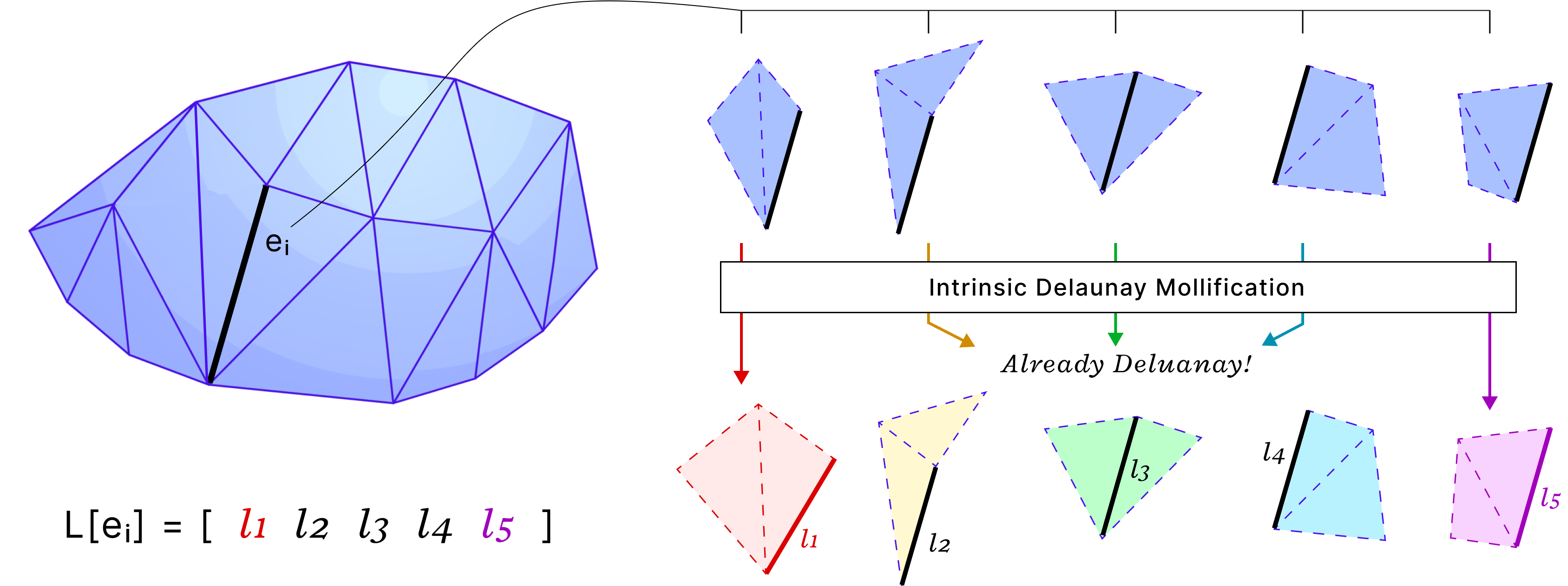
For the Local schemes, it might be worth trying to optimize their time performance by vectorized operations or parallelization. They are relatively fast, but there is some room for optimization there.

As mentioned in 4.7, normalizing to keep some properties unchanged may be a good idea to maintain certain aspects of the shape. Implementing the right normalization operation for the application might indeed be rewarding. One example to try is maintaining the same total area.

One of the most promising ideas is to try to apply this concept to Tetrahedral meshes. Tetrahedral meshes are often used in simulations, material analysis and deformations. These computations can behave poorly with bad-quality tetrahedrons. So, it is a great opportunity to apply the same concepts to this representation. Here, the problem is no longer just linear inequalities, but now we also have a nonlinear determinant condition (Cayley–Menger determinant). Nonetheless, it is a very interesting direction to put some effort into.

References

[1] Sharp Nicholas and Crane Keenan. 2020. A laplacian for nonmanifold triangle meshes. In Computer Graphics Forum, Vol. 39. Wiley Online Library, 69–80.

[2] Jonathan Richard Shewchuk. What Is a Good Linear Finite Element? Interpolation, Conditioning, Anisotropy, and Quality Measures, unpublished preprint, 2002.

[3] Khan, Dawar & Plopski, Alexander & Fujimoto, Yuichiro & Kanbara, Masayuki & Jabeen, Gul & Zhang, Yongjie & Zhang, Xiaopeng & Kato, Hirokazu. (2020). Surface Remeshing: A Systematic Literature Review of Methods and Research Directions. IEEE Transactions on Visualization and Computer Graphics. PP. 1-1. 10.1109/TVCG.2020.3016645.

[4] Fisher, M., Springborn, B., Schröder, P. et al. An algorithm for the construction of intrinsic Delaunay triangulations with applications to digital geometry processing. Computing 81, 199–213 (2007).

[5] Nicholas Sharp, Yousuf Soliman, and Keenan Crane. 2019. Navigating intrinsic triangulations. ACM Trans. Graph. 38, 4, Article 55 (August 2019).

[6] N Sharp, M Gillespie, K Crane. Geometry Processing with Intrinsic Triangulations. SIGGRAPH’21: ACM SIGGRAPH 2021 Courses.

[7] K Crane. 2018. Discrete differential geometry: An applied introduction. Notices of the AMS, Communication 1153.

[8] Zhou, Qingnan and Jacobson, Alec. “Thingi10K: A Dataset of 10,000 3D-Printing Models.” arXiv preprint arXiv:1605.04797 (2016).

[9] Georgia Shay, Justin Solomon, and Oded Stein. A dataset and benchmark for mesh parameterization, 2022., Vol. 1, No. 1, Article. Publication date: October 2023.

[10] Ligang Liu, Chunyang Ye, Ruiqi Ni, and Xiao-Ming Fu. Progressive parameterizations. ACM Trans. Graph., 37(4), jul
2018.

[11] Michael Kazhdan, Jake Solomon, & Mirela Ben-Chen. (2012). Can Mean-Curvature Flow Be Made Non-Singular?.

[12] Bruno Lévy, Sylvain Petitjean, Nicolas Ray, and Jérome Maillot. Least squares conformal maps for automatic texture
atlas generation. ACM Trans. Graph., page 362–371, jul 2002.

[13] Mullen, P., Tong, Y., Alliez, P., & Desbrun, M. (2008, July). Spectral conformal parameterization. In Computer Graphics Forum (Vol. 27, No. 5, pp. 1487-1494). Oxford, UK: Blackwell Publishing Ltd.

[14] Keenan Crane, Marco Livesu, Enrico Puppo, & Yipeng Qin. (2020). A Survey of Algorithms for Geodesic Paths and Distances. arXiv preprint arXiv:2007.10430

[15] Crane, K., Weischedel, C., & Wardetzky, M. (2017). The Heat Method for Distance Computation. Commun. ACM, 60(11), 90–99.

[16] Mitchell, J., Mount, D., & Papadimitriou, C. (1987). The Discrete Geodesic Problem. SIAM Journal on Computing, 16(4), 647-668.