Tag: SGI project

Intrinsic Mollification

Fellows: Hossam Saeed, Ikaro Costa, Ricardo Gloria, Sana Arastehfar

Mentored By: Keenan Crane

Volunteer: Zachary Ferguson

1. Introduction

Algorithms on meshes often require some assumptions on the geometry and connectivity of the input. This can go from simple requirements like Manifoldness to more restrictive bounds like a threshold on minimum triangle angles. However, meshes in practice can have arbitrarily bad geometry. Hence, many strategies have been proposed to deal with bad meshes (see Section 2). Many of these are quite complicated, computationally expensive, or alter the input significantly. We focus on a simple, very fast strategy that improves robustness immediately for many applications, without changing connectivity or requiring sophisticated processing.

Fig. 1. By intrinsically modifying edge lengths, we can get better Cotan Laplace weights for skinny triangles in the input mesh, making algorithms using the Laplacian more robust and accurate.

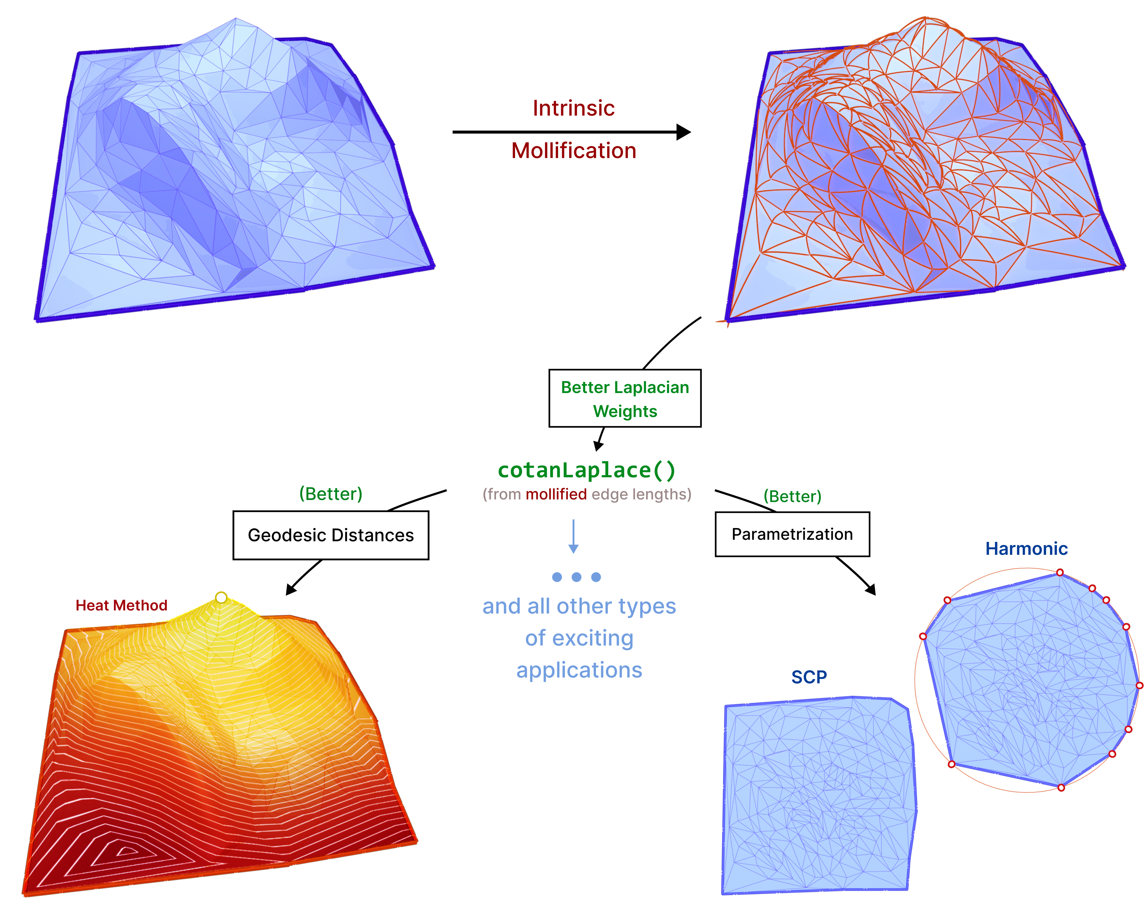
The main idea is that we can compute geometric quantities (like the Laplacian Δ) from an intrinsic representation (using edge lengths), This makes it easy to manipulate these lengths without moving vertices around, to improve triangle quality, and subsequently these computations. We introduce new schemes based on the same concept and test them on common applications like parameterization and geodesic distance computation.

Throughout this project, we mainly used Python and Libigl as well as C++, Geometry Central and CGAL for some parts.

1.1 What can go wrong?

When using the traditional formula to compute The Discrete Laplacian, many issues can arise. There are important challenges with the mesh that can harm this computation:

The mesh might not correctly encode the geometry of the shape.
Floating point errors: Inaccuracy and NaN outputs.
Mesh connectivity: non-manifold vertex and non-manifold edges.
Low-quality elements: like skinny triangles.

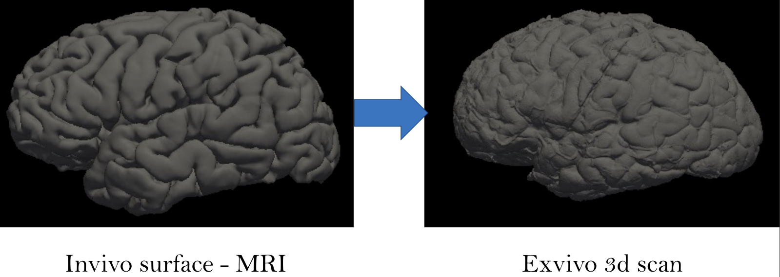
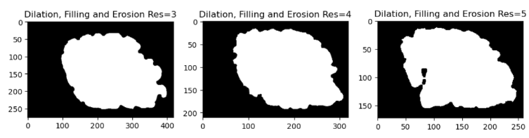
It is worth mentioning that (3) is addressed successfully in “A Laplacian for Nonmanifold Triangle Meshes” [1]. Throughout this project, we get deep into the challenge (4). Such elements can originate from bad scans, bad triangulations of CAD models, or as a result of preprocessing algorithms like hole-filling. A thorough analysis of bad-quality elements can be found in “What Is a Good Linear Finite Element?” [2].

Usually, to compute the Discrete Laplacian for triangular meshes, one uses the cotangent value of angles of triangles in the mesh (see section 3.2). Recall that $\cot\theta = \cos\theta / \sin\theta$. Therefore, an element having angles near 0 or 180 degrees will cause numerical issues as $\sin(\theta)$ will be very small if $\theta$ is near zero or near $\pi$.

1.2 What is the basic approach?

The triangle inequality states that each edge length of the three is a positive number smaller than the sum of the other two. Low-quality elements, such as the ones in the figure above, barely satisfy one of the three required triangle inequalities. For instance, if a triangle has lengths $a, b$ and $c$ where the opposite angle of $c$ is very close to $\pi$, then $a+b$ will be barely greater than $c$.

In a nutshell, the simple approach is to make sure that each triangle of the mesh holds the triangle inequalities by a margin. This is, for each corner in the mesh we guarantee that $a+b>c+\delta$ for a given $\delta > 0$. To accomplish this in each corner, we add the smallest possible value $\varepsilon>0$ to all edges in the mesh such that $a+b>c+\delta$ is held for each corner.

1.3 Contributions

We introduce a variety of novel intrinsic mollification schemes, including local schemes that operate on each face independently and global schemes that formulate intrinsic mollification as a simple linear (or quadratic) programming problem.

We benchmark these approaches in comparison to the simple approach introduced in “A Laplacian for Nonmanifold Triangle Meshes” [1]. We run them as a preprocessing step on common algorithms that use the Cotan-Laplace matrix. This is to compare their effect in practice. Of course, this comparison also includes comparing the effects of no mollification, and simple hacks against these schemes, as well as the effects of different parameters. This is discussed in great detail in the Experiments & Evaluation section.

A large amount of work has been done on robust geometry processing and mesh repair. In particular, there have been a variety of approaches to dealing with skinny triangles. These include remeshing and refinement approaches, the development of intrinsic algorithms and formulations, and simple hacks used to avoid numerical errors.

Remeshing can significantly improve the quality of a mesh, but they are not always applicable. Naturally, they alter the underlying mesh considerably. Moreover, may not be able to preserve the original mesh topology. In addition, remeshing is often computationally expensive and may be overkill if the mesh is already of good quality except for a few bad triangles. On the other hand, Mesh refinement at least preserves the original vertices. However, it increases the number of elements significantly and is still expensive in many cases. A thorough discussion of Remeshing algorithms can be found in “Surface Remeshing: A Systematic Literature Review of Methods and Research Directions” [3].

Fig. 3. (from [5]) Intrinsic Delaunay Triangulations (middle) fix some of the near-degenerate triangles ($\theta \approx 0^o$). Intrinsic Delaunay Refinement (right) provides bounds on minimum angles at the cost of introducing more vertices.

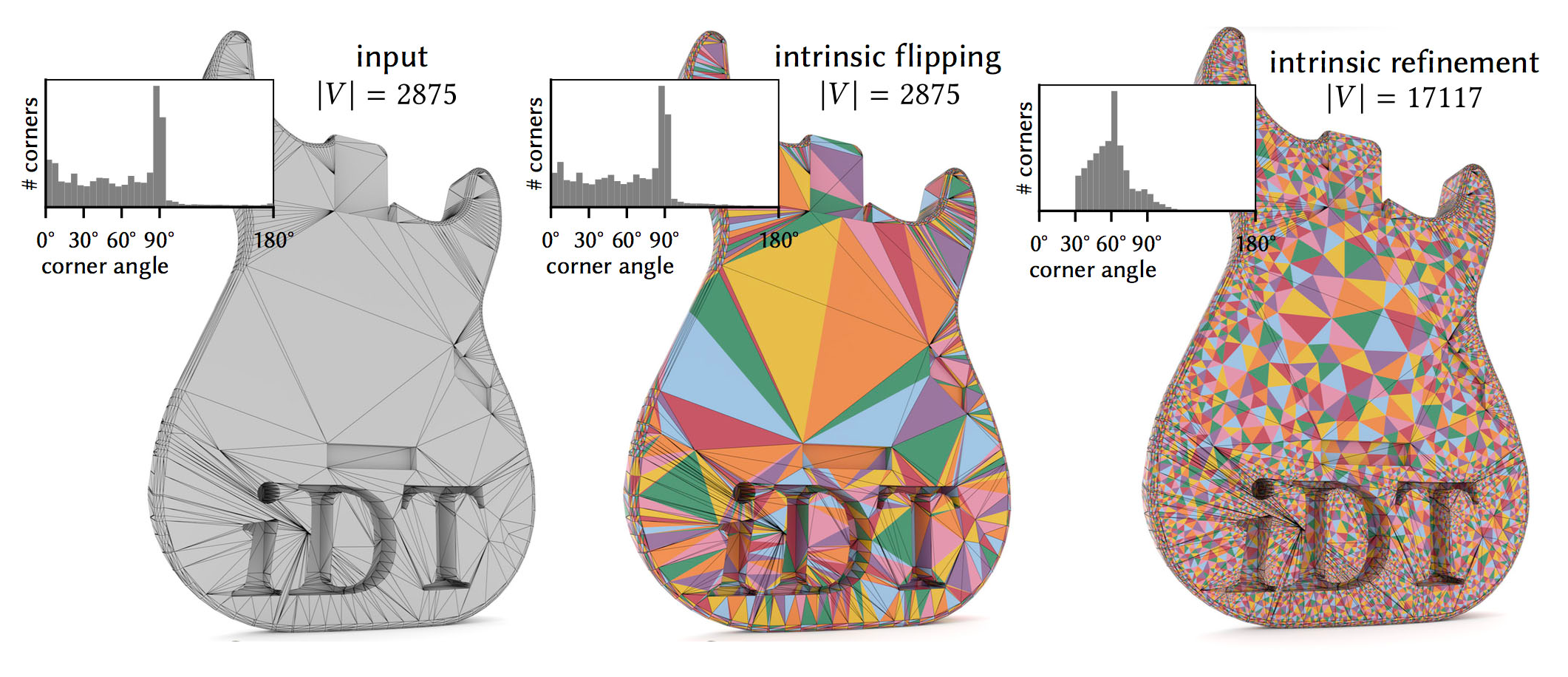
In contrast to extrinsic approaches that may damage some elements while trying to fix others, intrinsic approaches don’t need to move vertices around. For example, “Intrinsic Delaunay Triangulations” [4] using intrinsic flips can fix some cases of skinny triangles. However, it is not guaranteed to fix other cases. “Intrinsic Delaunay Refinement” [5] on the other hand provides bounds on minimum triangle angles at the cost of introducing more vertices to the intrinsic mesh. While these Intrinsic Delaunay schemes have many favorable properties compared to the traditional Remeshing and Refinement schemes, Intrinsic Mollification is much faster in case we only want to handle near-degenerate triangles. Moreover, it does not change the connectivity at all. For cases where an Intrinsic Delaunay Triangulation is required, we can still apply Intrinsic Mollification as a preprocessing step.

Lastly, Simple clamping hacks can sometimes improve the robustness of applications. But, they distort the geometry as they do not respect the shape of the elements corresponding to the clamped weights. Also, they seem to be less effective than mollification on the benchmarks we ran. They are discussed in detail in section 5.2.

3. Preliminaries

3.1 Intrinsic Triangulations

Our work is rooted in the concept of Intrinsic Triangulations. In practical Geometry Processing, triangular meshes are often represented by a list of vertex coordinates in addition to the connectivity information. However, we usually do not care about where a vertex is in space, but only about the shape of the triangles and how they are connected. So, working with vertex coordinates is not necessary and gives us information that can hinder robust computing.

Working with Intrinsic Triangulations, meshes are represented with edge lengths in addition to the usual connectivity information. In this way, we do not know where the object is, but we have all the information about the shape of the object. For a thorough introduction to Intrinsic Triangulations, see “Geometry Processing with Intrinsic Triangulations” [6] by Sharp et al.

3.2 Cotangent-Laplace Operator

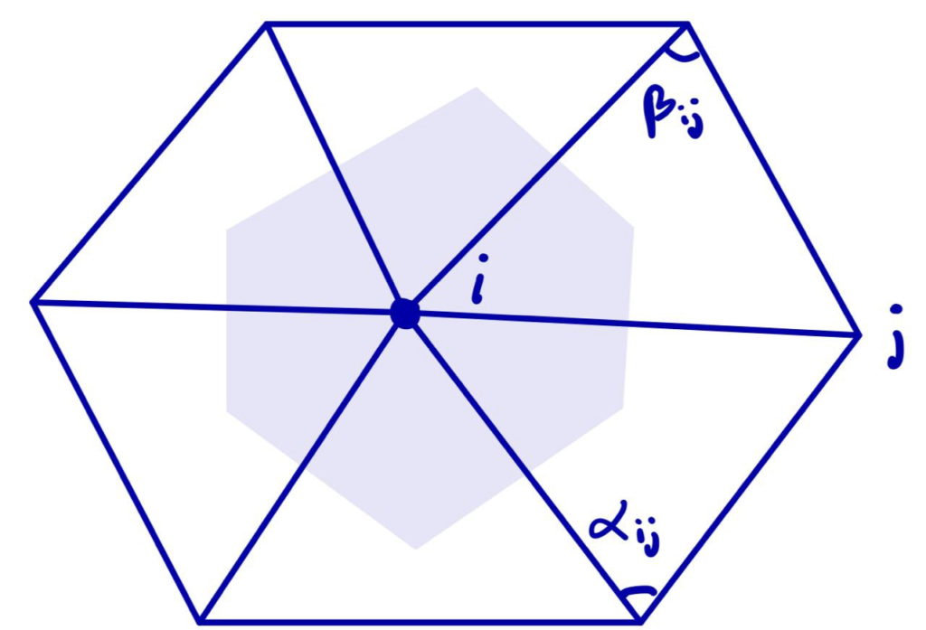
Recall that the Laplace operator $L$ acts on functions $f:M\to\mathbb{R}$ where $M$ is the set of vertices. For each vertex $i$ the cotangent-Laplace operator is defined to be

$(\Delta f)i = \frac{1}{2A_i}\sum_j (\cot(\alpha_{ij}) + \cot(\beta_{ij})(f_j – f_i)$

where the sum is over each $j$ such that $ij$ is an edge of the mesh, $\alpha_{ij}$ and $\beta_{ij}$ are the two opposite angles of edge $ij$, and $A_i$ is the vertex area of $i$ (shaded on the side figure).

The discrete Laplacian Operator is encoded in a $|V|\times |V|$ matrix $L$ such that the $i$-th entry of vector $Lf$ corresponds to $(\Delta f)_i$. The Discrete Laplacian is extremely common in Geometry Processing algorithms such as:

Shape Deformation.
Parameterization.
Shape Descriptors.
Interpolation weights.

4. Algorithm

Fig. 5. Intrinsic Mollification visualized on a mesh, The **blue** edges are the original (extrinsic) lengths, and the intrinsic (mollified) lengths are visualized as **orange** arcs that are longer while still having the same endpoints.

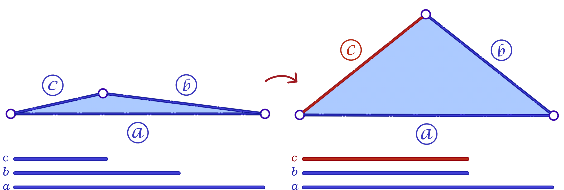
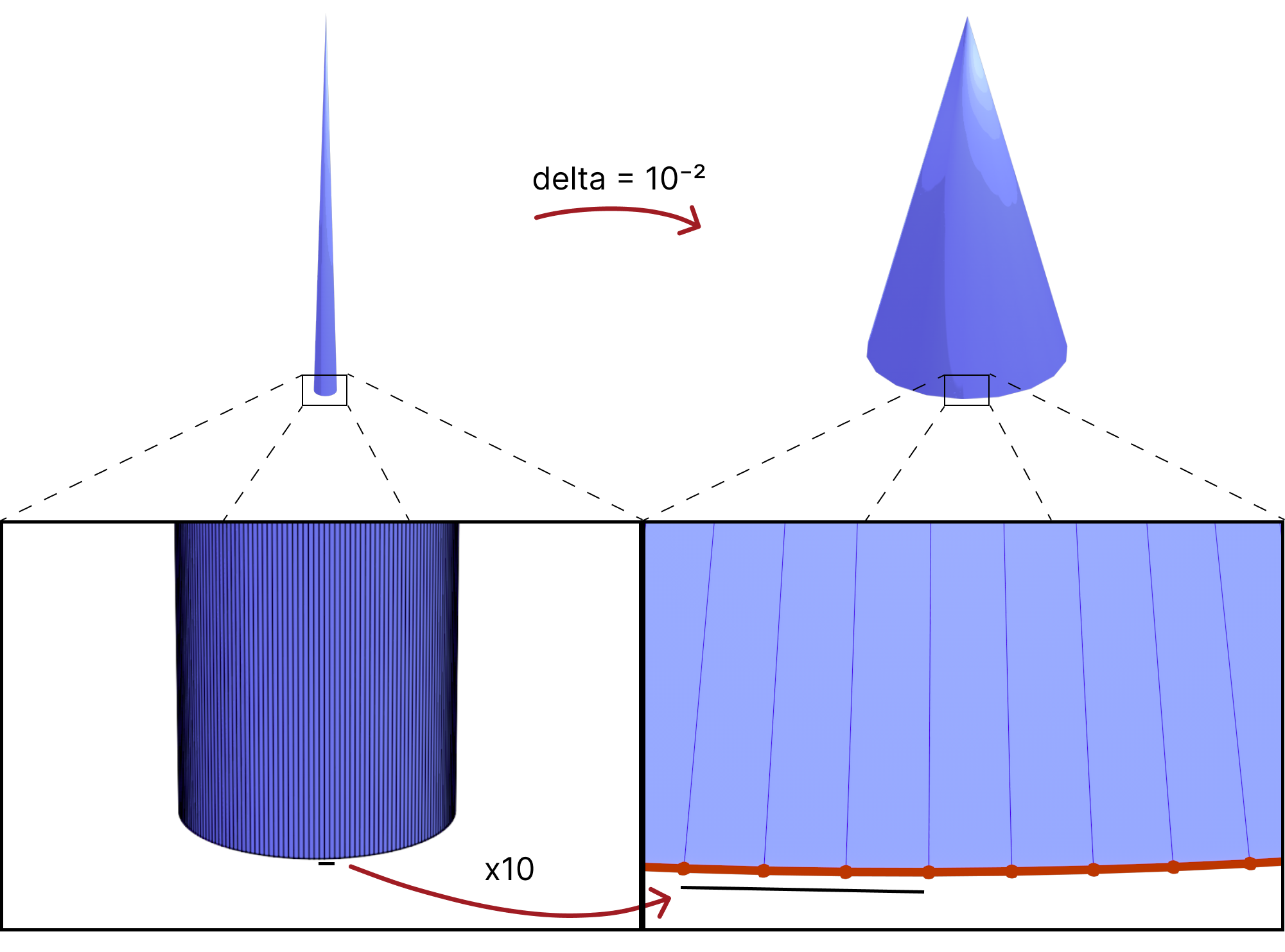
To solve the problem of low-quality triangles, we mollify each triangle in the mesh. By “mollify”, we mean pretending that the mesh has better edge lengths so that there are no (intrinsically) thin triangles in the mesh. Generally, for a mesh, equilateral triangles are the best to work with. If we add a positive $\varepsilon$ value to each of the edges of a triangle, the resulting triangle will be slightly closer to an equilateral one. In fact, it will become more equilateral as $\varepsilon$ approaches $\infty$. However, we don’t want to distort the mesh too much. So, we find the smallest $\varepsilon\geq 0$ such that by adding $\varepsilon$ to each edge of the mesh we end up with no low-quality triangles. A good way to think about Intrinsic Mollification is to fix the position of each vertex of the mesh and let the edges grow to a desired length, as illustrated in Figure 5 above.

4.1 The Constant Mollification Strategy

We first recap the strategy proposed by Sharp and Crane [1]. If a triangle has lengths $a, b$, and $c$, the triangle inequality $a + b < c$ holds even for very low-quality triangles. In order to avoid them, that triangle inequality must hold by a margin. This is, we ask that

$a + b < c + \delta$

for some tolerance $\delta > 0$ defined by the user. Then the desired value of $\varepsilon$ is

$\varepsilon = \max_{ijk} \max(0, \delta + l_{jk} – l_{ij} – l_{ki} )$

where each $ijk$ represents the corner $j$ of the triangle formed by vertices $i, j, k$ and each $l_{ij}$ represents the length of edge $ij$.

Phase I of this project consisted of implementing this functionality. Given the original edge lengths $L$ and a positive value $\delta$. The function returns the computed $\varepsilon$ and matrix $newL$ with the updated edge lengths in the same form as $L$.

Fig 6. The mollification output for different values of $\epsilon$ and base edge length $c$. The **red** triangle drawn bottom left shows how the intrinsically mollified lengths would look extrinsically (as if the vertices were moved to match the lengths).

The animation above shows, for a triangle, how the mollification output changes with different $\epsilon$ values and different lengths for the shortest edge in the triangle ($c$ in this case). Moving forward, when comparing with other Mollification schemes, we may refer to the Original Mollification scheme as the Constant Mollification scheme.

4.2 Local Mollification

One may think that the Constant Mollification scheme is wasteful as it mollifies all mesh edges. Usually, the mesh has many fine triangles and only a few low-quality ones. Therefore, we thought it is worth investigating more involved ways to mollify the mesh.

Fig. 7. Mollifying one face can make another face skinny (**red**), becoming in need of (more) mollification too.

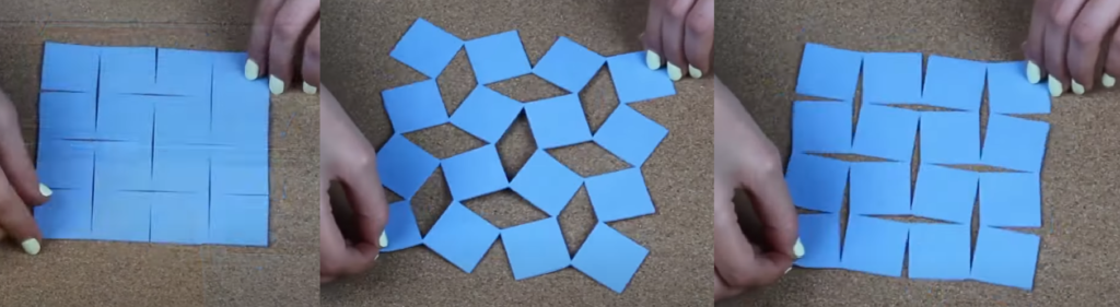
A naive approach is to go through all triangles and mollify only the skinny ones. However, while mollifying a triangle, the lengths of the adjacent triangles will change. Therefore, the triangles that were fine before may become violate the condition after mollifying the adjacent triangles. So, a naive loop over all triangles will not work, and it is not even clear that this approach will converge. The animation above shows a simple example of this case.

We had an idea to mollify each face independently. That is, we mollify each face as if it were the only face in the mesh. This breaks the assumption that the mollified length of any edge is equal on both sides of it (in its adjacent faces). The idea of having disconnected edges might be reminiscent of Discontinuous Galerkin methods and Crouzeix-Raviart basis functions.

Fig 8. By allowing the mollified edge length to be 2 different values for its 2 sides (halfedges), we can mollify each face independently from its neighbors.

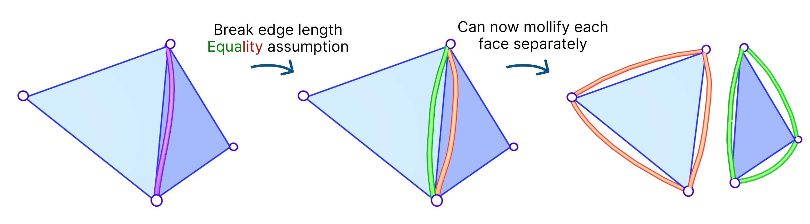
The algorithm for this approach is basically the same as the original one, except that we find $\varepsilon$ for each face independently. We call this approach the Local Constant Mollification scheme. Here, it might sound tempting to let $\delta$ vary across the mesh by scaling it with the local edge length average. However, this did not work well in our experiments.

It is reasonable to think that breaking edge equality might distort the geometry of the mesh, but it is not clear how much it does so compared to other schemes as they all introduce some distortion including the Constant Mollification one. This is discussed in the section 5.3.

4.3 Local One-By-One Mollification

Fig. 9. The Greedy Mollification Process. The smallest edge ($c$) is mollified till the needed $\delta$ is satisfied, the other edges might also be mollified to make sure $c \le b \le a$ holds.

Since we are considering each face independently, we now have more flexibility in choosing the mollified edge lengths. For a triangle with edge lengths $c \le b \le a$, one simple idea is to start with the smallest length $c$ in the face and mollify it to a length that satisfies the inequalities described in the original scheme. To mollify $c$, we simply need to satisfy:

$c + b \ge a + \delta \quad\text{and}\quad c + a \ge b + \delta$

After mollifying $c$, it is easy to prove that we only need to keep $a \ge b \ge c$ for the third inequality to hold. This scheme can be summarized in the following 3 lines of code:

c = max(c, b + delta - a, a + delta - b)
b = max(b, c)
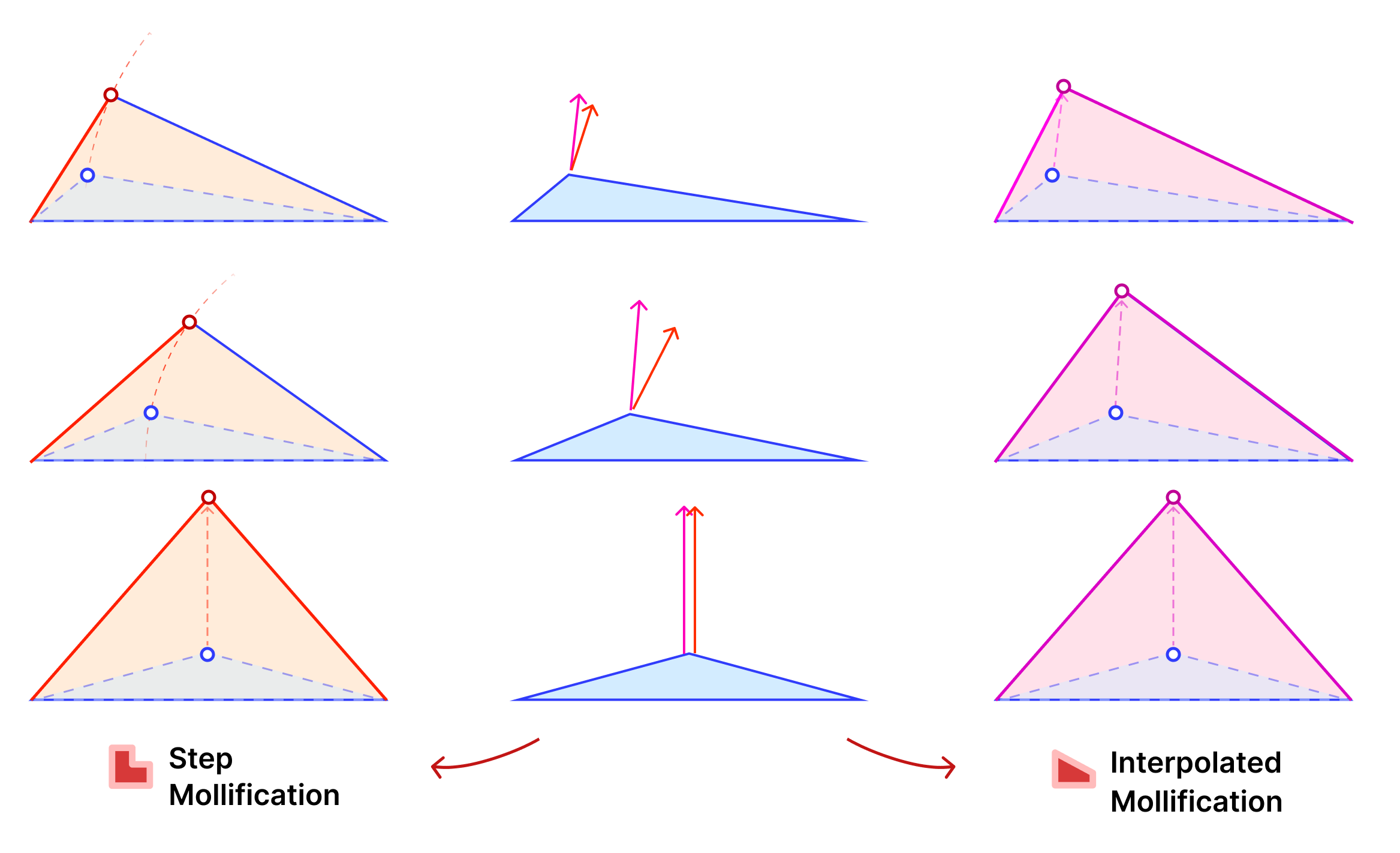
a = max(a, b)

The animation in Figure 9 above visualizes this process. We call this approach the Local One-By-One (Step) Mollification scheme.

A slight variation of this scheme is to mollify $b$ along with $c$ to keep differences between edge lengths similar to the original mesh; this is to try to avoid distorting the shape of a given triangle too much (of course we still want to make skinny triangles less skinny). Consider the following example. Suppose the mollified $c$ equals the original length of $b$. If $b$ isn’t mollified, we would get an isosceles triangle with two edges of length $b$. This is a big change to the original shape of the triangle as shown below. So a small mollification of $b$ even for smaller “$\delta$”s might be a good idea.

Fig. 10. Due to its discontinuous nature, the simple (step) version might change the shape of a triangle, making a (clearly) Scalene triangle an Isosceles one.

But how much should we mollify $b$? To keep it at the same relative distance from $a$ and $c$, we can use linear interpolation. That is, if $c_o$ was mollified to $c_o + eps_c$. we can mollify $b_o$ to $b_o + eps_b$ where

$eps_b = eps_c * \frac{a_o – b_o}{a_o – c_o}$

We call this approach the Local One-By-One Interpolated Mollification scheme. It can be summarized in the following 4 lines:

c_o = c
c = max(c, b + delta - a, a + delta - b)
b = max(c, b + (c - c_o) * (a - b) / (a - c_o))
a = max(a, b)

One more advantage of this interpolation is that it makes the behavior of $b$ mollification smoother as $\delta$ changes; This is visualized by the animation below.

Fig. 11. Showing how the output of each of the 2 greedy versions changes as a function of 𝛿.

Another perspective on the behavior difference between both versions is to look at different cases of skinny triangles mollified with the same $\delta$ value. As shown below, the Interpolated version would try to lessen the distortion in shape to keep it from getting into an isosceles triangle very quickly. Thus, having more variance in the mollified triangles’ shapes.

Fig. 12. The 2 One-By-One versions applied on a variety of skinny triangles. the “Step” one gets to the isosceles case quickest, while the “Interpolated” one affects the ratios between edges much less.

A great property of both schemes over the constant ones is that $\delta$ does not need to go to ∞ in order to approach an equilateral configuration. In fact, we can prove that the mollified triangle is guaranteed to be equilateral if $\delta \ge {a – c}$.

4.4 Local Minimal Distance Mollification

Fig. 13. The coordinate space of triangle lengths, where each point represents a triangle (left). Mollification can be thought of as a vector from the original triangle to the resulting one (middle). By placing the original triangle at the origin, the coordinates of the mollified triangle represent the $\varepsilon$ values and are all in the first octant (right).

Even with the one-by-one schemes, We don’t have a guarantee that the triangle mollification is minimal. By minimal we mean that the mollified triangle is the closest triangle to the original triangle in terms of edge lengths. This is because greedy schemes don’t look back at the previous edge lengths and potentially reduce the mollification done on them.

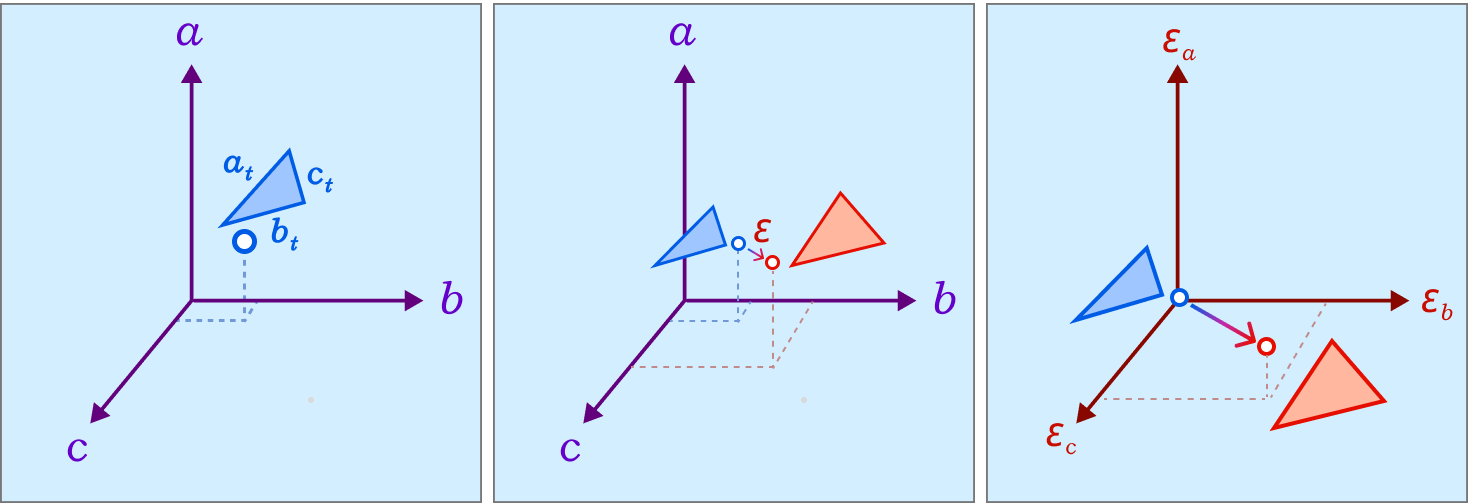
A good result from working with intrinsic lengths is that it is easy to deal with one triangle at once if we think about each edge as an independent variable. Then, the original triangle is a point in the space of edge lengths and the mollified triangle is another one. Since we are only adding length, it is easier to think of the original triangle as the origin point of this space and all vectors would represent the added length to each edge. Thus, the 3 axes now represent each edge’s $\epsilon$. This is illustrated in the Figure above.

The problem of finding the minimal mollified triangle is then a problem of finding the closest point to the original triangle in this space inside the region defined by 6 constraints (triangle inequalities & non-negativity of epsilon). These make up a 3D polytope as shown below.

Fig 14. The intersection of the 3 mollification inequalites results in a tetrahedral-like region independent of the specific triangle at hand (left). One triangle represents a point in the length space and the has 3 dependent ineuqallities (right) restricing mollification to positive $\varepsilon$. The 6 ineuqalities together make the constraint region.

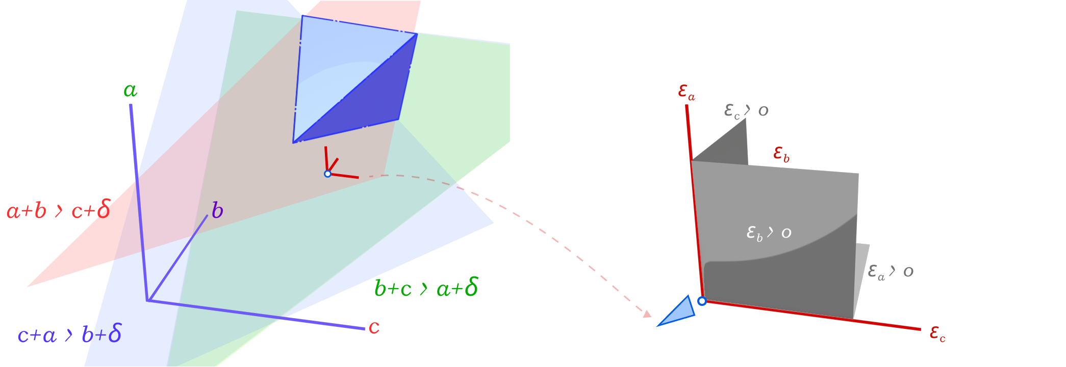
Depending on how we define the distance between two triangles, this problem can be solved using Linear Programming or Quadratic Programming. We can define the distance between two triangles as the sum of the distances between each corresponding edge of both triangles, this distance is just the $L_1$ norm (Manhattan) of the difference between the edge lengths of the two triangles. This is a linear function of the edge lengths. Therefore, the problem of finding the minimal mollified triangle is the following Linear Programming problem:

$\begin{gather*}
\text{min} \quad
I_{3 \times 1} \cdot x \\
\\
\text{s.t.} \quad
\begin{pmatrix} 1 & 1 & -1 \\ 1 & -1 & 1 \\ -1 & 1 & 1 \\ 1 & 0 & 0 \\ 0 & 1 & 0 \\ 0 & 0 & 1 \end{pmatrix} x =
\begin{pmatrix} \delta \\ \delta \\ \delta \\ 0 \\ 0 \\ 0 \end{pmatrix} \\ \end{gather*}$

The first 3 rows correspond to the 3 triangle inequalities, and the other 3 restrict mollification to positive additions to the length.

In the other case, where we define the distance between two triangles as the $L_2$ norm (Euclidean) of the difference between the edge lengths of the two triangles, the problem of finding the minimal mollified triangle is a Quadratic Programming problem. The constraints are still the same, the only difference is that we minimize $x^T x$ instead of $I_{3 \times 1} \cdot x$. The good news is that both problems can be solved efficiently using existing solvers. The figure above visualizes both concepts.

With these 2 versions, we have two more schemes, namely, the Local Minimal Manhattan Distance and the Local Minimal Euclidean Distance mollification schemes

4.5 Sequential Pooling Mollification

Fig. 15. The process of repeatedly mollifying and averaging (pooling) till convergance.

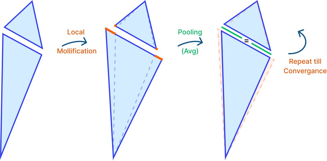
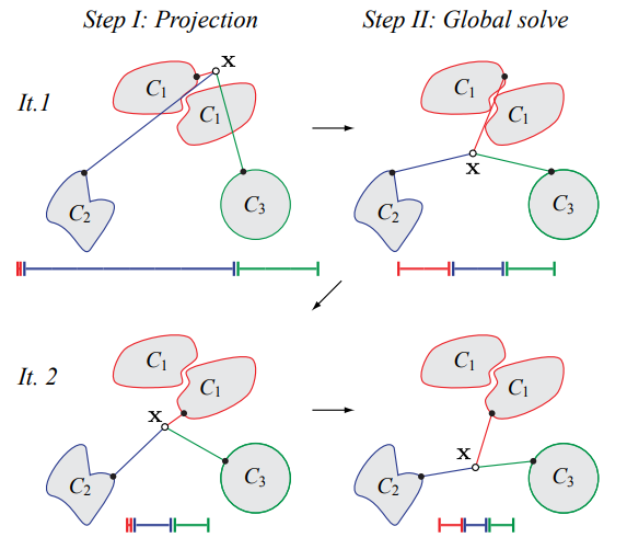
After exploring a lot of different local mollification schemes, we thought it would be a good idea to try to get the advantages of local mollification schemes (like significantly reducing the total mollification) while still keeping the edge lengths on both sides equal. The first idea that came to mind was to mollify the mesh using local scheme, and then average the mollified edge lengths on both sides of each edge. And repeating this process until convergence. The figure above visualizes this idea.

When we tried this idea on a few meshes, we noticed that the mollification process was not converging. We tried other pooling operations like Max, Min, and combinations of them. Unfortunately, none of them were converging. It might be worth it to put some time into trying to derive different pooling functions with convergence guarantees.

4.6 Global Optimization Mollification

In the search for a scheme that has a lot of the good properties of the local schemes, while keeping edge lengths on both sides equal, we took the idea of finding the closest mollified triangle to the original triangle in terms of edge lengths, but instead of doing it locally, we will apply the problem to all mesh edge lengths at once.

This also involves solving a Linear Programming or Quadratic Programming problem based on the distance function we choose. We call the global versions the Global Minimal Manhattan Distance and the Global Minimal Euclidean Distance Mollification. Effectively, this is finding the least amount of mollification while not breaking the equality of edge lengths on both sides.

4.7 Post-mollification Normalization

Since we are always adding length in mollification, Properties that aren’t scale invariant might get scaled. In order to avoid this, we might want to scale the mollified edge lengths down so that the total surface area is the same. This would not make a difference for the Cotan-Laplace Matrix but it can a difference for the Mass Matrix (among other things).

For some applications, it would make sense that we want a different quantity to remain unchanged after the mollification. For example, To keep the geodesic distances from getting scaled up, we can normalize the mollified edge lengths so that the total edge length is the same after mollification. for each mollified edge length $e^i_{mol}$:

$e^i_{mol}- = e^i_{mol} * \frac{\sum_{j = 1}^{|E|} e^j_{mol}}{\sum_{j = 1}^{|E|} e^j}$

We implemented this step in our C++ implementation and used it in the Geodesic Distance Benchmarks in.

5. Experiments and Evaluation

5.1 Data Sets for Benchmarks

Fig. 17. Thingi10K Filtered. Acceptable meshes can have arbitrary genera, number of connected components, and geometry. It is worth noting that this and other illustrations were inspired by Keenan’s work on his courses and in [7].

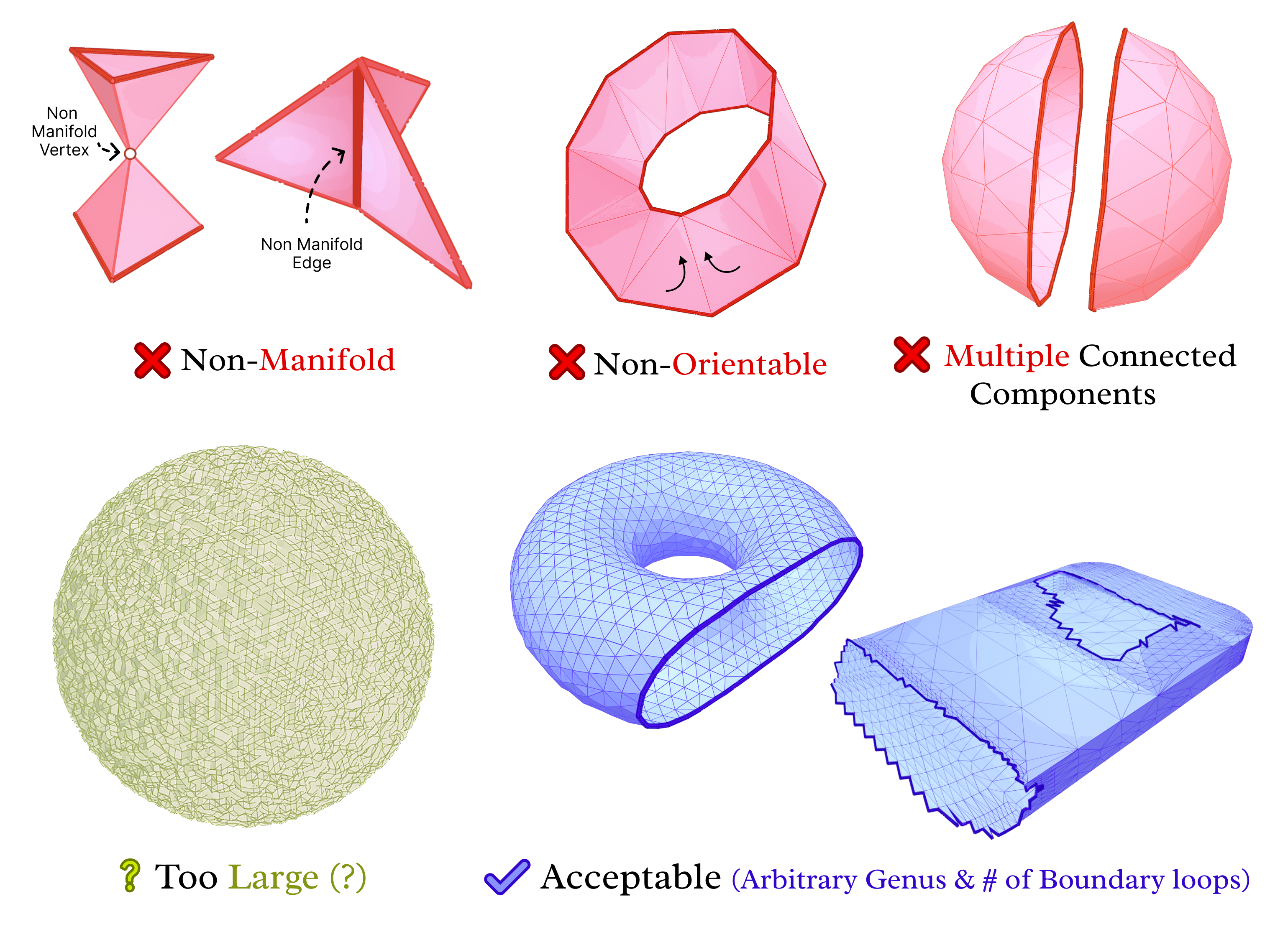
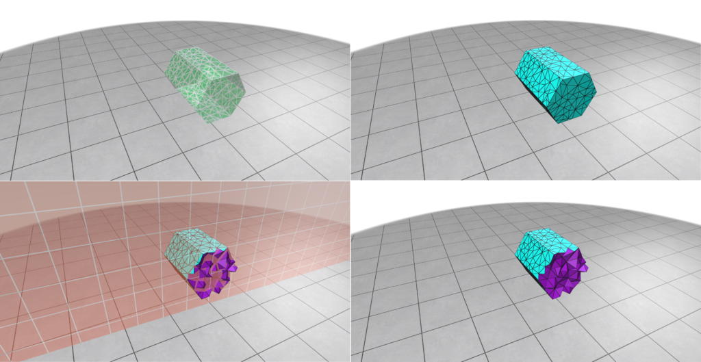
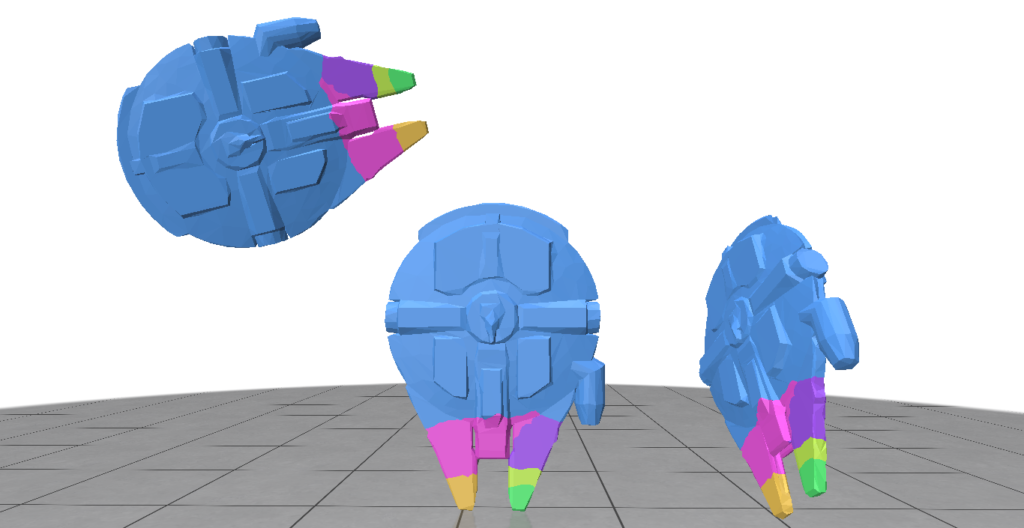
For most experiments, we use the Thingi10k data set [8]. It is composed of 10,000 3D models from the Thingiverse. The models have a wide variety of triangular meshes. This variety comes in regards to Manifoldness, genus, number of components and boundary loops, and more. A lot of the meshes also have very bad quality triangles. So, it is suitable for testing our work on a wide range of scenarios.

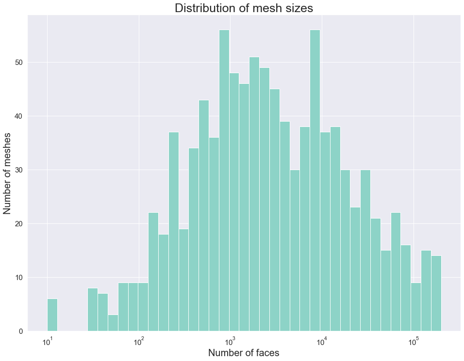
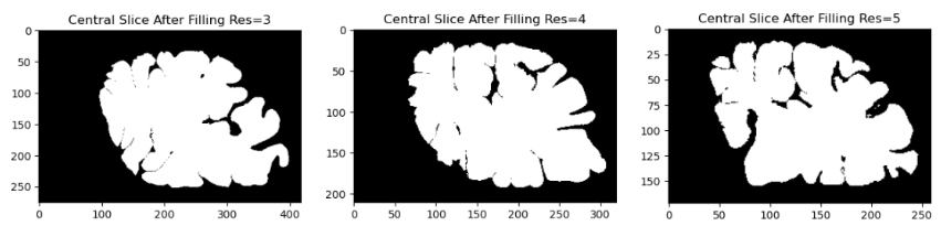
We implemented a script to filter the data set. In particular, we removed not manifold, multiple-component, and non-oriented meshes. The remaining meshes are categorized based on the size of the mesh and the number of skinny triangles (i.e. ones that violate the mollification inequalities). This step was very helpful for testing and debugging the different aspects of the proposed work quickly by choosing the appropriate meshes. The Figure above shows examples of acceptable and filtered-out meshes. For most of the benchmarks, we used this filtered data set . In some cases, we filtered out large meshes (i.e. $\|F\| > 20,000$ triangles) to reduce the running time of the experiments. The graph below shows the (log) distribution of the number of faces used for some of the benchmarks.

Fig 18. Filtered Thingi: a histogram of face counts. With a logarithmic x-scale, It seems very close to a log-normal distribution.

In search for other data sets to evaluate the proposed work, “A Dataset and Benchmark for Mesh Parameterization” [9] has an interesting set of triangular meshes used to benchmark parameterization schemes. As described, Thingi10k meshes come from real data, usually used for 3D printing and video game modeling but the data is not particularly suitable for testing parameterization methods. Since mollification will be important for parameterization methods, the investigation of further data sets is needed.

“Progressive parameterizations” [10] presents a data set which has been used before in the literature for benchmarking parameterization methods. However, [10] data is composed of meshes based on artificial objects. In this case, [9] obtain and makecorrection corrections on meshes from multiple sources, including the Thingiverse, which are mainly obtained from real-world objects and form the set called Uncut. Then, in possession of the Uncut, they perform cuts along the artist’s seam to form the set called Cut. . Due to time limits, The parameterization benchmarks currently reported are still on Thingi10k (with some work to extract patches). But, it may be worth it to use Cut for the parameterization benchmarks in the future.

5.2 Alternative Strategies

The effects of badly shaped triangles have been present since the early days of mesh generation. A common appearance of these effects is on Surface Parameterization Problems. Examples of these problems are the Least Squares Conformal Mapping and Spectral Conformal mapping, which essentially are composed of vertex transformations whose weights are in their essence non-negative. However, it is known that very thin triangles can result in parameterization weights that are negative or numerical zeros which need to be avoided.

In practice, simple heuristics have been applied to avoid non-positive conformal map weights. These are indeed simple in nature but known to be in some cases effective

Replace negative weights with zero, or with absolute value
Replace NaN & infinity weights with zero, or with one.
Replace numerical zeros with zero.

We tried using some of these hacks and even combinations of them. Hence, Some of them turn out to be more useful and produce better results. For example, for the parameterization benchmarks, the negative replacement hacks were not useful at all. On the other hand, the NaN (& Infinity) replacement hacks are much more useful. Also, the near-zero approximation hack improves things sometimes but makes things worse more often. Overall, it is not immediately clear if any of them are better in a general sense.

For this, given an appropriate measure to be discussed in the mapping benchmarks in section 5.5.4, the Mollification schemes are compared to the best-performing combinations of these simple heuristics.

5.3 Comparison of Mollification Strategies

5.3.1 Length Distortion

First, we compare all schemes’ performance independent of any application; to see how much they affect the mesh geometry. For each mesh in Thingi10k (filtered), we compute the relative total difference between the mollified and original lengths. These differences are averaged over all meshes and reported as Avg. Added Length as a metric of length distortion. We also report the average percentage of mollified edges (for global schemes, it can not be counted explicitly).

Table 1. Summarizing the effect of each Mollification scheme on the edge lengths on average.

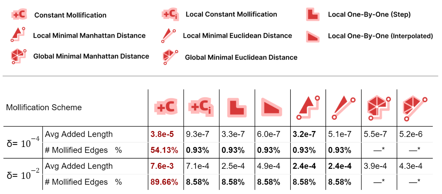
Local schemes introduce much less mollification than the constant one as they only mollify near-degenerate faces, especially for smaller $\delta$; due to having less strict inequalities and thus less faces violating them. The number of mollified edges is x50 times smaller for local schemes.

For the average added length, Unsurprisingly, The Local Minimal Manhattan distance scheme is always optimal. For the Euclidean distance version, it has more added length because the metric we are reporting is essentially a scaled sum of Manhattan distances for each face. Additionally, the Local 1-by-1 Step scheme is always very close to the Local Minimal Manhattan distance scheme as in most cases, we only need to mollify one edge. In such cases, Both schemes behave identically.

Compared to the step version, the Local 1-by-1 Interpolated scheme allows some more length distortion for smoother behavior over $\delta$ values and better triangle length ratio preservation. Moreover, this distortion is still quite low compared to the Local Constant scheme.

The Global Minimal distance schemes have significantly less added length than the constant one, and more than the local analouges. But, they have the benefit of keeping the 2 sides lengths of an edge equal. The Euclidean version has a strangely larger added length than the Manhattan one for $\delta = 10^{-4}$. This might be worth investigating further.

More than 50% of the dataset needs mollification even for forgiving $\delta$ values, which shows that skinny triangles are common in practice. This motivates the development of mollification and other preprocessing step.

5.3.2 Time Performance

It is important to also analyze the time performance of these schemes. The table below shows the average running times for the filtered dataset meshes with $\|F\| \le 200,000$.

Table 2. Showing the average running time for each scheme on the filter Thingi10k dataset.

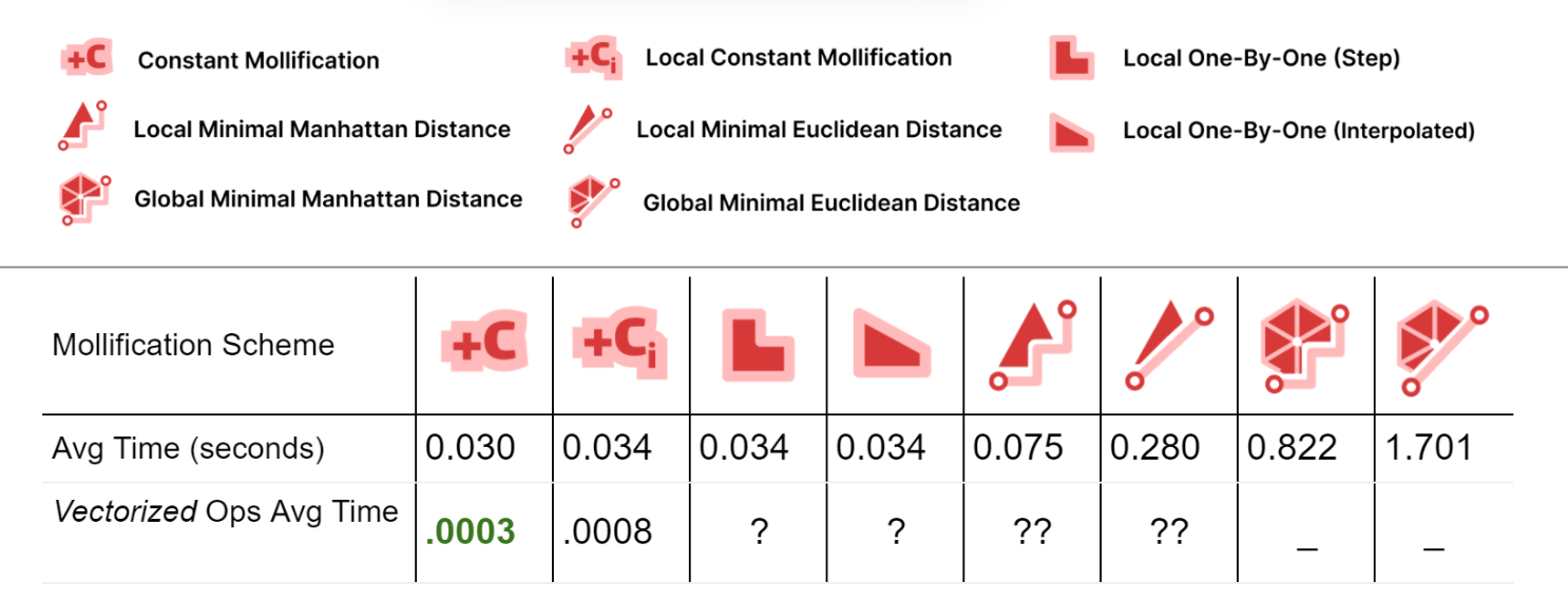
First, comparing the basic implementations (With no vectorized NumPy Operations), we see that most of the local schemes have very similar running times to the constant scheme (the fastest). This is great news because the extra steps implemented in them don’t have a large impact on the average running time.

For the Local Minimal distance schemes, they are a bit slower. But it is important to note here that we didn’t try to find the most efficient libraries for linear programming and quad programming optimizers; In fact, we used a different one for each problem (Scipy and Cvx-Opt respectively). So, for a more careful performance analysis, it would be worth trying different libraries and reviewing the implementation. It can also be beneficial to try to find a simple update rule form for them (similar to the implementation of the greedy ones). From the first glance, it sounds feasible, especially for the linear program version as it is extremely similar to the 1-by-1 step scheme.

For the global minimization schemes, they are much slower than the others. Here, the notes mentioned above about efficient optimizers also hold.

To improve the running times, we implemented the Constant scheme and the local Constant schemes using NumPy’s vectorized operations. It is clear that this made a huge difference (about x100 and x40). We didn’t have time to try to do the same for the other local schemes. But it might be achievable and it would be interesting the resulting boasts. Moreover, the local schemes are very easy to parallelize which is one more way to optimize them. Since the local schemes’ time is mostly spent iterating over the faces and checking them, they can be integrated into the Laplacian computation loop directly to save time.

Fig. 19. For each scheme, the graph shows how the mollification running times increase in relation to the number of faces of the mesh.

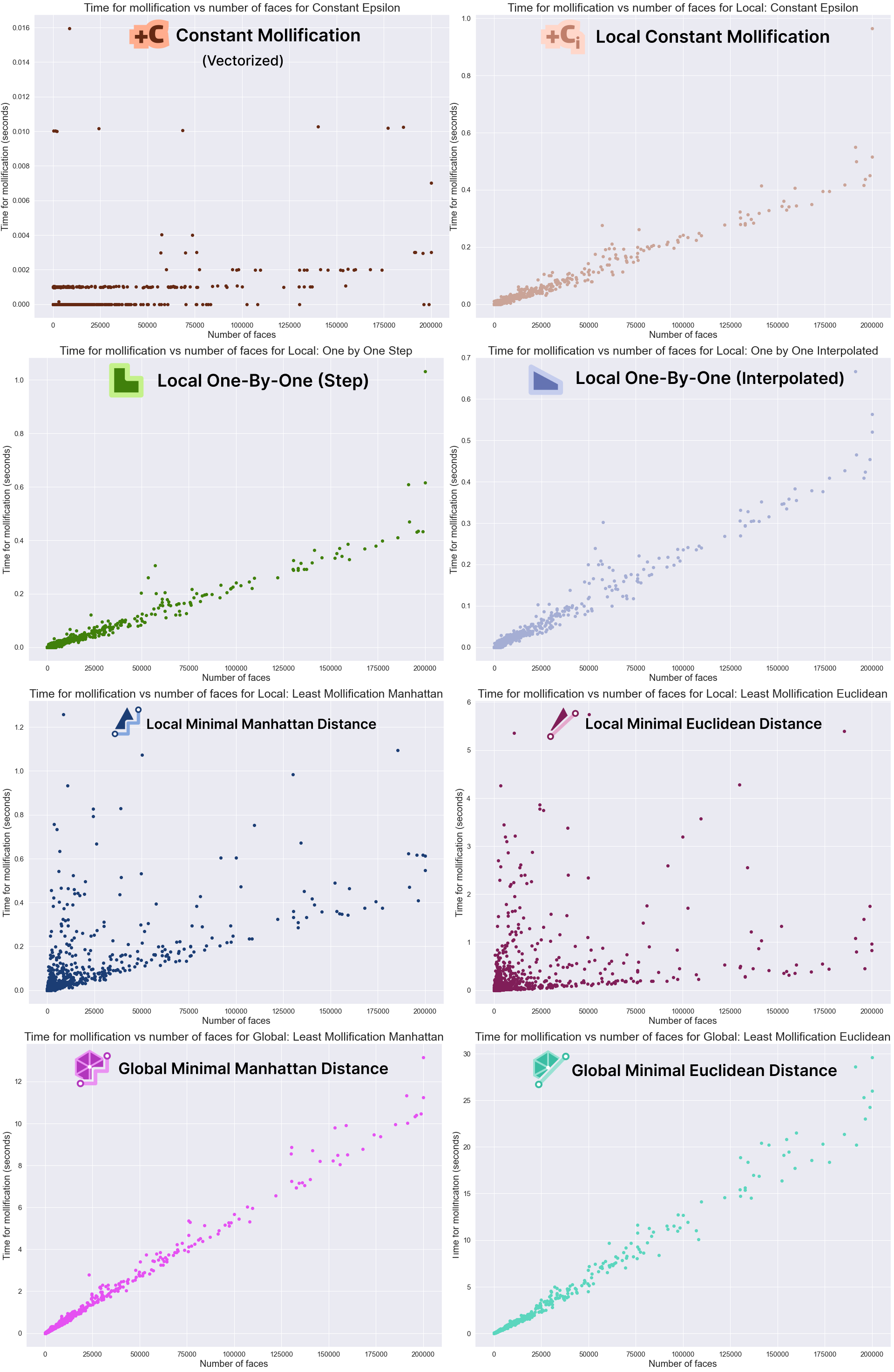
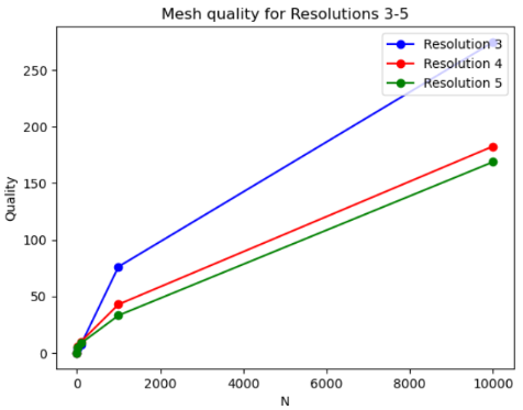
The graphs above show that the Mollification schemes have a linear running time in relation face counts. Indeed, this is obvious for the local schemes as each face is processed independently. The local minimal distance schemes uniquely have very high variance, it is not as clear why this happens, though. For the vectorized implementation of the constant scheme, the running time is too small to be able to draw a pattern. Finally, although the global schemes also have linear growth, they are too slow in comparison. For example, a mesh with about 200,000 faces would take about 10 seconds for the Manhattan version and 25 for the Euclidean distance version on average. It is not clear how much performance gain we would get from a more optimized implementation with more efficient libraries.

5.4 Mollification + Simple Applications

Fig. 20. Solving the Poisson equation on a density function over mesh vertices.

Fig. 21. An animation showing the mean curvature flow over the bunny mesh with different time step values.

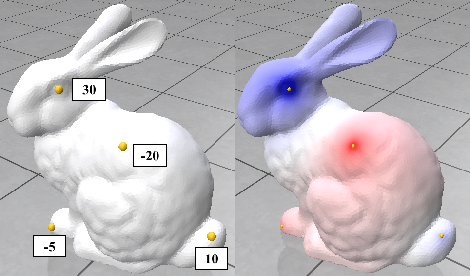
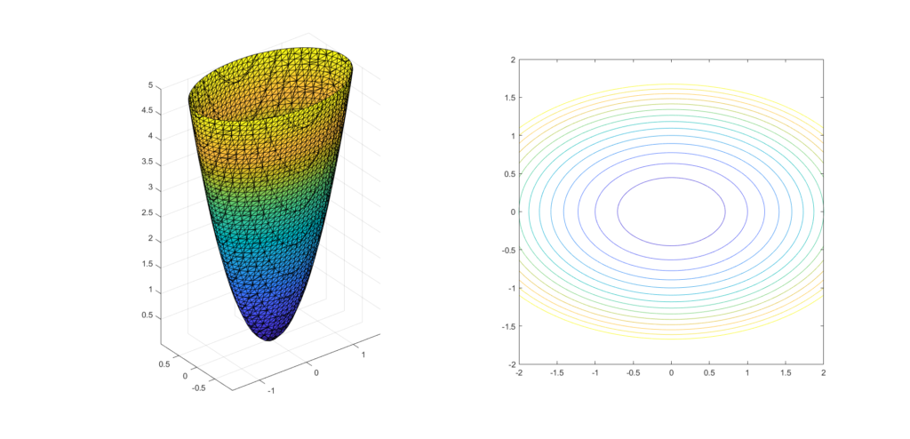
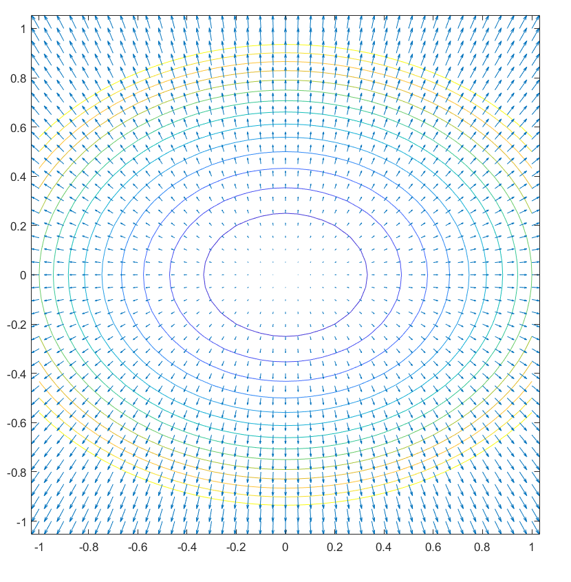
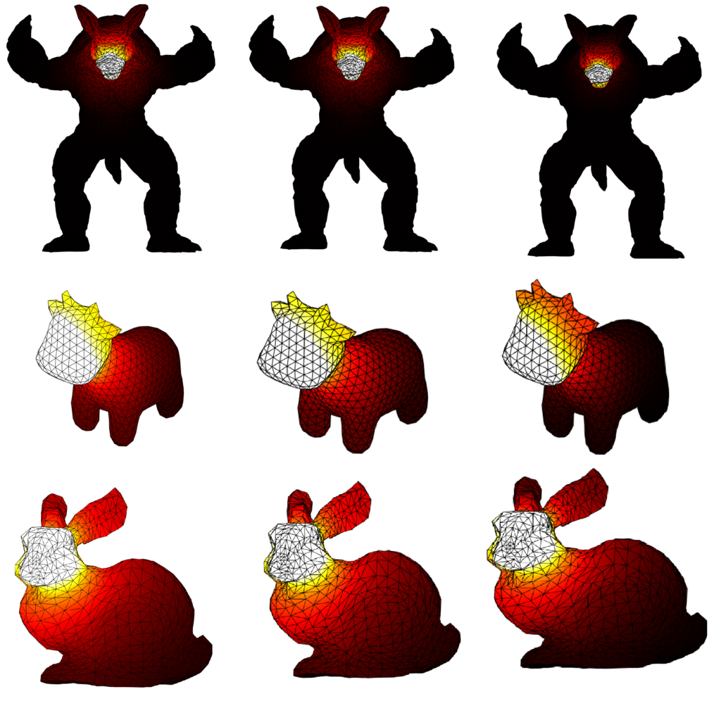
Here we try 2 simple algorithms that use the Cotan Laplacian and the Mass matrix. The first is solving a simple Poisson equation that finds a smooth density function over the mesh vertices given some fixed density values on a few of them. The other one is the “(Modified) Mean Curvature Flow” [11]. This flow is used for Mesh Smoothing. the Figures above show these algorithms’ output on the stanford bunny mesh.

Fig. 22. A simple cone with an extremely skinny triangulation to test the effects of Mollification.

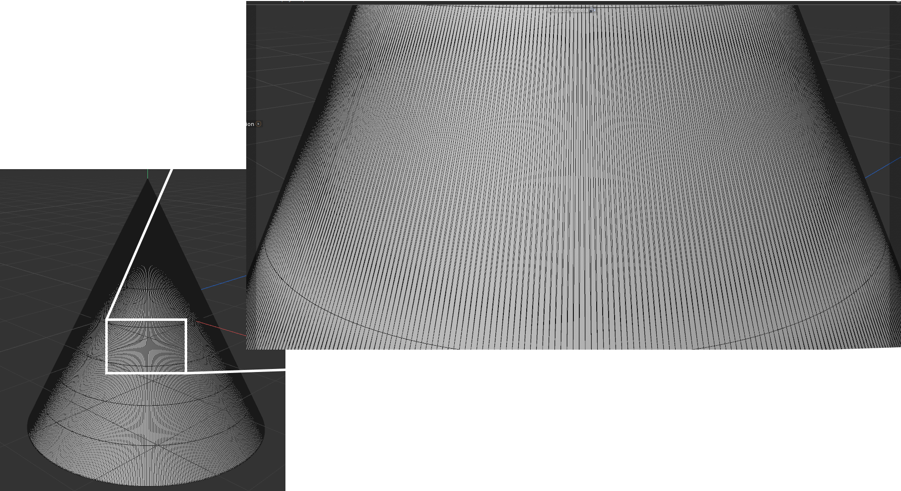
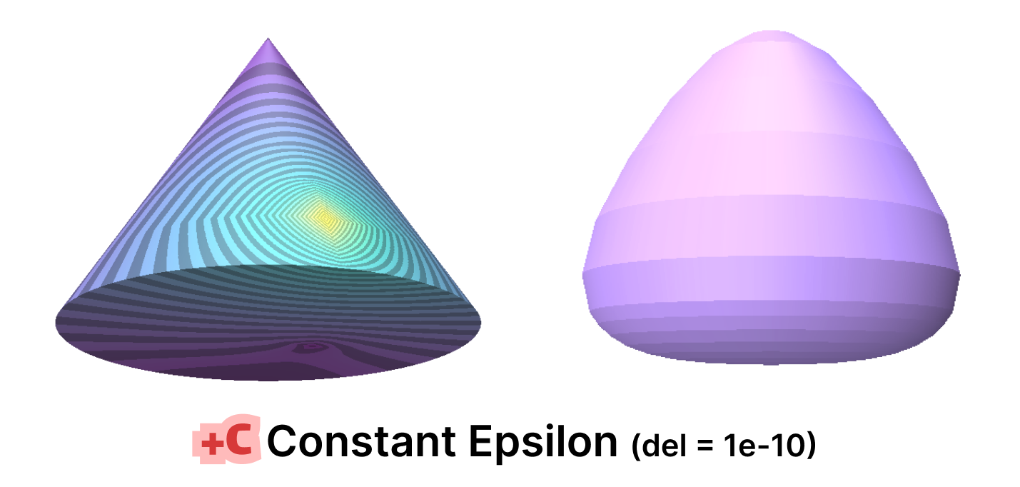
For purposes of quickly testing some applications with and without mollification, we generated a simple cone mesh segmented as, Rotation segments = 500, Height segments = 8, Cap segments = 8 (Shown above). Even though this is a mesh with simple shape and connectivity, it has a lot of skinny triangles. Without Mollification, running both algorithms on this mesh results in NaN values over the whole mesh. But with the slightest bit of Mollification (extremely small $\delta$ values like $10^{-10}$), the algorithms don’t crash and we can see reasonable results as shown below.

Fig. 23. The simple Constant Mollification with small $\delta$ is good enough for solving the NaNs issues that occur without Mollification.

It is worth noting that some combinations of the hacks earlier also produced similar results, some produced NaNs and others produced some results that are much less accurate. In general, it is not always clear which combination makes sense for the problem at hand.

5.5 Surface Parameterization

Fig. 24. A simple animation showing the 3D model of a Mountain being flattened to the UV plane. The **red** triangle is highlighted just to show how one triangle sits in the flattened mesh.

5.5.1 The Parameterization Problem

As defined by “Least squares conformal maps for automatic texture atlas generation” [12], the problem of parameterizing a surface $S \subset \mathbb{R}^3$ is defined as finding a correspondence between $S$ and a subset $S’ \subset \mathbb{R}^2$ by unfolding $S$. The animation above visualizes this “unfolding”. When the map $f: S \to S’$ locally preserves the angles, the map is said to be conformal.

5.5.2 Relevant Parameterization Algorithms

In order to preserve angles between $S$ and $f(S)$, it is possible to minimize the variation of tangent vectors from $S$. From [12], we can define an energy $E_{LSCM}$ based on vector variation and the variance prediction method of Least Squares, the energy of Least Squares Conformal Map as follows:

$E_{LSCM}(\textbf{u}, \textbf{v}) = \int_X \frac{1}{2} | \nabla \textbf{u}^\perp – \nabla \textbf{v} |^2 dA $

As discussed by “Spectral Conformal Parameterization” [13], the previous equation can be written in matrix form. Let $L_c$ denote the cotangent Laplacian matrix and $\textbf{u}, \textbf{v}$ be vectors so that $[\textbf{u}, \textbf{v}]^T A [\textbf{u}, \textbf{v}]$ is the area vector of the mesh, we have the LSCM energy as:

$ E_{LSCM}(\textbf{u}, \textbf{v}) = \frac{1}{2} [\textbf{u}, \textbf{v}]^T (L_c – 2A) [\textbf{u}, \textbf{v}]$

Fig. 25. To minimize this energy non-trivially, we can find the second smallest eignevalue (left) [SCP], or pin down 2 vertices (right) [LSCM].

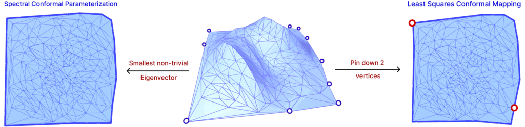
Hence, in order to minimize this energy, the gradient must be zero, that is, $Ax = 0$. However, since trivial solutions can be found in this optimization, two methods are used: pinning vertices and principal eigenvector of the energy matrix.

The idea of pinning two vertices is that one vertex will determine the global translation, while the other will determine the scaling and rotation, avoiding zeros in the Least Squares method. The other approach is to find the two smallest eigenvalues and eigenvectors of the energy matrix. Since a trivial solution is possible, the smallest eigenvalue is zero, then the second smallest eigenvalue and corresponding eigenvector will produce the minimization in question. The latter is a method called Spectral Conformal Parameterization (SCP). Both are shown in Figure. 25 above.

Fig. 26. Solving $\delta u = 0$ on the interior vertex positions results in a minimal surface subject to the boundary conditions.

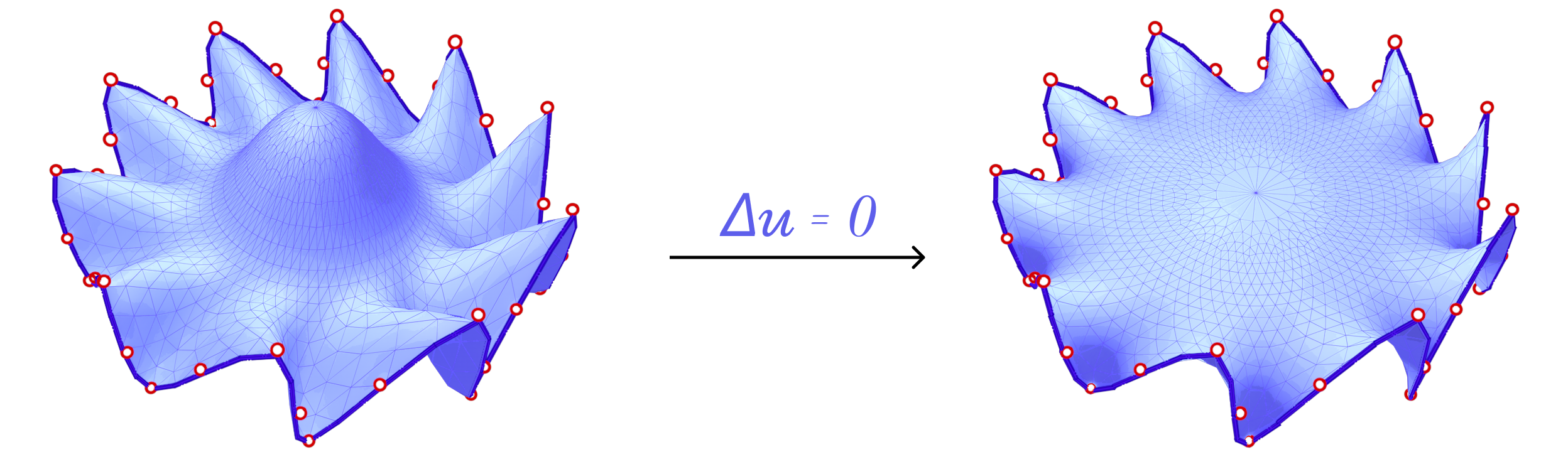
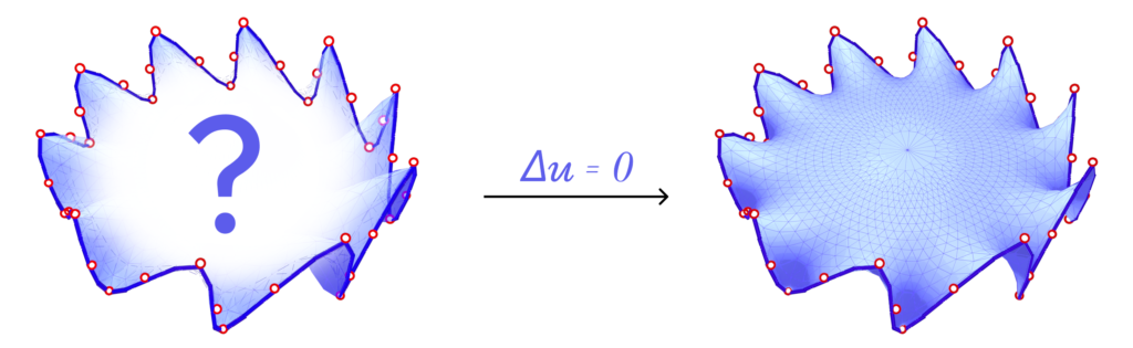
We also consider Harmonic Parameterization. This method is based on the idea of solving the Laplace equation on the surface $S$ with Dirichlet boundary conditions. That is, given a surface $S$ with all boundary vertices pinned, the Laplace equation $\delta z = 0$ is solved on the interior of $S$. Solving this equation results in a minimal surface as shown above.

Now, if we pin the boundary vertices to a closed curve in the plane, the resulting minimal surface would also be planar and the solution is the parameterization. In fact, since all boundary vertices are pinned, minimizing the harmonic energy is equivalent to minimizing the conformal energy mentioned above as the signed area term is constant for all possible parameterizations of $S$.

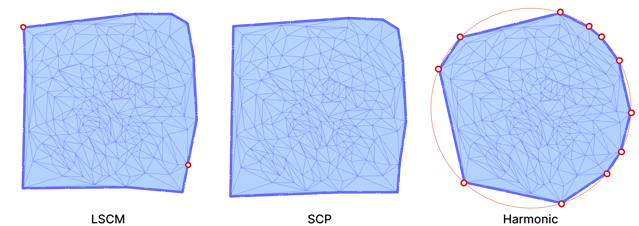
In all of our experiments, we pin the boundary vertices on a circle. The relative distances between consecutive boundary vertices are preserved in the parameterization. A Harmonic Parameterization of the same mount model is shown below side-by-side with LSCM and SCP.

Fig. 27. The output of applying the 3 parameterization algorithms on the 3D mount model side-by-side. The pinned-down vertices are colored in red. Both SCP and LSCM are similar to each other because they are both conformal maps.

All three algorithms use the cotangent Laplace matrix in their energy minimization process. Computing this matrix involves edge lengths and triangle areas. Therefore, they are good candidates for testing the effects of mollification when applied to bad meshes.

5.5.3 Evaluation Metrics & Methodology

In order to produce a technical comparison between the alternative hacks defined in Section 5.2 and Intrinsic Mollification, adequate measures are necessary. For this, we measure Quasi-conformal Distortion. This error metric (visualized below) is a measure of angle distortion for a given mapping and it is usually used to measure the quality of a Conformal Parameterization.

Fig. 28. The Quasi Conformal error on the parameterized faces resulting from the 3 different algorithms. The Harmonic mapping clearly has greater qc error values since it is not Conformal.

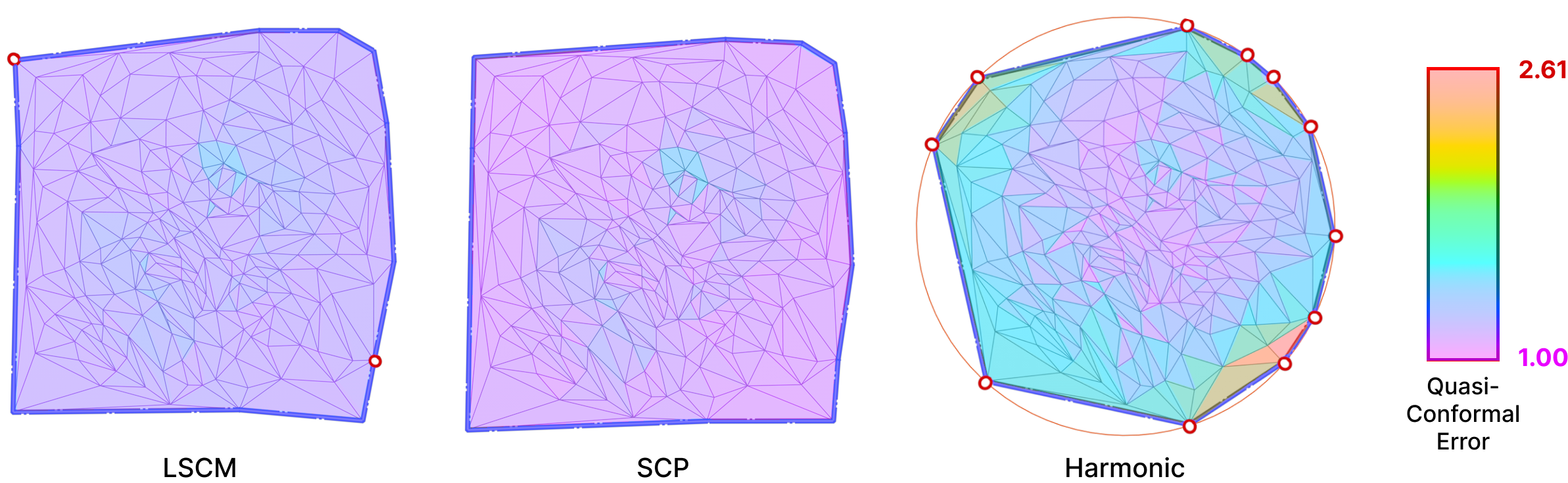
A best-case transformation is a triangle similarity. That is, shearing should be avoided to abstain the parameterization from distortion. For this, the Quasi-Conformal (QC) Error measures how close the original and final triangles are to a similarity. An error of $QC=1$ means that no shear happened. This can be used for comparing the distortion between the alternative strategies and the mollification.

For harmonic parameterization, we measure the relative area and length distortion instead of the QC error metric. This is because harmonic parameterization is not Conformal. Specifically, for one mesh, we compute this error as the norm of the vector of the (L1) normalized area (or length) differences before and after parameterization. In other words:

$e_{A} = | \frac{A_{param}}{|A_{param}|_1} – \frac{A_{o}}{|A_{o}|_1} |$,

$e_{L} = | \frac{L_{param}}{|L_{param}|_1} – \frac{L_{o}}{|L_{o}|_1} |$

Here, $A_{param}$ is a vector of face areas after parameterization (and potentially mollification), and $A_{o}$ is the same but of the original mesh. We normalize each before taking the difference to make sure the total area is equal. The norm of this difference vector is the metric we compute to see how areas are distorted. We also compute an isometry error metric which is computed in the same way but over lengths instead of areas.

Whenever the Laplacian has weights that are either negative or numerical zeros, it is common for a parameterization to produce flipped triangles. That is, a triangle which intersects other faces of the parameterized mesh. Then, a possible measure is to count the number of flipped triangles in the parameterized form. We tried this on a few meshes (but not across the dataset) to see how much mollification improves things and we found some promising results. It is worth trying this on a large-scale dataset to get more specific statistics in the future.

Fig. 29. A simple animation illustrating growing a patch from a sphere to apply the parameterization algorithms on it.

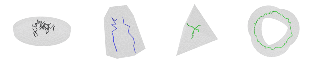
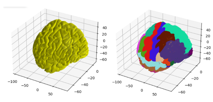
Parameterization requires the input mesh to have at least a boundary loop. It also zero genus (i.e. topologically equivalent to a sphere). Since most Thing10k meshes are solid objects with arbitrary genera, we implemented a simple algorithm to extract a genus-zero patch from the input mesh.

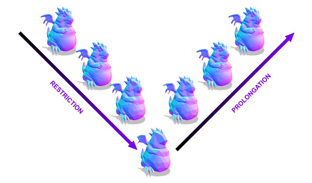
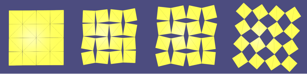
The algorithm is a simple Breadth-First-Search starting from a random face and visiting neighboring faces. This is equivalent to growing the patch by applying the $Star$ and $Closure$ operators ($Closure \circ Star$) repeatedly (as shown below). The algorithm stops when we reach a specified fraction of the total number of faces in the input mesh. Of course, this algorithm is not guaranteed to find a manifold genus-zero patch, but it is not costly to re-run it (with a bit smaller fraction and from a different face) until a valid patch is found. Most patches are found on the first or second try.

Fig. 30. Interleaving Star and Closure to grow the selection.

5.5.4 Benchmark Results

We ran the Conformal Mapping algorithms on the filtered Thingi10K dataset (~ 3400 meshes) and with with $\delta$ values $10^{-4}$ and $10^{-2}$. We report the median of Quasi-Conformal (QC) errors across all meshes as well as the number of times this metric function returned NaN or Inf values (indicating degenerate parameterizations like zero-area). The table below summarizes such results

Table 3. showing the Conformal Mapping benchmark results over 3400 meshes.

We immediately see an improvement in robustness. For all schemes and both mapping algorithms, about 62% of the cases where QC = NaN (or inf) were solved by mollification. This is independent of the chosen $\delta$ value. Of course, in some of these cases, it could be the case that our implementation of the QC error function is not robust enough (other than the mapping itself). But the effect of Mollification is clear nonetheless.

As for the QC error values, most schemes are generally close (and much better than no mollification), with the constant scheme being slightly better with smaller deltas and slightly worse with larger deltas. Overall, the more advanced schemes do not seem to make things better than the basic (constant) one for Conformal Parameterization. Here, it seems that smaller $\delta$ values like $10^{-4}$ seem to work better than larger values ($10^{-2}$).

Table 4. showing the Harmonic Mapping benchmark results over 2900 meshes.

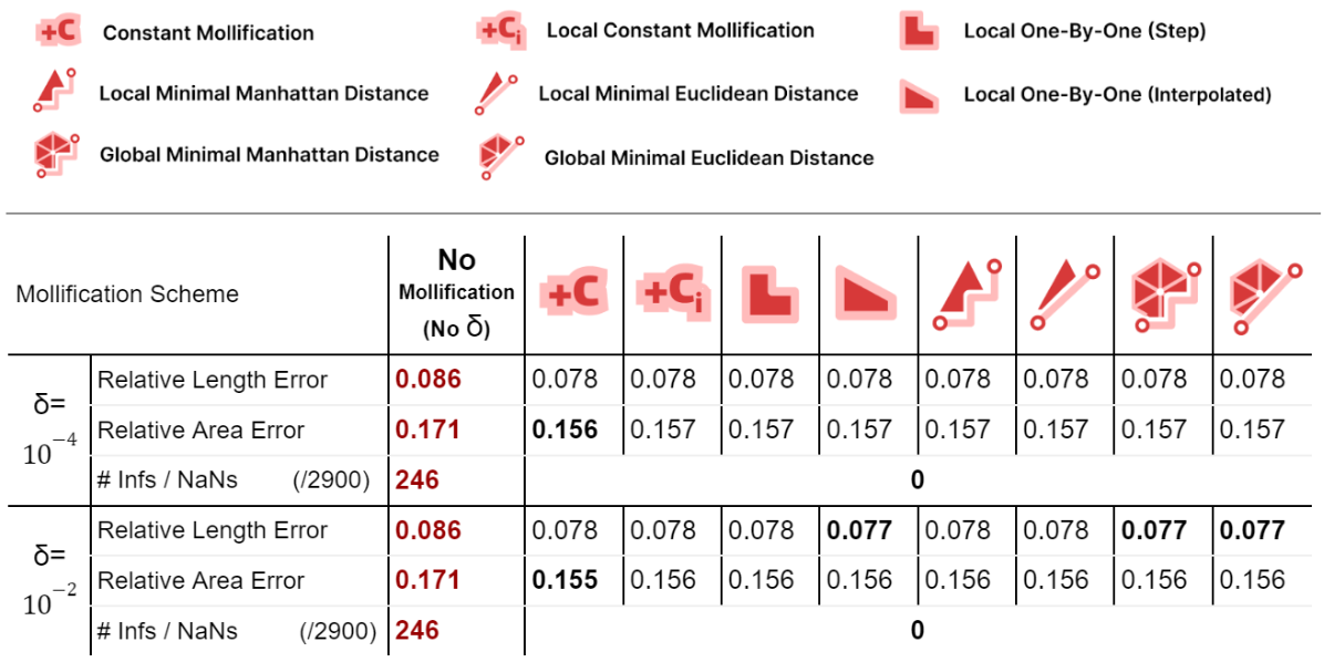
For harmonic mapping, all cases where the length error or area error where NaNs (or infinities) were solved by all schemes. As for the relative length and area errors, they seem to also improve significantly with mollification. And comparing the mollification schemes, they seem extremely close as well. Overall, ther isn’t a clear advantage of one scheme over the others.

We also ran benchmarks to compare these mollification schemes against the hacks. We first ran a small sample of the dataset on all combinations of the hacks mentioned in 5.2. There have been only two options that seemed to improve things significantly here. Namely, Replacing NaN/Infs with zeros or with ones. So, we ran the parameterization benchmarks again (on 3400 meshes) with these two options and without them, and compared that against 4 of the mollification schemes ($\delta = 10^{-4}$). The results are summarized in the table below.

Table 5. Comparing simple hacks against Intrinsic Mollification schemes, and the combination of both. Best values per row are in bold. Cases where a hack is clearly better than the 2 other options (for the same mollification scheme) are underlined with a **green** line.

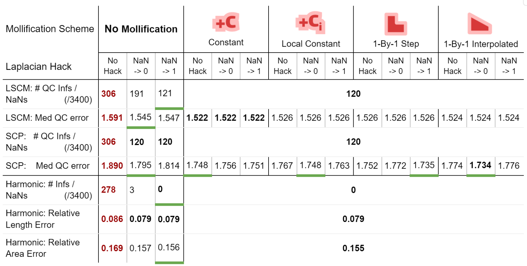
From the table, first, we see that the Nan-to-Zero hack isn’t reducing the cases of Qausi-Conformal error nearly as much as the Nan-to-One hack or the mollification schemes. Moreover, while both hacks reduce the Median of these errors, there is a clear advantage for all Mollifiction schemes. In fact, all of them reduce this metric by about $~ 50-60\%$ more on average than the hacks. From this, it is clear that Intrinsic Mollification has stronger effects on robustness than even the best-performing combinations of the tested hacks.

Another surprising result from the table is that combining Intrinsic Mollification with such simple hacks can be useful in some cases. For example, on local schemes in the table, the hacks sometimes even further improve the effect of mollification on the QC error. This shows that we can still use hacks after Mollification but it is not immediately clear when to use which hack because they can also harm the results.

Overall, for the parameterization benchmarks, there does not seem to be a clear advantage of the introduced Mollification schemes to the original constant one.

5.6 Geodesic Distance

5.6.1 The Geodesic Distance Problem

Fig. 31. A geodesic distance (**red**) between two points is the length of the shortest path between them on a curved surface (a Sphere patch in this example). This is different from the trivial Euclidean distance (**green**) and the graph distance (**purple**) that can be computed easily with algorithms like Dijkstra.

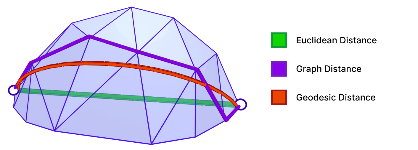
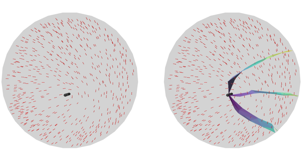
A Geodesic path represents the shortest (and straightest) path between two points on a surface. Geodesic distance is the length of such path. As shown above, the geodesic distance is different from the trivial Euclidean distance. Accurate computation of geodesic distance is important for many applications in Computer Graphics and Geometry Processing, including Surface Remeshing, Shape Matching, and Computational Architecture. For more details on geodesics and algorithms for computing them, we refer the reader to “A Survey of Algorithms for Geodesic Paths and Distances“[14].

5.6.2 The heat method for computing geodesic distance

Fig. 32. An animation showing the heat diffusion process on a sphere. For visualization purposes, the points with high heat values (**in bright yellow**) are moved far outwards from the center and the points with low heat values (**in red**) are moved inwards.

The idea of the heat method is based on the concept of heat diffusion. That is, given a surface $S$ with a heat distribution function $u_0$, the heat diffusion process is described by the heat equation:

$\frac{\partial u}{\partial t} = \Delta u$

where $\Delta$ is the Laplace-Beltrami operator. As time goes by, the heat distribution function $u$ will approach the steady state solution $u_\infty$ where $\frac{\partial u_\infty}{\partial t} = 0$.

Fig. 33. Showing the result of applying the heat method on the 3D mountain model. The heat source is the vertex at the top of the mountain (marked **in bright yellow**).

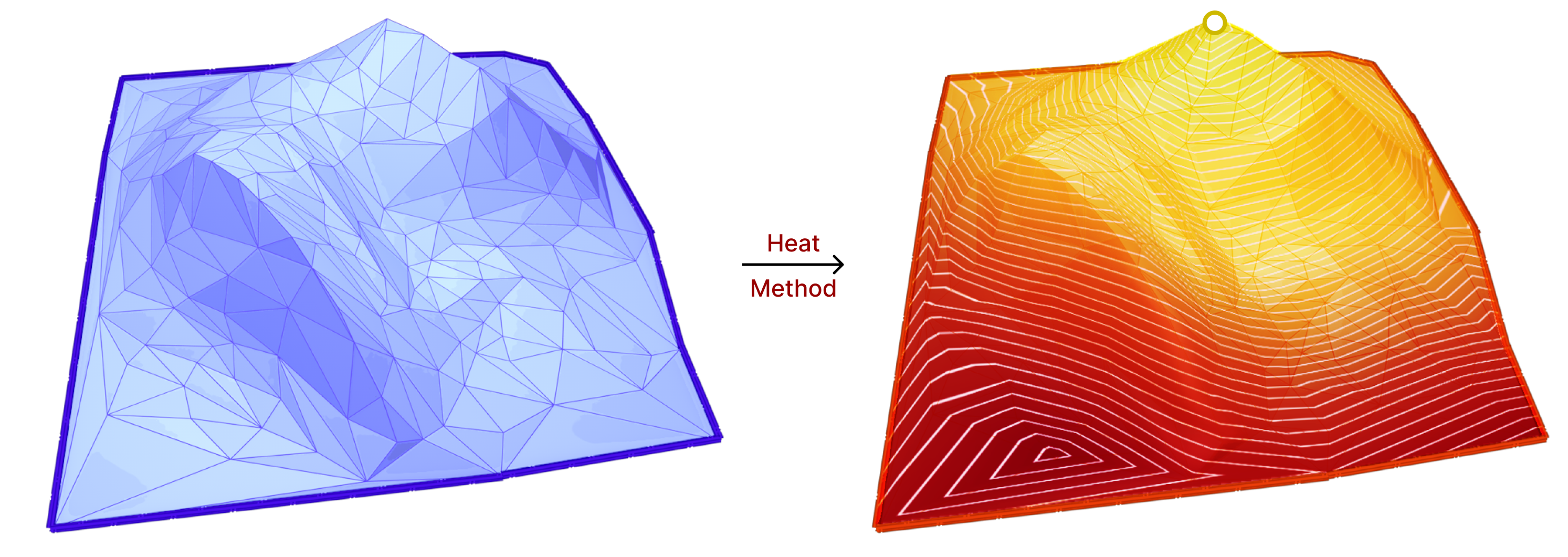
The heat method uses the heat diffusion process for a short period of time to compute the geodesic distance function. More specifically, the heat method consists of the following steps:

Initialize the heat distribution with heat source/s on surface vertices.
Let the heat diffuse for a short period of time. This involves solving the heat equation: $\frac{\partial u}{\partial t} = \Delta u$.
Compute the gradient of the heat distribution function $X = \nabla u$.
Normalize the gradient $X$.
Finally, solve a simple Poisson equation to obtain the geodesic distance function $\phi$.

$\Delta \phi = \nabla \cdot X$

From the above steps, we can see that the Laplace-Beltrami operator is used multiple times. Hence, this method is a good candidate to test the effects of our work on its accuracy. For more details on the heat method, we refer to “The Heat Method for Distance Computation“[15].

5.6.3 Evaluation Metrics

Fig. 34. The exact polyhedral distance algorithm finds geodesics by tracing over straight segments over triangle chains. The resulting geodesic curve is a straight line in the (isometrically) flattened view of the chain.

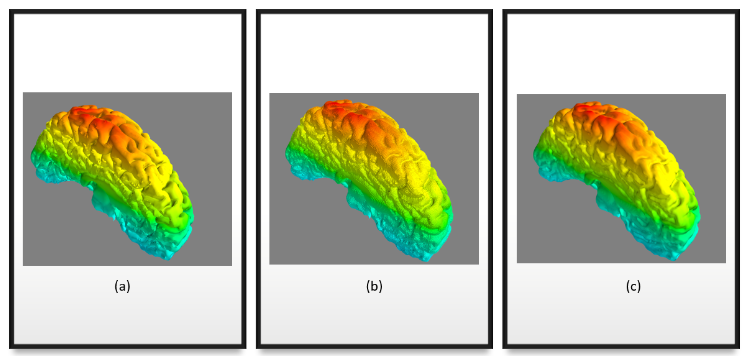
For evaluating the accuracy of the heat method, we use the exact polyhedral distance [16] function as a metric for comparison. The exact polyhedral distance metric provides the exact distance between two points on a polyhedral surface. Of course, the polyhedral mesh is an approximation of the original surface, so the exact polyhedral distance is not the same as the geodesic distance on the original surface. However, the exact polyhedral distance is a good enough approximation and it quickly gets closer to the geodesic distance of the original surface as the mesh resolution increases (quadratic convergence).

5.6.4 Benchmark Results

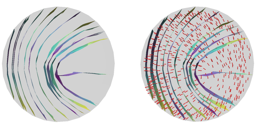
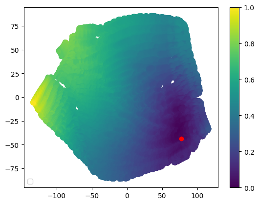
with the filtered Thingi10k meshes as a dataset, the exact polyhedral distance as a metric, the heat method was evaluated with mollification. We ran both of the algorithms with a random vertex as the source. We ran the benchmarks with different $\delta$ values $10^{-4}$ and $10^{-2}$, scaled by the average edge length of the mesh. The results are summarized below:

Table 6. The table summarizes the results of the heat method benchmark.

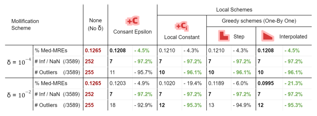
To measure accuracy, we computed the error as the Mean Relative Error (MRE) between the polyhedral distance and the heat method’s distance for each mesh. Since we are doing Single Source Geodesic Distance (SSGD), this is the mean of relative errors for all vertex distances from the source. We report the median of such MREs (Med-MREs) as a measure of how well each algorithm does on the whole filtered dataset (more than 3500 meshes).

There is an immediate improvement in accuracy using any Mollification algorithm in comparison to applying the heat method without any. In particular, for $\delta = 10^{-4}$, we can see about $~ 4.5\%$ of similar improvement for all schemes compared to no-mollification. This is true as well for smaller values like $10^{-5}$ and $10^{-6}$.

For large delta values ($\delta = 10^{-2}$), we can see that the local schemes produce significantly better results than the constant scheme (and no-mollification); Reaching an improvement of (~$21.3\%$) for the Median of MREs on the One-By-One Interpolated Scheme.

An important note is that we ran benchmarks multiple times with slightly different configurations. In some cases, the One-By-One Step scheme did better than the Local Constant One. But it was almost always the case that One-By-One Interpolated Scheme was a bit better than others for large $\delta$.

In addition to MRE, we count the number of times the heat method produces infinity or NaN values (which is an indication of failure) as #inf | NaN. We also count the number of times where $MRE > 100\%$. This is reported as #Outliers. It also includes in its count the times infinity or NaN values were produced.

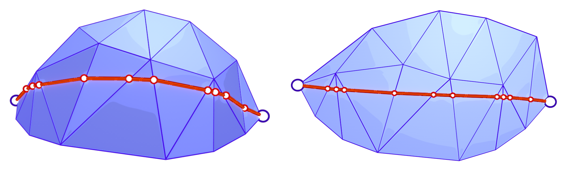
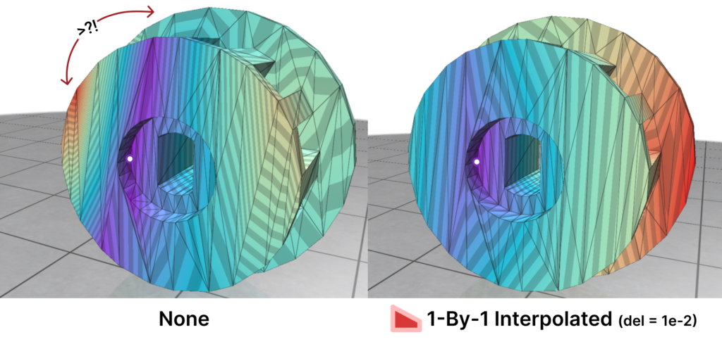
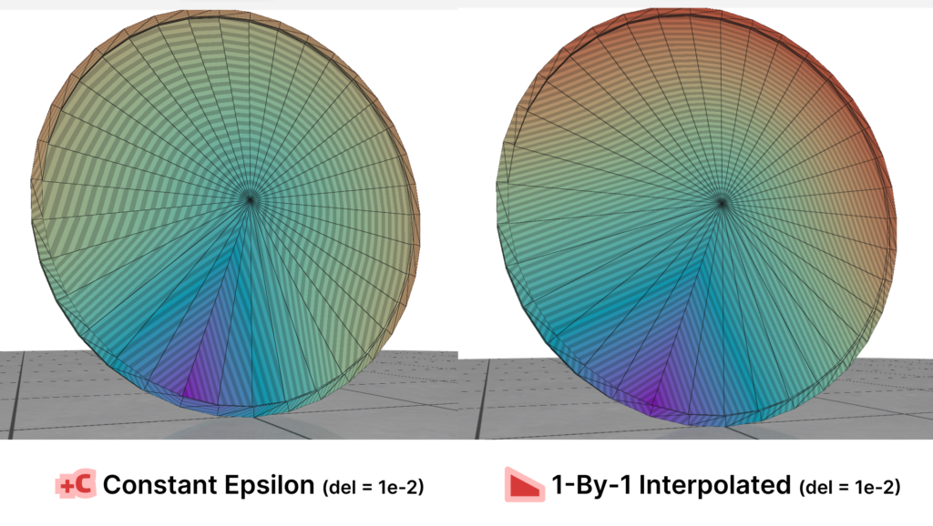
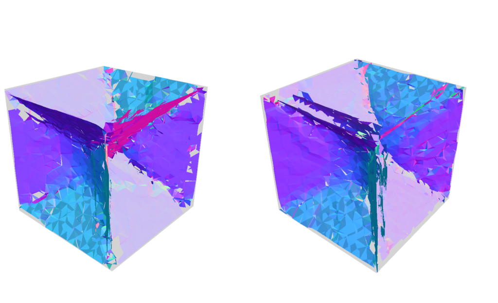
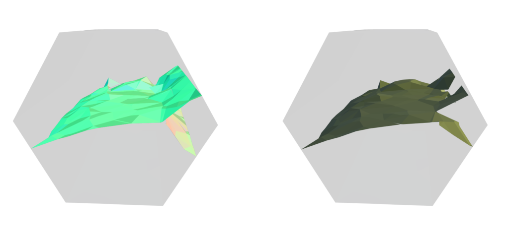
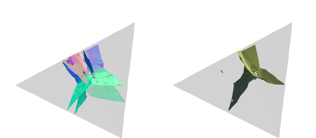
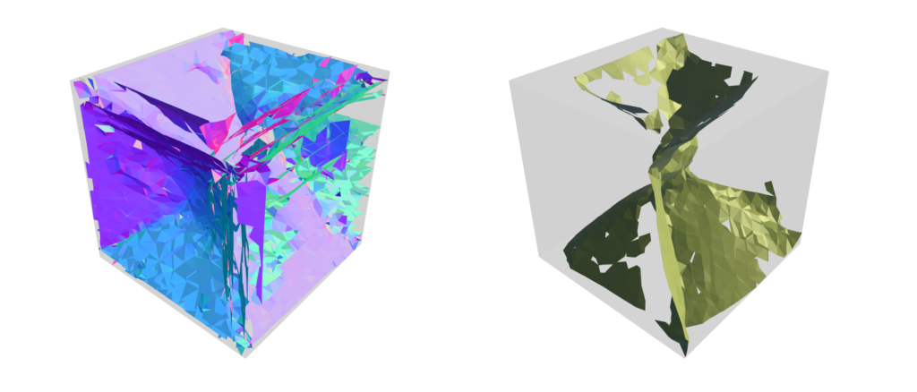
Here is where Intrinsic Mollification truly shines; running the heat method implementation on the dataset directly results in about $~ 252 / 3589$ failing cases (Infinities or NaNs). But, with the slightest mollification, 97% of these cases work fine. This is true for smaller values of $\delta$ that aren’t shown in the table too (like $10^{-6}$). As for outliers, we notice that the Local Mollification algorithms tend to produce fewer outliers on average than the Constant Mollification scheme, especially when $\delta$ is larger. The images below show some examples of the Outliers.

Fig. 35. Outliers.1: In some meshes, The results without mollification can be very wrong due to skinny triangles. Here distances are highly distorted some of the closest points having the largest distance as shown. With Mollification, these results look significantly better.

Fig. 36. Outliers.2: Here we can see that in some cases and even for reasonable meshes, the Constant scheme produces outliers. The resulting distance function looks discontinuous and the distances are distorted. But the Local schemes can produce much more reasonable results. This was also tried on smaller $\delta$ values and the results were similar.

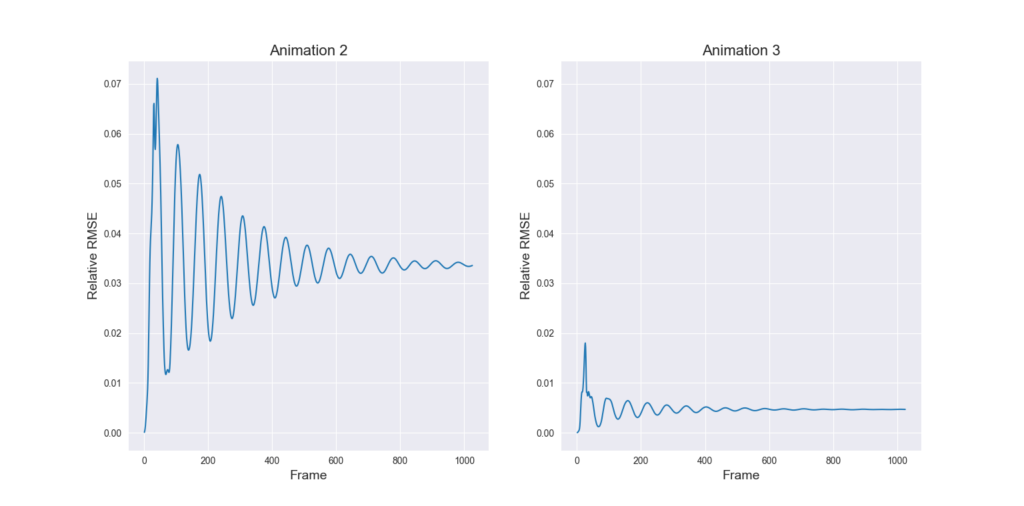
We ran this with and without the total length normalization step mentioned in 4.7. it had almost no effect on most of the mollification schemes. It is also interesting to see the behavior of each Mollification scheme with different $latex\delta$ values. Is there a best value for this parameter? The graph below shows this.

Fig. 37. The graph compares the effect of different $\delta$ values on the mollification algorithms performance in terms of the median of Mean Relative errors on geodesics.

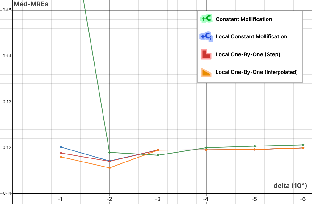
At least for the Heat method, one realization is that the local schemes allow higher $\delta$ values than the constant scheme before the results get unreasonable. This is most likely because the local schemes mollify only where it is needed and with much less length distortion overall. Another realization is that $10^-3$ and $10^-2$ seem like optimal $\delta$ values for the constant and local schemes respectively. We ran this benchmark a few different runs and with slightly different configurations but this fact seemed to hold for most runs.

As explained in the following section, we only ran this benchmark on the schemes shown in the table. It might be interesting to see how the others perform on the heat method. Also, we only ran these algorithms on meshes with atmost 20,000 faces to speed up the benchmark.

5.7 Notes on Implementation

we want to talk a bit about the benchmarks and the implementations of the heat method. we had trouble running/implementing it with Python and Libigl, so we switched to C++ and CGAL. We also had to rewrite the mollification algorithms in C++. Due to time constraints, we only managed to implement: the Constant, Local Constant, and Local 1-By-1 schemes. we think it would be interesting to try the other ones on the heat method and see their effects.

For the mollification schemes that use Linear or Quadratic programming, we used different solvers (SciPy and CvxOpt respectively). This makes the performance comparison between them questionable. Moreover, there might be other more time-efficient solvers. It would be interesting if that would increase the performance significantly.

6. Conclusions, Limitations, and Future Work

6.1 Conclusions

Table 7. Summarizing the comparison between the different mollification schemes.

Based on all benchmarks applied, it is clear that Intrinsic mollification can make algorithms using the Cotan-Laplace matrix much more robust, especially against extremely skinny triangles. Moreover, it seems that the simple “bad-value” replacement hacks are not as effective.

As for comparing the newly introduced Mollification schemes with the original one, They aim to reduce the amount of added length, and succeed remarkably at that, decreasing the distortion in geometry greatly. This is an important result; because some applications and algorithms might require harder guarantees on (intrinsic) triangle quality. Thus, a higher $\delta$ value can be used to achieve that without distorting triangles that are already in good shape.

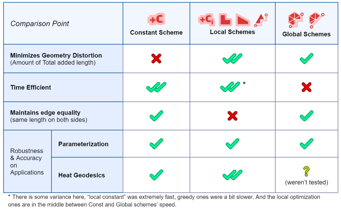
Some of the Introduced schemes are global and highly time-expensive. However, the local schemes are reasonably fast and reduce added length most effectively among all mollification schemes.

Running these on the parameterization algorithms, all these schemes do not make any improvements over the constant scheme. On the other hand, It is true that on some algorithms (like the heat method), the local schemes do improve things quite remarkably.

6.2 Limitations

Intrinsic Mollification is a good pre-processing step because it is very simple and fast. But this is also the reason it is very limited; In particular, there’s only so much improvement you can hope to get by just changing edge lengths. For instance, if you don’t have enough resolution in one part of the mesh (or you have too much resolution), mollification won’t help.

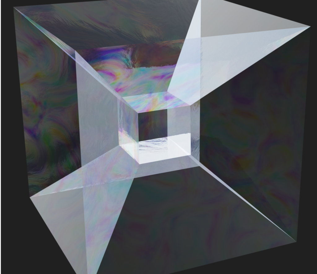
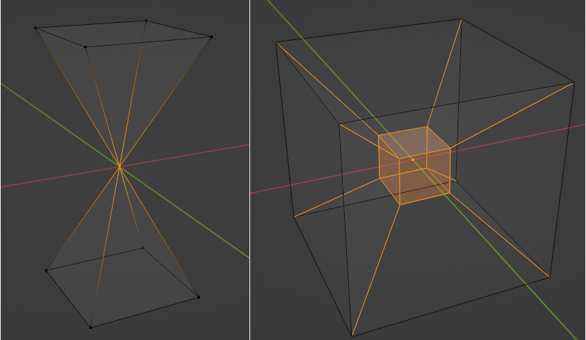
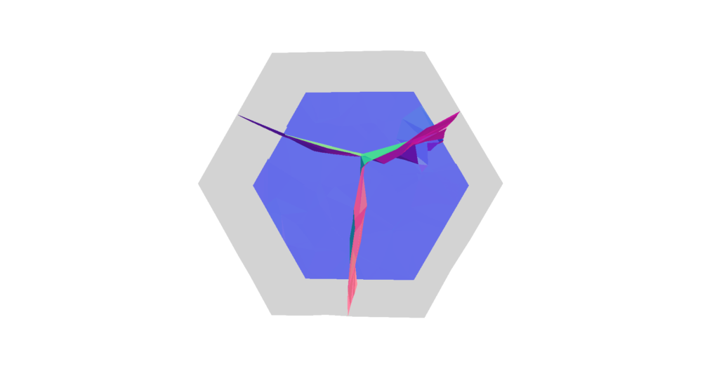
there is also a trade-off between (intrinsically) better triangles and distorting the geometry too much. A simple example is having a cone vertex with very high valence which would get very distorted as shown below.

Fig. 38. This shows a tall Cone ($height = 5 \pi * diameter$) with 200 faces around the top vertex (left). We can see the effect of Mollification ($\delta = 10^{-2}$) on the intrinsic lengths, making base segments x10 times larger and distorting the geometry greatly.

Lastly, In order to greatly reduce the amount of added length and only do that where it is needed, the local schemes sacrifice having the same edge length on both sides of the same edge. The Global schemes we worked on to solve this were either very slow (Linear/Quadratic programs over the whole mesh), or do not converge (sequential pooling schemes). So there is not one clear option that is fast, reliable, does not distort the geometry too much, and keeps edge lengths unbroken. However, that last property does not seem to practically affect the performance. So, some of the local schemes seem to be a favorable choice for a lot of applications.

6.3 Future Work

The work on this project was done in a very short period of time. So, we were not able to explore all the ideas we thought were promising. For example, If we find pooling operations that guarantee the Sequential Pooling schemes converge, then they can be much better alternatives than the global optimization schemes since those are very slow. Moreover, we would get a wide range of variants as we can use any of the local schemes as steps before each pooling iteration. We might even be able to compose such operations in interesting ways.

In this project, we only explored the effects of Mollification on the Laplacian. But it might be useful to apply Mollification before other types of computations where skinny and near-degenerate triangles harm robustness and accuracy and see if Mollification is effective in such cases.

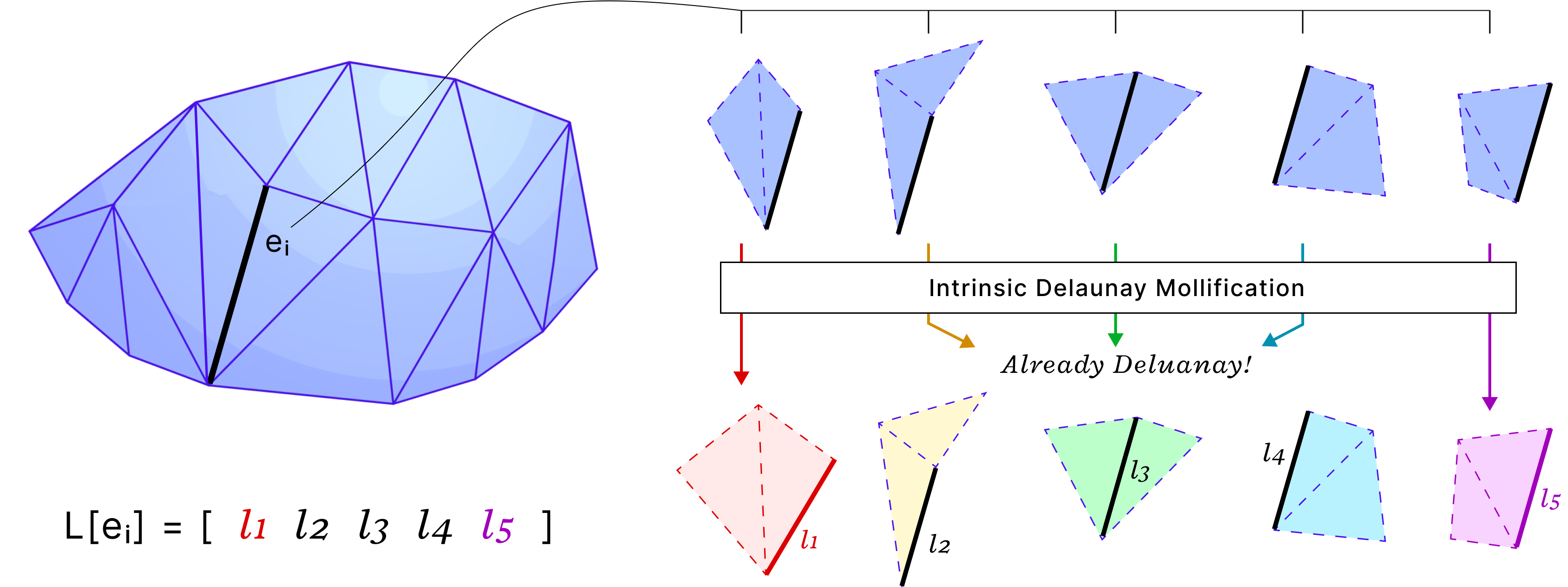
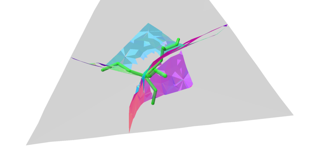
the idea of Intrinsic Mollification is fresh and very flexible. Local schemes even reduce restrictions on the usage of this concept. Hence, we can try to find other usages (and formulations) than fixing skinny triangles. One example is “Intrinsic Delaunay Mollification”. Where we would consider the neighborhood of each edge, (locally) Mollify the 5 involved edge lengths so that the Delaunay condition is satisfied with the least amount of added length. In that case, each edge would have different lengths, but each one would be used in the appropriate iteration of edges around it. The figure below shows a sketch of this idea.

Fig. 39. Intrinsic Delaunay Mollification? We can mollify edge lengths (locally) to get to satisfy the Delaunay condition. In this example, 3 edge neighborhoods already satisfy it with no mollification.

For the Local schemes, it might be worth trying to optimize their time performance by vectorized operations or parallelization. They are relatively fast, but there is some room for optimization there.

As mentioned in 4.7, normalizing to keep some properties unchanged may be a good idea to maintain certain aspects of the shape. Implementing the right normalization operation for the application might indeed be rewarding. One example to try is maintaining the same total area.

One of the most promising ideas is to try to apply this concept to Tetrahedral meshes. Tetrahedral meshes are often used in simulations, material analysis and deformations. These computations can behave poorly with bad-quality tetrahedrons. So, it is a great opportunity to apply the same concepts to this representation. Here, the problem is no longer just linear inequalities, but now we also have a nonlinear determinant condition (Cayley–Menger determinant). Nonetheless, it is a very interesting direction to put some effort into.

References

[1] Sharp Nicholas and Crane Keenan. 2020. A laplacian for nonmanifold triangle meshes. In Computer Graphics Forum, Vol. 39. Wiley Online Library, 69–80.

[2] Jonathan Richard Shewchuk. What Is a Good Linear Finite Element? Interpolation, Conditioning, Anisotropy, and Quality Measures, unpublished preprint, 2002.

[3] Khan, Dawar & Plopski, Alexander & Fujimoto, Yuichiro & Kanbara, Masayuki & Jabeen, Gul & Zhang, Yongjie & Zhang, Xiaopeng & Kato, Hirokazu. (2020). Surface Remeshing: A Systematic Literature Review of Methods and Research Directions. IEEE Transactions on Visualization and Computer Graphics. PP. 1-1. 10.1109/TVCG.2020.3016645.

[4] Fisher, M., Springborn, B., Schröder, P. et al. An algorithm for the construction of intrinsic Delaunay triangulations with applications to digital geometry processing. Computing 81, 199–213 (2007).

[5] Nicholas Sharp, Yousuf Soliman, and Keenan Crane. 2019. Navigating intrinsic triangulations. ACM Trans. Graph. 38, 4, Article 55 (August 2019).

[6] N Sharp, M Gillespie, K Crane. Geometry Processing with Intrinsic Triangulations. SIGGRAPH’21: ACM SIGGRAPH 2021 Courses.

[7] K Crane. 2018. Discrete differential geometry: An applied introduction. Notices of the AMS, Communication 1153.

[8] Zhou, Qingnan and Jacobson, Alec. “Thingi10K: A Dataset of 10,000 3D-Printing Models.” arXiv preprint arXiv:1605.04797 (2016).

[9] Georgia Shay, Justin Solomon, and Oded Stein. A dataset and benchmark for mesh parameterization, 2022., Vol. 1, No. 1, Article. Publication date: October 2023.

[10] Ligang Liu, Chunyang Ye, Ruiqi Ni, and Xiao-Ming Fu. Progressive parameterizations. ACM Trans. Graph., 37(4), jul
2018.

[11] Michael Kazhdan, Jake Solomon, & Mirela Ben-Chen. (2012). Can Mean-Curvature Flow Be Made Non-Singular?.

[12] Bruno Lévy, Sylvain Petitjean, Nicolas Ray, and Jérome Maillot. Least squares conformal maps for automatic texture
atlas generation. ACM Trans. Graph., page 362–371, jul 2002.

[13] Mullen, P., Tong, Y., Alliez, P., & Desbrun, M. (2008, July). Spectral conformal parameterization. In Computer Graphics Forum (Vol. 27, No. 5, pp. 1487-1494). Oxford, UK: Blackwell Publishing Ltd.

[14] Keenan Crane, Marco Livesu, Enrico Puppo, & Yipeng Qin. (2020). A Survey of Algorithms for Geodesic Paths and Distances. arXiv preprint arXiv:2007.10430

[15] Crane, K., Weischedel, C., & Wardetzky, M. (2017). The Heat Method for Distance Computation. Commun. ACM, 60(11), 90–99.

[16] Mitchell, J., Mount, D., & Papadimitriou, C. (1987). The Discrete Geodesic Problem. SIAM Journal on Computing, 16(4), 647-668.

Post author By Hossam Mohamed Saeed
Post date October 17, 2023
Tags cotan-Laplace, geodesic distance, geometry processing, intrinsic triangulations, Parameterization, preprocessing, SGI project

Research

Reconstruction of Implicit Non-Manifold Surfaces

Post author By Matheus da Silva Araujo
Post date October 17, 2023
No Comments on Reconstruction of Implicit Non-Manifold Surfaces

I. Introduction

The majority of surfaces in our daily lives are manifold surfaces. Roughly speaking, a manifold surface is one where, if you zoom in close enough at every point, the surface begins to resemble a plane. Most algorithms in computer graphics and digital geometry have historically been tailored for manifold surfaces and fail to preserve or even process non-manifold structures. Non-manifold geometries appear naturally in many settings however. For instance, a dress shirt pocket is sewn onto a sheet of underlying fabric, and these seams are fundamentally non-manifold. Non-manifold surfaces arise in nature in a variety of other settings too, from dislocations in cubic crystals on a molecular level, to the tesseract structures that appear in real world soap films (see Figure 1) [Ishida et al. 2020, Ishida et al. 2017].

Figure 1: Soap film covering the non-manifold minimal surface of a tesseract structure.

The study of soap films connects very closely to a rich vein of study concerning the geometry of minimal surfaces with boundary. The explicit representation of minimal surfaces has a rich history in geometry processing, dating back to the classic paper by Pinkall and Polthier 1993 . Since then, there has been continued study within computer graphics for robust algorithms for computing minimal surfaces, something which is broadly referred to as “Plateau’s Problem”.

Recent work in computer graphics [Wang and Chern 2021] introduced the idea of computing minimal surfaces by solving an “Eulerian” style optimization problem, which they discretize on a grid. In this SGI project, we explored an extension of this idea to the non-manifold setting.

II. Surface Representations

There are multiple ways to digitally represent surfaces, each one with different properties, advantages and disadvantages. Explicit surface representations, such as surface meshes, are easy to model and edit in an intuitive way by artists, but are not very convenient in other settings like constructive solid geometry (CSG). In contrast, implicit surfaces allow to perform morphological operations, and recent advances, such as neural implicits, are also exciting and promising [Xie et al. 2022].

One practical advantage of explicit surface representations like triangle meshes is that they are flexible and intuitive to work with. Triangle meshes are a very natural way to represent manifold surfaces, i.e. surfaces that satisfy the property that the neighborhood of every point is locally similar to the Euclidean plane (or half-plane, in the case of boundaries), and many applications, like 3D printing, require target geometries to be manifold. Triangle meshes can naturally capture non-manifold features as well by including vertices that connect otherwise disjoint triangle fans as in (Figure 2, left) or by edges that are shared by more than two faces (Figure 2, right).

Figure 2: Examples of non-manifold meshes. Non-manifold vertices and edges are highlighted in orange. Left: mesh containing a non-manifold vertex. Right: mesh containing non-manifold edges. Blender highlights faces composed solely by non-manifold edges.

However, in many real world settings, geometric data is not naturally acquired as or represented by a triangle mesh. In applications ranging from medical imaging to constructive solid geometry, the preferred geometric representation is as implicit surfaces.

In 2D, implicit surfaces can be described by a function $f: \mathbb{R}^{2} \rightarrow \mathbb{R}$ that is described by the points $(x, y) \in \mathbb{R}^{2}$ such that $f(x, y) = c$ for some real value $c$. By varying the values of $c$ a set of curves, called level sets, can be used to represent the surface. Figure 3 shows two representations of the same paraboloid, one using an explicit triangle mesh representation (left) and one using level sets of the implicit function (right).

Figure 3: Two distinct representations of the same surface. Left: explicit representation of a hyperboloid using a surface mesh. Right: implicit representation of a hyperboloid using level sets.

While non-manifold features are naturally represented in explicit surface representations, one limitation of implicit surfaces and level sets is that they do not naturally admit a way to represent geometries with non-manifold topology and self-intersections. In this project we focused on studying a way of representing implicit surfaces based on the mathematical machinery of integrable vector fields defined on a background domain.

III. Representing Implicit Surfaces as Integrable Vector Fields

In this project our goal was to explore implicit representations of non-manifold surfaces. To do this, we set out to represent implicit function implicitly, as an integrable vector field.

A vector field $V: \mathbb{R}^{m} \rightarrow \mathbb{R}^{n}$ is a function that corresponds a vector for each point in space. In our case, we are interested in cases where $m = n = 2$ or $m = n = 3$; see Figure 4 for an illustration of a vector field defined on a surface.
Vector field design and processing is a vast topic, with enough content to fill entire courses on the subject – we refer the interested reader to Goes et al. 2016 and Vaxman et al. 2016 for details.

Figure 4: Vector field defined on a surface. Source: Goes et al. 2016.

One way of thinking of implicit surfaces is as constant valued level sets of some scalar function defined over the entire domain. Our approach was to represent this scalar function as a function of a vector field which we received as an input to our algorithm.

To reconstruct a scalar field from the vector field, it is necessary to integrate the field, which led us into the discussion of integrability of vector fields. A vector field is integrable when it is the gradient of a scalar function. More precisely, the vector field $V$ is integrable if there is a scalar function $f$ such that $V = \nabla f$.

Since it can be arbitrarily hard to find the function $f$ such that $V = \nabla f$, or this function may even not exist at all, an equivalent but more convenient condition to check if a vector field is integrable is whether the vector field it is curl-free, that is, if $\nabla \times V = 0$ for all points in space (Knöppel et al. 2015, Polthier and Preuß 2003). If the vector field is not curl-free, then it is non-integrable, and there is no $f$ such that $V = \nabla f$. A possible approach to remove non-integrable features is to apply the Helmholtz-Hodge decomposition, which decomposes the field $V$ into the sum of three distinct vector fields:

$\begin{equation} V = F + G + H \end{equation}$

such that $F$ is curl-free, $G$ is divergence-free and $H$ is a harmonic component. The curl-free $F$ component is integrable. Figure 5 visualizes this decomposition.

Figure 5: Helmholtz-Hodge decomposition of a vector field defined over a surface. Source: Adapted from Goes et al. 2016.

The non-integrable regions of the vector field correspond to regions where the vector field vanishes or is undefined, also called singularities. For a standard vector field, singular points can be located by checking if the Jacobian is a singular matrix. For implicit non-manifold surfaces, removing the singularities using Helmholtz-Hodge decomposition is not particularly interesting, because the singularities are the cause of the non-manifold features that we want to preserve. At the same time, the singularities prevent the integration of the field, which we wanted to do to reconstruct the levels sets of the implicit function. This dichotomy suggests two different approaches to reconstructing the surface, as described in Section V.

IV. Representing Non-Manifold surfaces as Integrable Frame Fields

Frame Fields or poly-vector fields are generalizations of vector fields which store multiple distinct directions at each point. This terminology was introduced to the graphics literature by Panozzo et. al. 2014, and a technique for generating such integrable fields was presented by Diamanti et. al. 2015.

Animation 1 illustrates one curious phenomenon related to the topology of directional and frame fields. Assume each direction is uniquely labelled (e.g., each different direction is assigned a different color). If you start labelling an arbitrary direction and smoothly circulates around the singularity, trying to consistently label each direction with a unique color, this necessarily causes a mismatch between the initial label and the final label at the starting point. As can be seen in the last frame of the animation, a flow line that was initially assigned a green color was assigned a different color (red) in the last step, characterizing a mismatch between the initial and final label of that flow line. This happens for all the directions.

Animation 1: Failure to uniquely label each flow line direction around a singularity in a directional field. The initial flow line was labelled green. Source: Adapted from Knöppel et al. 2013.

V. Surface Reconstruction

The task can be specifically described as follows: given a frame field defined on a volumetric domain (i.e., a tetrahedral mesh), our goal is to reconstruct a non-manifold surface mesh that represents a non-manifold implicit surface. Two distinct approaches were explored: (i) stream surface tracing based on the alignment of the vector fields and (ii) Poisson surface reconstruction.

V.1. Stream Surface Tracing

The first approach consisted in using stream surfaces to represent the non-manifold surface. Stream surfaces are surfaces whose normal are aligned with one of the three vectors of the frame field. These types of surfaces are usually employed to visualize flows in computational fluid dynamics (Peikert and Sadlo 2009). Many ideas of the algorithm we explored are inspired by Stutz et al. 2022, which further extends the stream surface extraction with an optimization objective to generate multi-laminar structures for topology optimization tasks.

It is known that the gradient $\nabla f$ of a function $f$ is perpendicular to the level sets of the function (see Figure 6 for a visual demonstration). Therefore, if we had the gradient of the function, it would be possible to extract a surface by constructing a triangle mesh whose normal vectors of each face are given by the gradient of the function. The main idea of the stream surface tracing is that the input frame field can be used as an approximation of the gradient of the function that we are trying to reconstruct. In other words, the normal vector of the surface is aligned with one of the vectors of the frame field.

Figure 6: the gradient $\nabla f$ of a function $f$ is perpendicular to the level sets of $f$.

Animation 2 displays a step-by-step sequence for the first two tetrahedrons that are visited by the stream surface tracing algorithm, that proceeds as follows:

Choose an initial tetrahedron to start the tracing;
Compute the centroid of the first tetrahedron;
Choose one of the (three) vectors of the frame field as a representative of the normal vector of the surface;
Intersect a plane with the centroid of the tetrahedron such that the previous chosen vector is normal to this plane;
Choose a neighbor tetrahedron that shares a face with the edges that were intersected in the previous step;
For the new tetrahedron, compute the centroid and choose a vector of the frame field (similar to steps 2 and 3);
Project the midpoint of the edge of the previous plane into a line that passes through the centroid of the new tetrahedron.
Intersect a plane with the point computed in the previous step and the new tetrahedron.
Repeat steps 5 through 8 until all tetrahedrons are visited.

After repeating the procedure for all the tetrahedrons in the volumetric domain, a stream surface is extracted that tries to preserve non-manifold features.

Animation 2: Illustration of the main steps of the stream surface algorithm applied to the first two tetrahedra. This procedure is repeated for all tetrahedra in the volumetric domain.

V.1.1 – Results using Vector Fields

Animation 3 demonstrates the stream surface tracing algorithm for a frame field defined on a volumetric domain. In this case, it can be seen that the algorithm extracts a Möbius strip, which is a non-orientable manifold surface.

Animation 3: Stream surface tracing incrementally reconstructing a Möbius strip.

However, the Möbius strip is still a manifold surface and we want to reconstruct non-manifold surfaces. As an example of a surface with non-manifold structures, consider Figure 7. Figure 7, left, shows a frame field and the singularity graph associated with it, while Figure 7, right, presents the surface by the algorithm. The output of the algorithm is a surface mesh containing a non-manifold vertex in the neighborhood of the singular curve, indicating the non-integrability of the field.

Figure 7: Left: frame field and associated singular curve. Right: surface extracted using the surface tracing algorithm. Notice the formation of a T-junction in the neighborhood of the singular curve.

By applying the stream surface tracing algorithm starting from different tetrahedrons, it is possible to trace multiple level sets of the implicit non-manifold surface. Figure 8 displays the result of such procedure, where multiple strips were extracted corresponding to different level sets. Figure 8, right, shows the frame field together with the extracted surfaces: here, it is possible to notice that each vector is approximately normal to the surfaces. This was expected, since the assumption of the algorithm was that the frame field can be used as an approximation of the gradient of the function we want to reconstruct.

Figure 8: Left: reconstructed surfaces for different level sets of the function. Right: surfaces and the corresponding vector field. Notice how the vectors are roughly orthogonal to the level sets, as expected.

V.1.2. Volumetric Frame Fields: Working with Frame Fields in 3D volumes

Implicit functions, as described above, are real-valued functions with infinitely many values. To represent them on a computer, some sort of spatial discretization is necessary. Two common choices are to discretize the space using regular grids or unstructured meshes where each element is a triangle or a tetrahedron. This discretization corresponds to an Eulerian approach: for a fixed discretized domain, the values of the vector fields associated with the implicit functions are observed in fixed locations in space. In this project, tetrahedral meshes are used to discretize the space and fill the volume where the functions are defined.

A tetrahedral mesh is similar to a triangle mesh, but augmented with additional data for each tetrahedron. Formally, a tetrahedral mesh $\mathcal{M}$ is defined by a set ${\mathcal{V}, \mathcal{E}, \mathcal{F}, \mathcal{T}}$ of vertices, edges, faces and tetrahedrons, respectively. Each tetrahedron is composed of 4 vertices, 6 edges and 4 faces. The edges and faces of one tetrahedron may be shared with adjacent tetrahedrons, which allow to traverse the mesh. More importantly, this allows to define the vector field using the tetrahedral mesh as a background domain to discretize the function over this volumetric space.

As input, we start with a boundary mesh enclosing a volume (Figure 9, top left). Bear in mind that this boundary mesh does not fill the space, but only specifies the boundary of a region of interest. We can fill the volume using a tetrahedral mesh (Figure 9, top right). This tetrahedralization can be done using Fast Tetrahedral Meshing in the Wild, for instance. It is important to notice that, in contrast to a surface polygon mesh, a tetrahedral mesh is a volume mesh in the sense that it fills the volume enclosed by it. If we slice the tetrahedral mesh with a plane (Figure 9, bottom left and bottom right), we can see that the interior of the tetrahedral mesh is not empty (as would be the case for a surface mesh) and that the interior volume is fully filled. In Figure 9, the interior faces of the tetrahedrons were colored in purple while the boundary faces were colored in cyan.

Figure 9: Tetrahedralization of a boundary domain. Starting with a boundary domain bounded by a surface mesh (top left), the domain is discretized using tetrahedrons (top right). Unlike a surface mesh, a volumetric mesh fills the interior space of the volume it discretizes (bottom row).

Three distinct vector fields $U, V, W$ constitute a volumetric frame field if they form an orthonormal basis at each point in space. As mentioned, we work with frame fields defined on a volumetric domain as a representation of the implicit non-manifold surface. Each tetrahedron will be associated with three orthogonal vectors, as shown in Figure 10.

Figure 10: Sample of data used to represent a non-manifold implicit surface. The domain was discretized using tetrahedral meshes (purple). Each tetrahedron is associated with three orthogonal vectors, that constitute a volumetric frame field.

The previous idea of labelling directions around a point can be useful to detect singularities in our frame fields. The same idea can be extended to volumetric frame fields, where singularities create singular curves on the volumetric domain. These curves are denominated as singularity graphs. Figure 11 shows the singularity graphs for some frame fields. See Nieser et al. 2011 for details. Identifying the singular curves on the frame fields is equivalent to identifying its non-integrable regions.

Figure 11: Singularity graphs of the volumetric frame fields.

V.1.3. Results using Volumetric Frame Fields

Another example is provided in Figure 12, where the volumetric frame field is defined on a hexagonal boundary mesh. The output presents a non-manifold junction through a non-manifold vertex.

Figure 12: reconstructed surface for a hexagonal boundary mesh.

As a harder test case, it can be seen in Figure 13 that the resulting surface extracted by the algorithm is not a perfectly closed mesh. While the surface tries to follow the singularity graph (in green), it fails to self-intersect in some regions, creating undesirable gaps.

Figure 13: reconstructed surface for a tetrahedral boundary mesh and the singularity graph (in green) associated with the volumetric frame field. The surface has an overall structure that resembles the junction present in the singularity graph, but in this case the algorithm wasn’t able to extract a mesh without holes.

Finally, we tested the algorithm to reconstruct the non-manifold minimal tesseract, presented in Figure 1. Two points of view of the output are presented in Figure 14. While the traced mesh has a structure similar to the desired surface, the result could still be further improved. The mesh presents cracks in the surface and some almost disconnected regions. We applied hole filling algorithms, such as those provided by MeshLab, as an attempt to fix the issue, but they weren’t capable of closing the holes for any combination of parameters tested.

Figure 14: reconstructed surface for the non-manifold minimal surface tesseract. The reconstruction preserves the overall structure of the desired surface. However, the algorithm fails to create a surface without holes and produces some regions that are mostly disconnected from the surface.

V.2. Poisson Surface Reconstruction

The second approach consisted in investigating the classic Poisson Surface Reconstruction algorithm by Kazhdan et al. 2006 for our task. Specifically, our goal was to evaluate whether the non-manifold features were preserved using this approach and, if not, where exactly it fails.

Given a differentiable implicit function $f$, we can compute its gradient vector field $G = \nabla f$. This can be done either analytically, if there is a closed-formula for $f$, or computationally, using finite-element methods or discrete exterior calculus. Conversely, given a gradient vector field $G$, we can integrate $G$ to compute the implicit function $f$ that generates the starting vector field.

Note that since it was assumed that $G$ is a gradient vector field, and not an arbitrary vector field, this means that $G$ is integrable. If this is the case, we know that a function $f$ whose gradient vector field is $G$ exists; we just need to find it. However, in practice, the input of the algorithm may be a vector field $V$ which is not exactly integrable due to noise or sampling artifacts. How can $f$ be computed in all these cases?

One core idea of the Poisson Surface Reconstruction algorithm consists in reconstructing $f$ using a least-squares optimization formulation:

$\begin{equation} \tilde{f} = \arg \min_{f} \left |V – \nabla f \right |^{2} \end{equation}$

For a perfectly integrable vector field (i.e., a gradient vector field), it would theoretically be possible to compute $\tilde{f} = f$ such that $\nabla \tilde{f} = V$ and reconstruct $f$ exactly. The advantage of this formulation is that even in cases where the vector field $V$ is not exactly integrable, it will reconstruct the best approximation of $f$ by minimizing the least-squares error.

In the case of our frame fields representing non-manifold surfaces, the existence of singularities in the field means that it will necessarily be non-integrable. It is expected that the equality $\nabla \tilde{f} = V$ fails precisely in the regions containing singular points, but we wanted to evaluate the performance of a classic algorithm on our data.

V.2.1 – Results using Volumetric Frame Fields

Figure 15 and Figure 16 present comparisons between the surface extracted by Stream Surface Tracing and Poisson Surface Reconstruction algorithm for two different inputs. While for the hexagonal boundary mesh (Figure 15) both algorithms have a similar output, for the tetrahedral boundary mesh (Figure 16) Poisson Surface Reconstruction generates a surface closer to the desired non-manifold junction.

Figure 15: Comparison between the Stream Surface Tracing algorithm (left) and the Poisson Surface Reconstruction (right) for the volumetric frame field with hexagonal boundary mesh.

Figure 16: Comparison between the Stream Surface Tracing algorithm (left) and the Poisson Surface Reconstruction (right) for the volumetric frame field with tetrahedral boundary mesh. In this case, Poisson Surface Reconstruction extracts a surface that is closer to the desired junction in comparison to the Stream Surface Tracing.

Remarkably, the Poisson Surface Reconstruction fails badly for the non-manifold tesseract, as shown in Figure 17. While the Stream Surface Tracing doesn’t extract a perfect surface reconstruction (Figure 17, left), it is much closer to the tesseract than the surface reconstructed by the Poisson Surface Reconstruction (Figure 17, right).

Figure 17: Comparison between the Stream Surface Tracing algorithm (left) and the Poisson Surface Reconstruction (right) for the volumetric frame field defined for the tesseract structure. In this case, Poisson Surface Reconstruction drastically fails to preserve the non-manifold structure of the target surface.

VI. Conclusions and Future Work

In this project we explored multiple surface reconstruction algorithms that could possibly preserve non-manifold structures from frame fields defined on tetrahedral domains. While the algorithms could extract surfaces that present the overall structure desired, for many inputs the mesh displayed artifacts such as cracks or components that aren’t completely connected, such as non-manifold vertices where a non-manifold edge was expected. As future work, we consider using the singularity graph to guide the tracing as an attempt to close the holes in the mesh. Another possible direction would be to explore the usage of the singularity graph in the optimization process used in the Poisson Surface Reconstruction algorithm.

I would like to thank Josh Vekhter, Nicole Feng and Marco Ravelo for the mentoring and patience to guide me through the rich and beautiful theory of frame fields. Furthermore, I would like to thank Justin Solomon for the hard work on organizing SGI and baking beautiful singular pies.

VII. References

Ishida, Sadashige, et al. “A model for soap film dynamics with evolving thickness.” ACM Transactions on Graphics (TOG) 39.4 (2020): 31-1.

Ishida, Sadashige, et al. “A hyperbolic geometric flow for evolving films and foams.” ACM Transactions on Graphics (TOG) 36.6 (2017): 1-11.

Pinkall, Ulrich, and Konrad Polthier. “Computing discrete minimal surfaces and their conjugates.” Experimental mathematics 2.1 (1993): 15-36.

Wang, Stephanie, and Albert Chern. “Computing minimal surfaces with differential forms.” ACM Transactions on Graphics (TOG) 40.4 (2021): 1-14.

Xie, Yiheng, et al. “Neural fields in visual computing and beyond.” Computer Graphics Forum. Vol. 41. No. 2. 2022.

De Goes, Fernando, Mathieu Desbrun, and Yiying Tong. “Vector field processing on triangle meshes.” ACM SIGGRAPH 2016 Courses. 2016. 1-49.

Vaxman, Amir, et al. “Directional field synthesis, design, and processing.” Computer graphics forum. Vol. 35. No. 2. 2016.

Knöppel, Felix, et al. “Stripe patterns on surfaces.” ACM Transactions on Graphics (TOG) 34.4 (2015): 1-11.

Polthier, Konrad, and Eike Preuß. “Identifying vector field singularities using a discrete Hodge decomposition.” Visualization and mathematics III. Springer Berlin Heidelberg, 2003.

Panozzo, Daniele, et al. “Frame fields: Anisotropic and non-orthogonal cross fields additional material.” Proceedings of the ACM TRANSACTIONS ON GRAPHICS (PROCEEDINGS OF ACM SIGGRAPH (2014).

Diamanti, Olga, et al. “Integrable polyvector fields.” ACM Transactions on Graphics (TOG) 34.4 (2015): 1-12.

Knöppel, Felix, et al. “Globally optimal direction fields.” ACM Transactions on Graphics (ToG) 32.4 (2013): 1-10.

Peikert, Ronald, and Filip Sadlo. “Topologically relevant stream surfaces for flow visualization.” Proceedings of the 25th Spring Conference on Computer Graphics. 2009.

Stutz, Florian Cyril, et al. “Synthesis of frame field-aligned multi-laminar structures.” ACM Transactions on Graphics (TOG) 41.5 (2022): 1-20.

Hu, Yixin, et al. “Fast tetrahedral meshing in the wild.” ACM Transactions on Graphics (TOG) 39.4 (2020): 117-1.

Nieser, Matthias, Ulrich Reitebuch, and Konrad Polthier. “Cubecover–parameterization of 3d volumes.” Computer graphics forum. Vol. 30. No. 5. Oxford, UK: Blackwell Publishing Ltd, 2011.

Kazhdan, Michael, Matthew Bolitho, and Hugues Hoppe. “Poisson surface reconstruction.” Proceedings of the fourth Eurographics symposium on Geometry processing. Vol. 7. 2006.

Post author By Matheus da Silva Araujo
Post date October 17, 2023
Tags 3D Reconstruction, Eulerian, frame fields, geometry processing, SGI project, Surface Reconstruction, tetrahedral mesh

Research

Multigrid Solver for Curved Surfaces

Post author By Matheus da Silva Araujo
Post date October 12, 2023
No Comments on Multigrid Solver for Curved Surfaces

Video 1: Numerical solution of the heat equation on curved meshes using a geometric multigrid solver.

By SGI Fellows: Anna Cole, Francisco Unai Caja López, Matheus da Silva Araujo, Hossam Mohamed Saeed

Mentor: Paul Kry

Volunteers: Leticia Mattos Da Silva and Erik Amézquita

I. Introduction

This technical report describes a follow-up to our previous post. One of the original goals of the project was to apply successive self-parameterization to solve differential equations on curved surfaces leveraging a multigrid solver based on Liu et al. 2021. This post reports the results obtained throughout the summer to achieve this objective and wraps-up the project. Video 1 shows an animation of heat diffusion, obtained by solving the heat equation on surface meshes using the geometric multigrid solver.

II. Partial Differential Equations

Partial differential equations (PDEs) are equations that relate multiple independent variables and their partial derivatives. In graphics and animation applications, PDEs usually involve time derivatives and spatial derivatives, e.g., the motion of an object in 3D space through time described by a function $f(x, y, z, t)$. Frequently, a set of relationships between partial derivatives of a function is given and the goal is to find functions $f$ satisfying these relationships.

To more easily study and analyze these equations, it is possible to classify them according to the physical phenomena they describe, which are briefly summarized below. Solomon 2015 and Heath 2018 provide extensive details on partial differential equations for those interested in more in-depth discussions on the topic.

Elliptic PDEs are PDEs that describe systems that have already reached an equilibrium (or steady) state. One example of elliptic PDE is the Laplace equation, given by $\bigtriangleup \mathbf{u} = \mathbf{0}$. Intuitively, starting with values known only at the boundary of the domain (i.e., the boundary conditions), this equation finds a function $\mathbf{u}$ such that the values in the interior of the domain smoothly interpolate the boundary values. Figure 1 illustrates this description.

Figure 1: Given boundary conditions, the Laplace Equation is satisfied by a function that smoothly interpolates it to the interior.

Parabolic PDEs are equations that describe systems that are evolving towards an equilibrium state, usually related to dissipative physical behaviour. The canonical example of a parabolic PDE is the heat equation, defined as $\frac{\mathrm{d}}{\mathrm{dt}} \mathbf{u} = \bigtriangleup \mathbf{u}$. The function $\mathbf{u}$ describes how heat flows with time over the domain, given an initial heat distribution that describes the boundary conditions. This behaviour can be visualized in Animation 1.

Animation 1: Given an initial heat distribution, the heat equation describes how heat flows over the surface as time progresses, until a steady state is reached.

Finally, hyperbolic PDEs describe conservative systems that are not evolving towards an equilibrium state. The wave equation, described by $\frac{\mathrm{d}^2}{\mathrm{dt^{2}}} \mathbf{u} = \bigtriangleup \mathbf{u}$, is the typical example of a hyperbolic PDE. In this case, the function $\mathbf{u}$ characterizes the motion of waves across elastic materials or the motion of waves across the surface of water. Animation 2 provides a visual illustration of this phenomenon. One striking difference between the wave equation and the heat equation is that for the former it is not enough to specify initial conditions for $\mathbf{u}$ at time $t = 0$; it is also necessary to define initial conditions for the derivatives $\mathbf{\frac{\mathrm{d}}{\mathbf{dt}} \mathbf{u}}$ at time $t = 0$.

Animation 2: Given initial boundary conditions for both the function and its first derivative, the wave equation describes the propagation of a wave through time.

In this project, we restricted the implementation to solving the heat diffusion equations on curved triangle meshes (see Crane et al. 2013). This leads to the following time discretization using a backward Euler step:

$\begin{equation} \frac{\mathrm{d}}{\mathrm{dt}} \mathbf{u} = \bigtriangleup \mathbf{u} \rightarrow (\mathbf{I} – t\mathbf{L}) \mathbf{u}_{t} = \mathbf{u}_{0} \end{equation}$

where $\mathbf{u}_{0}$ is the initial heat distribution and $\mathbf{L}$ is the Laplacian.

To spatially discretize the equation, we used the cotan-Laplacian $\mathbf{L}$ discretized at a vertex $i$:

$\begin{equation} (\mathbf{L}u){i} = \frac{1}{2 A_{i}} \sum_{j \in \mathcal{N}_{i}} \left(\cot \alpha_{ij} + \cot \beta_{ij} \right) \left(u_{j} – u_{i} \right) \end{equation}$

where $A_{i}$ is one-third of the sum of the areas of all the triangles incident to vertex $i$, $\mathcal{N}_{i}$ denotes the set of adjacent vertices, and $\alpha_{ij}, \beta_{ij}$ are the angles that oppose the edge $e_{ij}$ connecting vertex $i$ to its neighbor $j$. The result is a linear system $\mathbf{A}\mathbf{x} = \mathbf{b}$, where $\mathbf{A} = \mathbf{I} – t\mathbf{L}$ and $\mathbf{b} = \mathbf{u}_{0}$. This linear system can be solved numerically.

III. Multigrid Method

There is a large variety of methods to numerically solve PDEs. After choosing time and spatial discretization, the PDE may be solved as a linear system. To that end, it is possible to apply a direct solver (e.g., LU decomposition or Cholesky factorization) to find the solution. These methods are exact in the sense that they provide an exact solution in a finite number of steps. One disadvantage of direct solvers approach is that it may be too expensive to frequently recompute the matrix decomposition in cases where the system of equations requires updates. Iterative methods (e.g., Gauss-Seidel and Jacobi) provide an efficient alternative, but at the cost of providing only approximate solutions and having poor rates of convergence. Multigrid methods attempt to improve the convergence of iterative solvers by creating a hierarchy of meshes and solving the linear system in a hierarchical manner.

Iterative methods usually rapidly remove high-frequency errors, but slowly reduce low-frequency errors. This significantly affects the rate of convergence. The key observation of multigrid solvers is that low-frequency errors on the domain where the solution is defined (i.e., a grid or mesh) correspond to high-frequency errors on a \emph{coarser} domain. Hence, by simplifying the domain of the solution and transferring the errors from the original domain to a simplified one, an iterative solver can be used again on the coarse domain. The final result is that both high-frequency and low-frequency errors will be reduced in the original domain. See Solomon 2015 and Heath 2018 for details on numerical solutions for partial differential equations, and Botsch et al. 2010 for a discussion of multigrid methods applied to geometry processing in particular.

Figure 2: Restriction operators transfer residuals from fine to coarse meshes, while prolongation operators transfer the solution back from coarse to fine meshes. A direct solver is applied at the coarsest level of the hierarchy.

To transfer residuals from a fine level to a coarse level, a restriction operator must be defined, while the transfer from a coarse level to a fine level requires a prolongation operator that interpolates the solution found on coarse meshes to fine ones. This concept is illustrated in Figure 2 through a cycle of restriction and prolongation operators applied to a hierarchy of meshes. The method requires both a hierarchy of grids or meshes and a suitable mapping between successive levels of the hierarchy. For structured domains, such as grids, restriction and prolongation operators are well-established due to the regularity of the domain (Brandt 1977). For unstructured domains, such as curved surface meshes, it is harder to define a mapping between different levels of the hierarchy. To this end, Liu et al. 2021 proposes an intrinsic prolongation operator based on the successive self-parameterization of Liu et al. 2020, discussed in our previous report. To summarize, successive self-parameterization creates a bijective mapping between successive levels of the hierarchy, making it feasible to transfer back-and-forth the residuals in both directions (fine-to-coarse and coarse-to-fine). To achieve this, quadric mesh simplification is used to create the hierarchy of meshes and conformal parameterization is employed to uniquely correspond points on successive hierarchical levels.

Using the intrinsic prolongation operator matrix $\mathbf{P}_{h}$ and the restriction operator matrix $\mathbf{R} = \mathbf{P}_{h}^{T}$ for a level $h$ of the hierarchy, where each level of the hierarchy has different prolongation/restriction matrices, the multigrid algorithm can be summarized as follows (Liu et al. 2021, Heath 2018):

Inputs: a system matrix $\mathbf{A}$, the right-hand side of the linear system $\mathbf{b}$, and a sequence of prolongation-restriction operators for the hierarchy.
Pre-Smoothing: at level $h$ of the hierarchy, compute an approximate solution $\hat{\mathbf{x}}$ for the linear system $\mathbf{A} \mathbf{x} = \mathbf{b}$ using a smoother (for instance, the Gauss-Seidel solver). A small number of iterations should be used in the smoothing process.
Compute the residual and transfer it to the next level of the hierarchy (a coarse mesh): $\mathbf{r} = \mathbf{P}_{h + 1}^{T} \left(\mathbf{b} – \mathbf{A} \hat{\mathbf{x}} \right)$. The system matrix of the next level is given by $\mathbf{\hat{A}} = \mathbf{P}_{h+1}^{T}\mathbf{A}\mathbf{P}_{h+1}$.
Recursively apply the method using the residual found in the previous step and return the solution $\mathbf{c}_{h+1}$ found in the next level of the hierarchy. As the base case, a direct solver can be used at the coarsest level of the hierarchy. This should be efficient, since the system to be solved will be small at the coarsest level.
Interpolate the results found by the method at the next level of the hierarchy using the prolongation operator: $\mathbf{x}’ = \mathbf{P}_{h + 1} \mathbf{c}_{h+1}$.
Post-Smoothing: apply a small number of iterations of a smoother (e.g., the Gauss-Seidel solver) on the solution found in the previous step.

For the sake of completeness, the multigrid solver described is more specifically an example of a geometric multigrid method, since the system was simplified using the geometry of the mesh or domain. In contrast, an algebraic multigrid method constructs a hierarchy from the system matrix without additional geometric information. Moreover, the hierarchy traversal described (going from finest to coarsest and back to finest) is known as a V-cycle multigrid, but there are many possible variants such as W-cycle multigrid, full multigrid and cascading multigrid. Again, we refer the reader to Heath 2018 and Botsch et al. 2010 for details.

IV. Experiments and Results

Figure 3 through Figure 7 show a comparison of the geometric multigrid solver against a standard Gauss-Seidel solver with respect to the number of iterations for various surface meshes. The iterative process stopped when either the residual was below a certain threshold or after a number of iterations. For all the experiments, the threshold used was $\epsilon = 10^{-11}$ and the maximum number of iterations was $3000$. For the geometric multigrid solver, the plots show the total number of smoothing iterations, and not the total number of V-Cycles. In all experiments, $5$ pre-smoothing and $5$ post-smoothing iterations were used for the geometric multigrid solver.

As can be seen in the plots of Figure 3 to Figure 7, the Gauss-Seidel stopped due to the maximum iterations criteria for all but one experiment (Figure 3, Spot (Low Poly)). For all the others, the solution found is above the specified threshold. In contrast, the geometric multigrid solver quickly converges to a solution below the desired threshold.

Figure 3: Comparison of the rate of convergence between the Geometric Multigrid solver (left) and the Gauss-Seidel (right) for the Spot (Low Poly) model.

Figure 4: Comparison of the rate of convergence between the Geometric Multigrid solver (left) and the Gauss-Seidel (right) for the Cow model.

Figure 5: Comparison of the rate of convergence between the Geometric Multigrid solver (left) and the Gauss-Seidel (right) for the Stanford Bunny (Low Poly) model.

Figure 6: Comparison of the rate of convergence between the Geometric Multigrid solver (left) and the Gauss-Seidel (right) for the Bratty Dragon model.

Figure 7: Comparison of the rate of convergence between the Geometric Multigrid solver (left) and the Gauss-Seidel (right) for the Armadillo model.

Figure 8 presents a visual comparison of a ground-truth solution (Figure 8, left) and the solutions found by the geometric multigrid solver (Figure 8, center) and the Gauss-Seidel solver (Figure 8, right). The geometric multigrid matches more closely the expected solution, while the solution computed by the Gauss-Seidel solver fails to correctly spread the heat distribution.

Figure 8: Visual comparison of a ground-truth solution (left) and the solution found for the heat equation using a geometric multigrid solver (center) and Gauss-Seidel solver (right).

Finally, Figure 9 and Figure 10 compare the execution time of the geometric multigrid solver against the Gauss-Seidel solver. However, the multigrid method requires the construction of a hierarchy of meshes through the mesh simplification algorithm, which is not required for the Gauss-Seidel method. As the results demonstrate, the geometric multigrid version is faster than the Gauss-Seidel method even when the time to compute the successive self-parameterization is taken into account.

One limitation of our MATLAB implementation is that the system runs out of memory for some of the input meshes. To run all the experiments with the same parameters, we limited the hierarchy depth to two, which would correspond to a two-grid algorithm. However, Heath 2018 mentions that deeper hierarchies can make the computation progressively faster. Hence, we could expect even better results using an optimized implementation.

Figure 9: Time comparison between the geometric multigrid solver and Gauss-Seidel for the Armadillo, Bratty Dragon, and Cow models. For the geometric multigrid version, the mesh simplification time is an additional step that is not required for Gauss-Seidel. Even when the simplification is taken into account, the geometric multigrid method is significantly faster than the Gauss-Seidel solver.

Figure 10: Time comparison between the geometric multigrid solver and Gauss-Seidel for the Stanford Bunny (Low Poly) and Spot (Low Poly) models. For the geometric multigrid version, the mesh simplification time is an additional step that is not required for Gauss-Seidel. Even when the simplification is taken into account, the geometric multigrid method is significantly faster than the Gauss-Seidel solver.

V. Conclusions and Future Work

In this post we report the results obtained for the geometric multigrid solver for curved meshes, which was one of the original goals of the SGI project proposal. With this, the SGI project can be considered complete. The implementation may be improved in various aspects, especially regarding memory usage, which was a critical bottleneck in our case. For this, an implementation in a low-level language that provides fine-grained control over memory allocation and deallocation may be fruitful. Moreover, a comparison with Wiersma et al. 2023 could be an interesting direction for further studies in the area and to investigate new research ideas.

We would like to profusely thank Paul Kry for the mentoring, including the patience to keep answering questions after the two weeks scheduled for the project.

VI. References

Liu, H., Zhang, J., Ben-Chen, M. & Jacobson, A. Surface Multigrid via Intrinsic Prolongation. ACM Trans. Graph. 40 (2021).

Solomon, Justin. Numerical algorithms: methods for computer vision, machine learning, and graphics. CRC press, 2015.

Heath, Michael T. Scientific computing: an introductory survey, revised second edition. Society for Industrial and Applied Mathematics, 2018.

Crane, Keenan, Clarisse Weischedel, and Max Wardetzky. “Geodesics in heat: A new approach to computing distance based on heat flow.” ACM Transactions on Graphics (TOG) 32.5 (2013): 1-11.

Botsch, Mario, et al. Polygon mesh processing. CRC press, 2010.

Brandt, Achi. “Multi-level adaptive solutions to boundary-value problems.” Mathematics of computation 31.138 (1977): 333-390.

Liu, H., Kim, V., Chaudhuri, S., Aigerman, N. \& Jacobson, A. Neural Subdivision. ACM Trans. Graph.. 39 (2020).

Wiersma, Ruben, et al. “A Fast Geometric Multigrid Method for Curved Surfaces.” ACM SIGGRAPH 2023 Conference Proceedings. 2023.

Post author By Matheus da Silva Araujo
Post date October 12, 2023
Tags Multigrid, Numerical methods, PDEs, SGI project

Research

Design and Simulation of Kirigami Linkages

Post author By Matheus da Silva Araujo
Post date October 12, 2023
No Comments on Design and Simulation of Kirigami Linkages

Video 1: A kirigami linkage is deformed to satisfy geometric and physical constraints using a constrained optimization method.

By SGI Fellows: Matheus da Silva Araujo and Shalom Bekele

Mentor: Mina Konaković Luković

Volunteers: Nicole Feng

I. Introduction

Kirigami is the Japanese art of creating 3D forms and sculptures by folding and cutting flat sheets of paper. However, its usages can be extended beyond artistic purposes, including material science, additive fabrication, and robotics [1, 2, 3]. In this project, mentored by Professor Mina Konaković Luković, we explored a specific regular cutting pattern called auxetic linkages, whose applications range from architecture [4] to medical devices [5], such as heart stents. For instance, thanks to the use of auxetic linkages, the Canopy Pavilion at EPFL (Lausanne, Switzerland) provides optimal shading while consuming less physical material. Specifically, we studied how to create these kirigami linkages computationally and how to satisfy their geometric and physical constraints as they deform. Video 1 demonstrates the results of deforming a kirigami linkage using the shape deformation techniques investigated in this project.

II. Auxetic Linkages

Auxetic linkages can be created through a specific cutting pattern that allows materials that would otherwise be inextensible to uniformly stretch up to a certain limit. This process provides further flexibility to represent a larger space of possible shapes because it makes it possible to represent shapes with non-zero Gaussian curvature. Figure 1 shows a real-life piece of cardboard cut using a rotating squares pattern.

Figure 1: Example of cardboard cut using an auxetic cutting pattern. Source: Auxetics & Metamaterials (+Grasshopper Tutorial).

One possible way to generate a triangle mesh representing this particular pattern consists in creating a regular grid and implementing a mesh cutting algorithm. The mesh cutting is used to cut slits in the regular grid such that the final mesh represents the auxetic pattern. An alternative approach leverages the regularity of the auxetic pattern and generates the mesh by connecting an arrangement of rotating squares at its hinges [6].

III. As-Rigid-As-Possible Shape Deformation

To simulate and interact with kirigami linkages, we explored different algorithms to interactively deform these shapes while attempting to satisfy the geometric and physical constraints, such as rigidity and resistance to stretching.

The goal of shape deformation methods is to deform an initial shape while satisfying specific user-supplied constraints and preserving features of the original surface. Suppose a surface $\mathcal{S}$ is represented by a triangle mesh $\mathcal{M}$ with a set of vertices $\mathcal{V}$. The user can constrain that some subset of vertices $\mathcal{P} \in \mathcal{V}$ must be pinned or fixed in space while a different subset of vertices $\mathcal{H} \in \mathcal{V}$ may be moved to arbitrary positions, e.g., moved using mouse drag as input. When vertices $\mathcal{P}$ are fixed and vertices $\mathcal{H}$ are moved, what should happen to the remaining vertices $\mathcal{R} = \mathcal{V} \setminus (\mathcal{P} \cup \mathcal{H})$ of the mesh? The shape deformation algorithm must update the positions of the vertices $\mathcal{R}$ in such a way that the deformation is intuitive for the user. For instance, the deformation should preserve fine details of the initial shape.

There are a lot of ways to try to define a more precise definition of what an “intuitive” deformation would be. A common approach is to define a physically-inspired energy that measures distortions introduced by the deformation, such as bending and stretching. This can be done using intrinsic properties of the surface. A thin shell energy based on the first and second fundamental forms is given by

$\begin{equation}
E(\mathcal{S}, \mathcal{S}’) = \iint_{\Omega} k_{s} \| \mathbf{I}'(u, v) – \mathbf{I}(u, v) \|^{2} + k_{b} \| \mathbf{II}'(u, v) – \mathbf{II}(u, v) \|^{2} \text{d}u \text{d}v
\end{equation}$

where $\mathbf{I}, \mathbf{II}$ are the first and second fundamental forms of the original surface $\mathcal{S}$, respectively, and $\mathbf{I}’, \mathbf{II}’$ are the corresponding fundamental forms of the deformed surface $\mathcal{S}’$, respectively. The parameters $k_{s}$ and $k_{b}$ are weights that represent the resistance to stretching and bending. A shape deformation algorithm aims to minimize this energy while satisfying the user-supplied constraints for vertices in $\mathcal{H}, \mathcal{P}$. Animation 1 displays the result of a character being deformed. See Botsch et al. 2010 [7] for more details and alternative algorithms for shape deformation.

Animation 1: Shape deformation of a character using the implementation of libigl.

The classic as-rigid-as-possible [8] algorithm (also known as ARAP) is one example of a technique that minimizes the previous energy. The observation is that deformations that are locally as-rigid-as-possible tend to preserve fine details while trying to satisfy the user constraints. If the deformation from shape $\mathcal{S}$ to $\mathcal{S}’$ is rigid, it must be possible to find a rotation matrix $\mathbf{R}_{i}$ that rigidly transforms (i.e., without scaling or shearing) one edge $\mathbf{e}_{i, j} $ with endpoints $\mathbf{v}_{i}, \mathbf{v}_{j}$ of $\mathcal{S}$ into one edge $\mathbf{e}_{i, j}’$ with endpoints $\mathbf{v}_{i}’, \mathbf{v}_{j}’$ of $\mathcal{S}’$:

$\begin{equation}
\mathbf{v}_{i}’ – \mathbf{v}_{j}’ = \mathbf{R}_{i}(\mathbf{v}_{i} – \mathbf{v}_{j})
\end{equation}$

The core idea of the method is that even when the deformation is not completely rigid, it is still possible to find the as-rigid-as-possible deformation (as implied in the name of the algorithm) by solving a minimization problem in the least-squares sense:

$\begin{equation}
E(\mathcal{S}, \mathcal{S}’) = \sum_{i}^{n} w_{i} \sum_{j \in \mathcal{N}(i)} w_{ij} \| (\mathbf{v}_{i}’ – \mathbf{v}_{j}’) – (\mathbf{R}_{i} (\mathbf{v}_{i} – \mathbf{v}_{j})) \|^{2}
\end{equation}$

The weights $w_{i}$ and $w_{ij}$ are used to make the algorithm more robust against discretization bias. In other words, depending on the mesh connectivity, the result may exhibit undesirable asymmetrical deformations. To mitigate these artifacts related to mesh dependence, Sorkine and Alexa [8] chose $w_{i} = 1$ and $w_{ij} = \frac{1}{2}(\cot \alpha_{ij} + \cot \beta_{ij})$, where $\alpha_{ij}$ and $\beta_{ij}$ are the angles that oppose an edge $e_{ij}$. It is worth noting that the choice of $w_{ij}$ corresponds to the cotangent-Laplacian operator, which is widely used in geometry processing.

Note that the positions of the vertices in $\mathcal{H}$ and $\mathcal{P}$ are known, since they are explicitly specified by the user. Hence, this equation has two unknowns: the positions of the vertices in $\mathcal{R}$ and the rotation matrix $\mathbf{R}_{i}$. ARAP solves this using an alternating optimization strategy:

Define arbitrary initial values for $\mathbf{v}_{i}’$ and $\mathbf{R}_{i}$;
Assume that the rotations are fixed and solve the minimization for $\mathbf{v}_{i}’$;
Using the solutions found in the previous step for $\mathbf{v}_{i}’$, solve the minimization for $\mathbf{R}_{i}$;
Repeat steps (2) and (3) until some condition is met (e.g., a maximum number of iterations is reached).

By repeating this alternating process, the deformation energy is minimized and the as-rigid-as-possible solution can be computed. Video 2 shows our results using the ARAP implementation provided by libigl applied to a kirigami linkage. While one vertex on the top-row is constrained to be fixed in a position, the user can drag other vertices.

Video 2: As-rigid-as-possible shape deformation of a kirigami linkage.

IV. Constraint-Based Shape Optimization

While ARAP is a powerful method, it is restricted to local feature preservation through rigid motions. Shape-Up [9] proposes a unified optimization strategy by defining shape constraints and projection operators tailored for specific tasks, including mesh quality improvement, parameterization and shape deformation. This general constraint-based optimization approach provides more flexibility: not only can it be applied to different geometry processing applications beyond shape deformation, but it also can be applied to point clouds, polygon meshes and volumetric meshes. Besides geometric constraints, this optimization method can be further generalized using projective dynamics [10] to incorporate physical constraints such as strain limiting, volume preservation or resistance to bending.

A set of $m$ shape constraints ${ C_{1}, C_{2} , …, C_{m} }$ are used to describe desired properties of the surface. The shape projection operator $P_{i}$ is responsible for projecting the vertices $\mathbf{x}$ of the shape into the constraint set $C_{i}$, i.e., finding the closest point to $\mathbf{x}$, $\mathbf{x}^{*}$, that satisfies the constraint $C_{i}$. The nature of the constraints is determined by the application; for instance, physical and geometric constraints can be chosen based on fabrication requirements. A proximity function $\mathbf{\phi}(\mathbf{x})$ is used to compute the weighted sum of squared distances to the set of constraints:

$\begin{equation} \label{eq:optim-shapeup}
\mathbf{\phi} (\mathbf{x}) = \sum_{i = 1}^{m} w_{i} \| \mathbf{x} – P_{i}(\mathbf{x}) \|^{2} = \sum_{i = 1}^{m} w_{i} d_{i}(\mathbf{x})^{2}
\end{equation} $

where $d_{i}(\mathbf{x})$ measures the minimum distance between $\mathbf{x}$ and the constraint set $C_{i}$. The constraints may contradict each other in the sense that satisfying one constraint may cause the violation of the others. In this case, it may not be possible to find a point $\mathbf{x}^{*}$ such that $\mathbf{\phi} (\mathbf{x}^{*})= 0$; instead, a minimum in the least-squares sense can be found. $w_{i}$ is a weighting factor that controls the influence of each constraint. Since it may not be possible to satisfy all the constraints simultaneously, by controlling $w_{i}$ it is possible to specify more importance to satisfy some constraints by assigning it a larger weight in the equation.

Figure 2 illustrates the algorithm. In each iteration, the first step (Figure 2, left) computes the projection of the vertex onto the constraint sets. That is, the closest points to $\mathbf{x}$ in each constraint set are computed. Next, the second step (Figure 2, right) computes a new value for $\mathbf{x}$ by minimizing $\mathbf{\phi}(\mathbf{x})$ while keeping the projections fixed. In Figure 2, the colored bars denote the error of the current estimate $\mathbf{x}$. Note that the sum of the bars (i.e., the total error) decreases monotonically, even if the error of a specific constraint increases (e.g., the error associated with the constraint $C_{1}$ is larger by the end of the second iteration in comparison to the start). As previously mentioned, it may not be possible to satisfy all the constraints simultaneously, but the alternating minimization algorithm minimizes the overall error in the least-squares sense.

Figure 2: Illustration of the alternating minimization algorithm employed by ShapeUp. In each iteration, the first step computes the projections of a vertex onto the constraint sets, while the second step updates the vertex position by minimizing the proximity function, keeping the projections fixed. Source: Bouaziz et. al 2012.

In practice, the optimization problem is solved for a set of vertices describing the shape, $\mathbf{X}$, instead of a single position. The authors also incorporate a matrix $\mathbf{N}$ to centralize the vertices $\mathbf{X}$ around the mean, which can help in the convergence to the solution. The alternating minimization employed by ShapeUp is similar to the procedure described for ARAP:

Define the vertices $\mathbf{X}$, the constraints set $\{ C_{1}, C_{2} , …, C_{m} \}$ and the shape projection operators $P_{1}, P_{2}, …, P_{m}$;
Assuming that the vertices $\mathbf{X}$ are fixed, solve the minimization for $P_{i}(\mathbf{N}_{i}\mathbf{X}_{i})$ using least-squares shape matching, where $\mathbf{X}_{i} \subseteq \mathbf{X}$ denotes the vertices influenced by the constraint $C_{i}$;
Using the solutions found in the previous step for $P_{i}(\mathbf{N}_{i}\mathbf{X}_{i})$, solve the minimization for $\mathbf{X}$;
Repeat steps (2) and (3) until some condition is met (e.g., a maximum number of iterations is reached).

Figure 3 shows the result of the shape deformation for a kirigami linkage, where the bottom-left corner was constrained to stay in the initial position while the top-right corner was constrained to move to a different position. The remaining vertices are constrained to move while preserving the edge lengths i.e., without introducing stretching during shape deformation. The results shown represent the solution found by the optimization method for 8, 16, 64 and 256 iterations (left to right). Depending on the particular position that the top-right corner was constrained to move to, it may not be possible to find a perfectly rigid transformation. However, as was the case with ARAP, the alternating minimization process will find the best solution in the least squares sense. The advantage of ShapeUp is the possibility to introduce different and generic types of constraints.

Figure 3: Results for the alternating minimization of ShapeUp using 8, 16, 64, and 256 iterations (left to right).

ShapeUp and Projective Dynamics were combined in the ShapeOp [11] framework to support both geometry processing and physical simulation in a unified solver. The framework defines a set of energy terms that quantify each constraint’s deviation. These energy terms are usually quadratic or higher-order functions that quantify the deviation from the desired shape. ShapeOp finds an optimal shape configuration that satisfies the constraints by minimizing the overall energy of the system. For dynamics simulation tasks, ShapeOp employs the Projective Implicit Euler integration scheme, where the physical and geometric constraints are resolved using the local-global solver described below at each integration step. ShapeOp provides stability, typical of implicit methods, while providing a lower computational cost due to the efficiency of the local-global alternating minimization.

In this framework, physical energy potentials and geometric constraints are solved in a unified manner. Each solver iteration consists of a local step and a global step defined as follows:

Local Step: for each set of points that is commonly influenced by a constraint, a candidate shape is computed. For a geometric constraint, this entails fitting a shape that satisfies the constraint, e.g., constraining a quadrilateral to be deformed into a square. For a physical constraint, this was reduced to locating the nearest point positions with zero physical potential value.
Global Step: the candidate shapes computed in the local step may be incompatible with each other. For instance, this may happen if the satisfaction of one constraint causes the violation of another constraint. The global step finds a new set of consistent positions so that each set of points subject to a common constraint is as close to the corresponding candidate shape as possible.

Animations 2 and 3 present the results of simulating a kirigami linkage under the effect of gravity (i.e., the force gravity is applied as an external force to the system) using ShapeOp framework and libigl. The edge strain constraint is used to simulate strain limiting. The closeness constraint is used to fix the position of two vertices on the top-row; this constraint projects the vertices into a specific rest position.

Animation 2: A kirigami linkage is subject to gravitational force with closeness constraints and edge strain constraints. In this case, the weight of the edge strain constraint is not large enough to prevent stretching.

For Animation 2, the weights of the edge strain and closeness constraints were $w_{i} = 1000$ and $w_{i} = 100$, respectively. As can be seen in Animation 2, the kirigami presents noticeable stretching, which is undesirable for near-rigid linkages. This means that this weighting scheme doesn’t provide sufficient importance to the edge strain constraint to guarantee strain limiting. Nonetheless, this shows that the shape optimization approach of ShapeUp and Projective Dynamics provide flexibility to design and simulate a wide range of constraints and materials depending on the goal.

Animation 3: A kirigami linkage is subject to gravitational force with edge strain constraints and closeness constraints. In this case, the weight of the edge strain constraint is much larger than the weight of the closeness constraint, resulting in a deformation that better preserves the rigidity of the material.

Animation 3 shows a simulation similar to Animation 2, but the weights of edge strain constraint and closeness constraint were $w_{i} = 5000$ and $w_{i} = 100$, respectively. In this case, the deformation is closer to a rigid motion and presents significantly less stretching.

Figure 4: Comparison between the relative root-mean-squared error during the frames of a simulation using the projective dynamics solver of ShapeOp. Animation 2 (left) introduces more distortion than Animation 3 (right) due to using a smaller weight for the edge strain constraint.

Figure 4 presents a quantitative comparison between Animation 2 (Figure 4, left) and Animation 3 (Figure 4, right) using the relative root-mean-squared error to measure the edge length distortion introduced during the simulation. As can be seen, Animation 3 exhibits considerably less stretching and converges to a final solution in fewer frames. As mentioned, this is caused by the fact that Animation 3 uses a larger weight to satisfy the edge strain constraint. By giving priority to satisfying the edge strain constraint, the edge length distortion is reduced. However, note that the final result for both Animation 2 and Animation 3 have an error greater than zero, indicating that the constraint set imposed cannot be perfectly satisfied.

Animation 4: A kirigami linkage is subject to both gravitational force and per-vertex force (in this case, dragging a vertex to the right), besides edge strain constraints and closeness constraints.

Finally, Animation 4 displays a simulation that also incorporates a user-supplied external force. In this simulation, besides the gravitational force, one vertex is also subject to a per-vertex force that drags it to the right. For instance, this force may be controlled by the user through mouse input. As the simulation executes, the kirigami is subject to both external forces and to the constraint sets. As before, the edge strain and closeness constraints were added to the optimization process.

V. Conclusions and Future Work

In this project we explored various geometric and physical aspects of kirigami linkages. By leveraging various techniques from geometry processing and numerical optimization, we could understand how to design, deform and simulate near-rigid materials that present a particular cutting pattern – the auxetic linkage.

As future work we may explore new types of constraints such as non-interpenetration constraints to prevent one triangle from intersecting others. Moreover, by using conformal geometry, we may replicate the surface rationalization approach of Konaković et al. 2016 [12] to approximate an arbitrary 3D surface using the auxetic linkage described above.

We would like to thank Professor Mina Konaković for the mentoring and insightful discussions. We were impressed by the vast number of surprising applications that could arise from an artistic pattern, ranging from fabrication and architecture to robotics. Furthermore, we would like to thank the SGI volunteer Nicole Feng for all the help during the project week, particularly with the codebase. Finally, this project would not have been possible without Professor Justin Solomon, so we are grateful for his hard work organizing SGI and making this incredible experience possible.

VI. References

[1]: Rubio, Alfonso P., et al.”Kirigami Corrugations: Strong, Modular and Programmable Plate Lattices.” ASME 2023 International Design Engineering Technical Conferences and Computers and Information in Engineering Conference (IDETC-CIE2023),(2023).

[2]: Dudte, Levi H., et al. “An additive framework for kirigami design.” Nature Computational Science 3.5 (2023): 443-454.

[3]: Yang, Yi, Katherine Vella, and Douglas P. Holmes. “Grasping with kirigami shells.” Science Robotics 6.54 (2021): eabd6426.

[4]: Konaković-Luković, Mina, Pavle Konaković, and Mark Pauly. “Computational design of deployable auxetic shells.” Advances in Architectural Geometry 2018.

[5]: Konaković-Luković, Mina, et al. “Rapid deployment of curved surfaces via programmable auxetics.” ACM Transactions on Graphics (TOG) 37.4 (2018): 1-13.

[6]: Grima, Joseph N., and Kenneth E. Evans. “Auxetic behavior from rotating squares.” Journal of materials science letters 19 (2000): 1563-1565.

[7]: Botsch, Mario, et al. Polygon mesh processing. CRC press, 2010.

[8]: Sorkine, Olga, and Marc Alexa. “As-rigid-as-possible surface modeling.” Symposium on Geometry processing. Vol. 4. 2007.

[9]: Bouaziz, Sofien, et al. “Shape‐up: Shaping discrete geometry with projections.” Computer Graphics Forum. Vol. 31. No. 5. Oxford, UK: Blackwell Publishing Ltd, 2012.

[10]: Bouaziz, Sofien, et al. “Projective Dynamics: Fusing Constraint Projections for Fast Simulation.” ACM Transactions on Graphics 33.4 (2014): Article-No.

[11]: Deuss, Mario, et al. “ShapeOp—a robust and extensible geometric modelling paradigm.” Modelling Behaviour: Design Modelling Symposium 2015. Springer International Publishing, 2015.

[12]: Konaković, Mina, et al. “Beyond developable: computational design and fabrication with auxetic materials.” ACM Transactions on Graphics (TOG) 35.4 (2016): 1-11.

Post author By Matheus da Silva Araujo
Post date October 12, 2023
Tags geometry processing, Numerical optimization, SGI project, Shape deformation

Research

Probabilistic Design and Analysis Lattice Structures

Post author By Kyle Onghai
Post date October 7, 2023
No Comments on Probabilistic Design and Analysis Lattice Structures

Fellows: Sanjana Adapala, Sara Ansari, Shalom Abebaw Bekele, Kyle Onghai
Volunteers: Gemmechu Hassena, Kinjal Parikh
Mentor: Andrew Spielberg

Introduction

What does the title mean in simple words?

To explain the somewhat amorphous, ambiguous title of our project, let us break down the title one piece at a time. First, what are “lattice structures”? The simplest way to describe a lattice structure is a repeated pattern that fills a region, e.g. an area in two-dimensional space or a volume in three-dimensional space. There are three variants of lattices: periodic, aperiodic, and stochastic. The giveaway for whether a lattice is periodic is if the repeated pattern looks like it’s formed by “copying” a portion of the lattice and “pasting” it throughout the entire region; think of a sheet of graph paper. Aperiodic lattices are those that are, well, not periodic. If you can’t find some repetition in the structure, chances are it is aperiodic. Stochastic lattices are characterized by their probabilistic manufacturing. One of the most well known stochastic lattices, and the one which we have focused our attention on, is the Voronoi lattice.

What is a Voronoi Lattice?

A Voronoi lattice is a space/volume partitioned into regions near each of a given set of points. The regions are known as Voronoi cells, and they are defined as the set of all points in the plane that are closer to one point than any other. A Voronoi lattice can be generated in three dimensions by placing a set of points on a plane and then drawing a bisecting line equidistant between each point to its nearest neighbor.

An example of a Voronoi lattice in the Euclidean plane.

From the above image we can see that the lines are drawn in such a way that they are equidistant to each and every point with its neighbor.

Why do we care about Voronoi Lattices (mechanically)?

Voronoi lattices are of interest in mechanics and metamaterials because they exhibit a wide range of mechanical properties depending on cell shape and arrangement. Voronoi lattices can be made very stiff, very light, or have a negative Poisson’s ratio. Voronoi lattices are used in mechanics to simulate the mechanical behavior of porous materials, the shape and arrangement of cells can also be used to predict the material’s stiffness, strength, and fracture toughness. Voronoi lattices can also be used in metamaterials to create materials with unusual optical and electromagnetic properties. Voronoi lattices can be used to create negative refractive index metamaterials that can be used to bend light around corners.

What are the design parameters of Voronoi Lattices?

We take inspiration for the design parameters from the work of Martínez et al., who considered two design parameters in their procedural algorithm to manufacture open-cell Voronoi foams: the density of the seeds/nuclei and the thickness of the beams. By modifying both these parameters on the fly, they were able to finely control the elasticity in their prints.

Why is resilience in Voronoi Lattices interesting (applications?)

Resilience in Voronoi lattices is interesting as it can improve the mechanical properties of a material in such a way that it allows the material to withstand damage when subjected to shock and/or vibration. In addition, during the curing of a 3D printed Voronoi foam, clogging within the vertices and beams of a Voronoi foam often occurs randomly. A better understanding of resilience will tell us what properties we can expect our Voronoi lattice to keep when some beams are clogged.

What do we want to prove or demonstrate about the probabilistic nature of these lattices, and why?

Our goal would be to have a model that could accurately predict how many beams and/or vertices would fail, where beam or edge failure may occur, and the probability that certain properties, e.g. connectedness, of the lattice will remain intact given that there may be some clogged vertices or edges. These details could help us fine tune the microstructure of our prints so that we can reduce the chance of clogging enough to ensure the foam will have certain properties we desire with high probability. This will make printing more efficient than the current trial-and-error method.

Random Graphs and Voronoi Lattices

A random graph is obtained by starting with a set of n isolated vertices and adding successive edges between them at random. Random graph models produce different probability distributions on graphs. Some notable models include:

$G(n, p)$ – proposed by Edgar Gilbert: Every possible edge occurs independently with probability 0 < p < 1. The probability of obtaining any one particular random graph with m edges is $p^m(1-p)^{{n \choose 2}-m}$
$G(n,m)$ – Erdős-Rényi model: Assigns equal probability to all graphs with exactly $m$ edges, i.e., $0 ≤ m≤ n$, each element in $G(n,m)$ occurs with probability ${{n \choose 2} \choose m}-1$

The connection between Voronoi lattices and random graphs arises when studying spatial processes that involve both distance-based interactions and randomness. Some examples include:

Voronoi Percolation Model: In this model, a Voronoi lattice is used as a framework to represent the spatial distribution of points, and edges are randomly added between points based on some probability. This can result in a network of interconnected Voronoi cells, with the properties of the network dependent on the probabilities of edge connections.
Random Voronoi Tessellations: Instead of using a fixed set of seed points, you can consider generating a random set of seed points and constructing a Voronoi tessellation based on these random points. The resulting Voronoi cells may exhibit interesting statistical properties related to random processes.
Spatial Random Graphs: These are random graph models where nodes are distributed in a space, and edges are added based on a certain spatial rule and a random component. In some cases, the edges might be determined by proximity (similar to Voronoi regions) and a random chance of connection.

Our goal here is to study the probability of properties such as connectedness, with constant probability that a lattice beam will fail. The equivalent graph theory problem would be: what happens to properties of a random graph, such as connectedness when the probability of deleting an edge is constant.

Suppose we delete the edges of some graph $H$ on vertex set $[n]$ from $G_{n,p}$. Suppose that $p$ is above the threshold for $G_{n,p}$ to have the property. We discuss the resilience of the property of connectedness. For our first approach, we explore the concept of Hamiltonian cycles and r regular random graphs. In the book, we define the concept of pseudo randomness. If a subgraph of a graph is pseudorandom, we conclude that a graph has a Hamiltonian cycle. How does the existence of the Hamiltonian cycle relate to connectivity? Having a Hamiltonian cycle is stronger than the property of connectedness. So, if we are able to find a pseudo random sub-graph for a graph H, we will be able to conclude the property of connectedness for that cycle.

The second approach is as follows: we relate this property to a Voronoi lattice. We can refine the $G_{n,m}$ graph so that the vertices have a fixed equal degree sequence d. This is called a uniformly distributed $r$-regular graph. We can see that clearly a Voronoi lattice can be modeled as a $r$-regular graph. We can show with high probability that random $d$-regular graphs are connected for $3\leq d$. Further, for large graphs, we can show that $G_{n,m}$ can be embedded in a random r-regular graph. So, the graph obtained by removing edges can be modeled as a $G_{n,m}$, which by the above property can be embedded into a Voronoi lattice.

The above listed ideas are certainly not an exhaustive of the several other approaches to theoretically approaching this problem. The next section explores an extension of this idea, where the probability of failure is variable.

Distribution of Edge Lengths

What if the probability of a beam clogging is proportional to beam length? Intuitively, a long beam ought to be more prone to clogging than a short one since there are more places where a clog can form. A model accounting for this would have the probability of a beam of length $I$ failing is proportional to $I/L$ where $L$ is the length of the longest beam in the foam. In order to analyze this model, we must first describe the distribution of edge lengths of the foam. So, motivated by this problem, we set out to determine the distribution of edge lengths of a random spatial (i.e. three-dimensional) Voronoi tessellation. To be precise, the random point process used to generate the Voronoi tessellation that we consider here, is a homogeneous Poisson point process. A Poisson point process is a method of randomly generating points in a space where the number of points follows a Poisson distribution. The point process is homogeneous if the distribution of the points themselves is uniform. Martínez et al. generate their Voronoi foams by a slight variation of the homogeneous Poisson point process in their paper, so the results we list below should be decently accurate.

Fortunately, several geometric characteristics of this so-called Poisson-Voronoi tessellation have been studied for decades now, both analytically and through simulation. In the spatial case, Meijering showed that the mean edge length is

$$E(L) = \frac{7}{9} \left( \frac{3}{4 \pi} \right)^{\frac{1}{3}} \Gamma \left( \frac{4}{3} \right) \rho^{-1/3}$$

where $\rho$ is the intensity of the underlying Poisson point process. Since then, Brakke determined an integral formula for all the higher moments of the edge length when $\rho = 1$.

$$E \left( L^n \right) = \frac{35}{36} \pi^{-n/3} \Gamma \left( 4+\frac{n}{3} \right) \int_{-\pi/2}^{\pi/2} \int_{-\beta_1}^{\pi/2} B^{-4-n/3} \left( \tan \beta_1 + \tan \beta_2 \right)^n \sec^2 \beta_1 \left( \sec \beta_1 + \tan \beta_1 \right)^2 \sec^2 \beta_2 \left( \sec \beta_2 + \tan \beta_2 \right)^2 d\beta_1 d\beta_2$$

Here, if $S_0$, $S_1$, and $S_2$ are three common seeds of an edge and $Q$ is their circumcenter, then $\beta_1$ is the angle $QS_0S_1$, $\beta_2$ is the angle $QS_0S_2$, oriented so that $\Phi_2 = \beta_2-\beta_1$ where $\phi_2$ is the azimuthal angle of $S_2$ is a system whose north polar axis contains $S_1$ . The quantity $B$ is defined by

$$B = \sec^3 \beta_1 \left( \frac{2}{3} + \sin \beta_1 – \frac{\sin^3 \beta_1}{3} \right) + \sec^3 \beta_2 \left( \frac{2}{3} + \sin \beta_2 – \frac{\sin_3 \beta_2}{3} \right).$$

Moreover, Brakke described the probability density function when $late \rho = 1$. The distribution of edge lengths $L$ is

$$f_L(L) = 12 \pi^6 L^{11} \int_{-\pi/2}^{\pi/2} \int_{-\beta_1}^{\pi/2} e^{-\pi L^3 B \left( \tan \beta_1 + \tan \beta_2 \right)^{-3}} \left( \tan \beta_1 + \tan \beta_2 \right)^{-12} \sec^2 \beta_1 \left( \sec \beta_1 + \tan \beta_1 \right)^2 \sec^2 \beta_2 \left( \sec \beta_2 + \tan \beta_2 \right)^2 d\beta_1 d\beta_2.$$

Many of these results have been generalized to higher dimensions and arbitrary intensities, c.f. Calka for further references. This information should sufficiently characterize the distribution of edge lengths for us to set the proportionality constant appropriately and estimate the length of the longest beam in the foam, making the development of this model more feasible.

(source: Møller, Lectures on Random Voronoi Tessellations, p. 117).

Without the proper background, it is hard to justify these formulas. Rather than delve into the proofs, we felt it would be more practical and interactive to simulate the spatial Poisson-Voronoi tessellation and compute the edge lengths in C++ using Rycroft’s Voro++ library. If you’d like to run the code yourself, please do so! We have published the code on GitHub. After running the simulation on 50 different Voronoi diagrams, we obtained a mean edge length of 0.430535 and variance of 0.113877, which aligns quite decently with the values Brakke computed.

It is worth noting that the geometric analyses presented above study infinite tessellations, and our simulation assumes periodic boundary conditions in order to remain consistent with this fact. However, we would ideally like statistics in the case where there is a boundary; these would be more relevant to procedural Voronoi foams since our prints obviously are not infinite. Additionally, the microstructure is intentionally aperiodic so that we can grade the elasticity of our prints and constrain the lattice structure to the boundary of the print, so using periodic boundary conditions is less than ideal. Still, our analysis should be applicable to regions away from the boundary as long as we vary the intensity appropriately. We would like to explore the exact differences in the finite case further.

Speaking of directions to continue this work in, the details of how to apply this knowledge to model the resilience of a Voronoi foam as a model remain a mystery. We may be able to relate the two through soft random geometric graphs, so we hope to pursue this potential direction in the future.

Voronoi Tessellations Used to Simulate Pre- and Post-mechanical Behavior of Concrete Beams

Voronoi tessellations can be used in conjunction with a kinematic mesoscale mechanical model to reliably simulate the pre- and post-critical mechanical behavior of concrete beams. These high-fidelity models depict concrete as a collection of rigid bodies linked together by cohesive contacts. Concretes have discrete jumps in the displacement field due to their rigid bodies, and the detailed representation of a complex, interconnected, and highly anisotropic crack structure in the material makes the discrete models ideal for use in the coupled multiphysical analysis of mechanics and mass transport.

(source: Intact and Cracked Configuration)

The left-hand side represents a tessellation of a 2D domain into (i) ideally rigid Voronoi cells for the mechanical problem and (ii) Delaunay simplices representing control volumes for the mass transport problem. The right-hand side represents deformed state with opened cracks creating channels for mass transport.

In a discrete framework, it is preferable to replace locally cheap, low-fidelity models with detailed, expensive high-fidelity models in areas where they are required. The finite element approximation of a homogeneous continuum is typically low-fidelty.

A heterogeneous material is represented by an interconnected system of ideally rigid particles. These polyhedral particles are thought to represent larger mineral grains in both concrete and the surrounding matrix. The Voronoi tessellation, which is built on a set of randomly distributed generator points within a volume domain, generates particle geometry. The generator points are added to the domain sequentially with a given minimum distance lmin, which determines the size of the material heterogeneities.

As a result, it is convenient to use a fine discritization/high fidelity model in areas where it is required because it helps to maintain the quality of results while keeping the computational cost at a reasonable level.

The geometrical representations of mechanical and conduit elements are linked by the Voronoi-Delaunay structure duality. To achieve simultaneous refinement in both structures, it is sufficient to refine the Voronoi generator points. Because cracking is the only source of non-linearity in the mass transport part, the adaptive refinement is governed solely by the mechanical part of the model.

When a selected criterion in any rigid particle exceeds a given threshold, these high fidelity models are activated. Then, a particle’s neighborhood is refined.

The refinement procedure is now detailed. Initially, the domain is discretized into relatively coarse particles with sizes determined by strain field gradients (excessively large particles may not accurately approximate the elastic stress and pressure state). lmin,c is the minimum distance between Voronoi generator points in the coarse structure. Because cracking coupling and inelastic mechanical behavior are both dependent on the size of rigid particles, such a model can only be used in the linear regime.

The average solid stress tensor for each particle is computed at time $t+t$ after each step of the iterative solver (in the state of balanced linear and angular momentum and fluid flux). The refinement criteria are evaluated in all particles except those belonging to the refined physical discretization – in our case, the Rankine effective stress is compared to 0.7 multiple of the tensile strength. Critical particles are detected as they approach the inelastic regime.If no such critical particles exceed the threshold stress, the simulation proceeds to the next time step. If the entire time step is rejected, the simulation time is reset to t. Internal history variables at time $t$ are also saved, including the damage parameter, $d$, and maximum strains, $\max eN$ and $\max eT$, of the contacts in the refined part of the model.

Following that, the Voronoi generator points that define the model geometry are updated, and regional remeshing to fine physical discretization is performed. In the physical discretization, the minimum distance between Voronoi generator points is denoted as lmin,f. All generator points that do not belong to the fine physical discretization are removed within the spheres of radii ‘rt’ around the centroids of each critical particle, as shown in. Those from physical discretization are retained. New generator points are then inserted into the cleared regions with (i) the minimum distance corresponding to the physical discretization, $\mathrm{lmin,f}$, in the spheres of radii $rf$, and (ii) the minimum distance increasing linearly from $\mathrm{lmin,f}$ to $\mathrm{lmin,c}$ as the distance from the critical particle changes from $rt$ to $rf$. Model parameters $rf$ and $rt$ are these two radii. The updated set of generator points is then used to generate the model geometry again.

Finally, Voronoi tessellations in conjunction with a kinematic mesoscale mechanical model provide a reliable method for simulating the mechanical behavior of concrete beams. These high-fidelity models accurately capture the discrete jumps in the displacement field and the intricate crack structure of concrete by representing it as a collection of rigid bodies linked together by cohesive contacts. This makes them ideal for investigating coupled multiphysical mechanics and mass transport in concrete. When working with a heterogeneous material such as concrete, it is advantageous to replace locally low-fidelity models with detailed, expensive high-fidelity models in areas where they are required. The Voronoi tessellation is a convenient way to generate particle geometry while also refining the mechanical and conduit elements. The model achieves a higher level of accuracy without significantly increasing the computational cost by refining the Voronoi generator points. For those interested in learning more about Voronoi tessellations and their applications in concrete modeling, we recommend reading more about them. Understanding and implementing these techniques can significantly improve simulation accuracy and reliability, allowing for more precise analysis of concrete behavior and the development of more effective engineering solutions.

Random Graphs

What is a Random Graph?

The study of Random graphs was initiated by Erdos and Renyi. There are two related ways of generating a random graph that Eros and Renyi came up with:

Uniform Random Graph ($G_{n,m}$): $G_{n,m}$ is the graph chosen uniformly at random from all graphs with m edges. Let $\mathscr{G}_{n,m}$ be the family of all labeled graphs with n nodes and m edges, where 0 ≤ m ≤ (n 2). To every graph $G\in \mathscr{G}_{n,m}$, assign a probability $P(G) = {{n\choose 2} \choose m}^{-1}$. Or, equivalently, start with $n$ nodes and insert $m$ edges in such a way that all possible ${n \choose 2}$ choices are equally likely.

Binomial Random Graph ($G_{n,p}$): For $0 ≤ m ≤ {n \choose 2}$, assign to each graph $G$ with $n$ nodes and $m$ edges a probability $P(G) = p^m (1-p)^{{n \choose 2}-m}$ where $0 ≤ p ≤ 1$. Or equivalently, we start with an empty graph with n nodes and do ${n \choose 2}$ Bernoulli experiments inserting edges independently with probability p.

They are related by the lemma that given a binomial random graph and it is known that it has m edges, then the graph is equally likely to be one of the ${{n \choose 2} \choose m}$ graphs that has $m$ edges. Thus $G_{n,p}$ conditioned on the event $\{G_{n,p} \text{ has m edges}\}$ is equal in distribution to $G_{n,m}$. We refine the model $G_(n,m)$ so that, if we pick a graph from the set of graphs with $n$ nodes and $m$ edges, it has a fixed degree sequence $(d_i,..,d_n)$. Recall a degree sequence is the degrees of each vertex in the graph listed in non-increasing order. In the case when the degrees are the same i.e. $d_i = .. = d_n$, the graph is called a uniformly random r-regular graph.

Now, we are interested in generating a random graph from a given degree sequence and a method for doing so was proposed by Bollobas called the Configuration Model. The configuration model is useful in estimating the number of graphs with a given degree sequence, and for our purposes showing that, with high probability, random $d$-regular graphs are connected for $3\leq d = O(1)$.

The Configuration Model

To given an overview of how the configuration model works, it assigns to each node $i$ a total of $W_i$ “half-edges” or “cells” where $|W_i| = d_i$. There are $\Sigma_i W_i = 2m$ half-edges, where $m$ is the number of edges of the graph. Then, two half-edges are chosen uniformly at random and connected together to form an edge. Then, another pair of edges is chosen uniformly at random from the remaining $2m-2$ half-edges and connected, this process is repeated until all the half-edge pairs are exhausted. The resulting graph has the degree sequence $(d_i,..,d_n)$.

Let’s take a deeper look into the configuration model. This section uses the explanation offered by __ in ___. Let the degree sequence $D = (d_1, d_2, …, d_n)$ where $d_1 + d_2 + … + d_n = 2m$ is even and $d_1, d_2, …., d_n \geq 1$ and $\sum_{i=1 to n} d_i(d_i-1) = \Omega(n)$. Let $\mathscr{G}_{n,d} = \{ \text{simple graphs with } n \text{ such that } \mathrm{degree}(I) = d_i, i \in {1,..,n}\}$. Randomly pick a graph $G_{n,d}$ from $\mathscr{G}_{n,d}$.

Now, let us generate the random graph $G_{n,d}$ given a degree sequence that satisfies the above constraints. Let $W_1, W_2, …., W_n$ be a partition of a set of points $W$ where $|W_i| = d_i$ for $1 \leq i \leq n$. We will assume some total order $<$ on $W$ and that $x < y$ if $x\in W_i, y\in W_j$ where $i< j$. For $x\in W$ define $\varphi(x)$ by $x\in W_{\varphi}(x)$. We now partition $W$ into $m$ pairs, call this partition (or configuration) $F$. We define the (multi)graph $\gamma(F)$ as $\gamma(F) = ([n],\{(\varphi(x), \varphi(y)) : (x,y)\in F\})$.

Denote by $\Omega$ the set of all configurations defined above for $d_1 + · · · + d_n = 2m$

Let’s look at an example:

Here $n = 8$ and $d_1 = 4,d_2 = 3,d_3 = 4,d_4 = 2,d_5 = 1,d_6 = 4,d_7 = 4,d_8 = 2$.

The following lemma gives a relationship between a simple graph $G\in \mathscr{G}_{n,d}$ and the number of configurations $F$ for which $\gamma(F) = G$.

Lemma 11.1. If $G\in \mathscr{G}_{n,d}$, then $n |\gamma^−1(G)| = \prod d_i!$.

That is, we can use random configurations to “approximate” random graphs with a given degree sequence. A useful corollary allows us to pick $\gamma(F)$ for a random choice of $F$ if and only if $\gamma(F)$ is a simple graph (has no loops or multiple edges) as opposed to sampling from the family $\mathscr{G}_{n,d}$ and only accepting graphs that satisfy certain properties.

We are interested in connectivity of random graphs, and thus Bollobas’ use of the configuration model to prove the following connectivity result for an $r$-regular graph:

Theorem 11.9. $G_{n,r}$ is $r$-connected with high probability. Here, $G_{n,r}$ denotes a random $r$-regular graph with vertex set $[n]$ and $r ≥ 3$ constant.

Conclusion

Let us conclude by discussing the synergies of the four directions we researched. Our study of random graphs and the distribution of edge lengths both aimed to make headway on the problem of modeling beam failure in Voronoi foams. The former work is applicable when the probability of beam failure is constant whereas the latter offers some results that would be necessary if the probability is proportional to edge length. Although we initially thought modeling the simpler constant-probability case might provide some insight into how to model the proportional-to-edge-length case, the theorems regarding random graphs that we used to model the constant-probability case are contingent on a fixed probability. Instead, we think that studying soft random geometric graphs may offer more insight in the proportional-to-edge-length case.

Additionally, Voronoi tessellations can be used to create discrete representations of materials, and allows one to study the mechanical behavior and properties of a material to further analyze the complex mechanical behaviors.

References

Brakke, Kenneth A.. “Statistics of Three Dimensional Random Voronoi Tessellations.” (2005).

Calka, Pierre. New Perspectives in Stochastic Geometry. Edited by Wilfrid S. Kendall and Ilya Molchanov, Oxford University Press, 2010.

Martínez, Jonàs et al. “Procedural voronoi foams for additive manufacturing.” ACM Transactions on Graphics (TOG) 35 (2016): 1 – 12.

Møller, Jesper. Lectures on Random Voronoi Tessellations. Springer, 1994. DOI.org (Crossref), https://doi.org/10.1007/978-1-4612-2652-9.

Post author By Kyle Onghai
Post date October 7, 2023
Tags random graphs, SGI project, voronoi lattices

Research

How to Mend a Broken Part

Post author By Munshi Sanowar Raihan
Post date September 4, 2023
No Comments on How to Mend a Broken Part

Fellows: Munshi Sanowar Raihan, Daniel Perazzo, Francheska Kovacevic, Gabriele Dominici

Volunteer: Elshadai Tegegn

Mentors: Silvia Sellán, Dena Bazazian

I. Introduction

In computer graphics, fracture simulation of everyday objects is a well-studied problem. Physics-based pre-fracture algorithms like Breaking Good [1] can be used to simulate how objects break down under different dynamic conditions. The inverse of this problem is geometric fracture assembly, where the task is to compose the components of a fractured object back into its original shape.

More concretely, we can formulate the fracture assembly task as a pose prediction problem. Given $N$ mesh fractured pieces of an object, the goal is to predict a $SE(3)$ pose for each fractured part. We can denote the predicted pose of the $i_{th}$ fractured piece as $p_i = \{(q_i, t_i) | q_i \in R^4, t_i \in R^3\}$, where $q_i$ is a unit quaternion describing the rotation and $t_i$ is the translation vector. We can apply the predicted pose to the vertices $V_i$ of each fractured piece and get $p_i(V_i) = q_i V_i q_i^{-1} + t_i$. The union of all of the pose-transformed pieces is our final assembly result, $S = \bigcup p_i(V_i)$.

The goal of this project is to come up with an evaluation metric to compare different assembly algorithms and to host an open source challenge for the assembly task.

II. Rotation metric:

We will use unit quaternions $q$ to represent rotations. Let’s assume for one of the pieces of the fracture, $q_r$ is the true rotation and $q_p$ is the predicted rotation. We might define a metric between two rotations as the Euclidean distance between two quaternions:

$d(q_r, q_p) = ||q_r-q_p||^2$

But a noteworthy property of quaternions is that two quaternions $q$ and $-q$ represent the same rotation. This can be verified as follows:

The rotation $R$ related to quaternion $q$ sends a vector $v$ to the vector:

$R(v) = qvq^{-1}$

The rotation $R’$ related to quaternion $-q$ sends the vector $v$ to the vector:

\begin{array} {lcl} R'(v) & = & (-q)v(-q)^{-1} \\ & = & (-1)^2 qvq^{-1} \\ & = & qvq^{-1} \end{array}

Which is the same as the rotation $R$.

Directly using the Euclidean distance for quaternions would be ambiguous because the distance between the same rotations $q$ and $-q$ would be non-zero.

To alleviate this, we have to choose a sign convention for the quaternions. We choose the quaternions to always have a positive real part. When we encounter quaternions with negative real components, we flip its sign (which represents the same rotation). Then we can compare the quaternions using the usual $L^2$ distance. This is the pseudo code for our rotation metric:

def rotation_metric(qr, qp):
    if real(qr) < 0:
        qr = -qr
    if real(qp) < 0:
        qp = -qp
    return  sum((qr-qp)**2)

III. Translation Metric:

If $t_r$ is the true translation and $t_p$ is the predicted translation for one of our fractured pieces, we can directly use the $L^2$ distance between the translation vectors as the translation metric:

$d(t_r, t_q) = ||t_r – t_q||^2$

IV. Relative rotation and translation:

Fig 1: Even when all the pieces are rotated or translated with respect to the ground truth, it can still be a valid shape assembly.

While evaluating a predicted pose we must be careful, because the predicted values can be very different from the ground truth but can still describe a valid shape assembly. This is illustrated in Fig 1: We can rotate and translate all the pieces together by a certain amount that will result in a large value for our $L^2$ metric, although this is a perfect shape assembly.

We solve this problem by measuring all the rotations and translations relative to one of the fragmented pieces.

Let’s assume we have two pieces:

Piece 1: rotation $q_1$, translation $t_1$

Piece 2: rotation $q_2$, translation $t_2$

Then the relative rotation and translation of Piece 2, with respect to Piece 1, can be calculated as:

$q_{rel} = q_1^{-1} q_2$

$t_{rel} = q_1^{-1} (t_2-t_1) q_1$

For both ground truth and prediction, we can calculate the relative rotations and translations of all the parts with respect to a chosen piece. Then we can easily use the $L^2$ metrics defined above for comparison. This won’t affect the metric if all the pieces are moved together.

V. Codalab Challenge

We started implementing a Codalab challenge to explore this problem in all its complexities. For this, we set up a server that implemented the previously mentioned metrics and also started designing the type of submissions we could do.

Our scripts consisted in a code to evaluate the submissions in the Codalab server, the reference data we used to perform the evaluation and a starter-kit that could be used by people that are starting in the competition.

VI. References

[1] Silvia Sellán, Jack Luong, Leticia Mattos Da Silva, Aravind Ramakrishnan, Yuchuan Yang, Alec Jacobson. “Breaking Good: Fracture Modes for Realtime Destruction”. ACM Transactions on Graphics 2022.

[2] Silvia Sellán, Yun-Chun Chen, Ziyi Wu, Animesh Garg, Alec Jacobson. “Breaking Bad: A Dataset for Geometric Fracture and Reassembly”. Neural Information Processing Systems 2022.

Post author By Munshi Sanowar Raihan
Post date September 4, 2023
Tags fracture assembly, geometry processing, SGI project

Research

3D Reconstruction of the Underwater Sea-floor

Post author By Daniel Perazzo
Post date August 22, 2023
No Comments on 3D Reconstruction of the Underwater Sea-floor

Students: Daniel Perazzo, Sanowar Munshi, Francheska Kovacevic

TA: Kevin Roice

Mentors: Antonio Teran, Zachary Randell, Megan Williams

Introduction

Monitoring the health and sustainability of native ecosystems is an especially pressing issue in an era heavily impacted by global warming and climate change. One of the most vulnerable types of ecosystems for climate change are the oceans, which means that developing methods to monitor these ecosystems is of paramount importance.

Inspired by this problem, this SGI 2023 project aims to use state-of-the-art 3D reconstruction methods to monitor kelp, a type of algae that grows in Seattle’s bay area.

This project was done in partnership with Seattle aquarium and allowed us to use data available from their underwater robots as shown in the figure below.

Figure 1: Underwater robot to collect the data

This robot collected numerous pictures and videos in high-resolution, as seen in the figure below. From this data, we managed to perform the reconstruction of the sea floor, by some steps. First we perform a sparse reconstruction to get the camera poses and then we perform some experiments to perform the dense reconstruction. The input data is shown below.

Figure 2: Types of input data extracted by the robot. High-resolution images for 3D reconstruction

Sparse Reconstruction

To get the dense reconstruction working, we first performed a sparse reconstruction of the scene, in the image below we see the camera poses extracted using COLMAP [5], and their trajectory in the underwater seafloor. It should be noted that the trajectory of the camera differs substantially from the trajectory of the real robot. This could be caused by the lack of a loop closure during the trajectory of the camera.

Figure 3: Camera poses extracted from COLMAP.

With these camera poses, we can reconstruct the depth maps, as shown below. These are very good for debugging, since we can visualize and get a grasp of how the output of COLMAP differs from the real result. As can be seen, there are some artifacts for the reconstruction of the depth for this image. And this will reflect in the quality of the 3D reconstruction.

Figure 4: Example of depth reconstruction using the captured camera poses extracted by COLMAP

3D Reconstruction

After computing the camera poses, we can go to the 3D reconstruction step. We used some techniques to perform 3D reconstruction of the seafloor using the data provided to us by Dr. Zachary Randell and his team. For our reconstruction tests we used COLMAP [1]. In the image below we present the image of the reconstruction.

Figure 5: Reconstruction of the sea-floor.

We can notice that the reconstruction of the seabed has a curved shape, which is not reflected in the real seabed. This error could be caused by the fact that, as mentioned before, this shape has a lack of a loop closure.

We also compared the original images, as can be seen in the figure below. Although “rocky”, it can be seen that the quality of the images is relatively good.

Figure 6: Comparison of image from the robot video with the generated mesh.

We also tested with NeRFs [2] in this scene using the camera poses extracted by COLMAP. For these tests, we used nerfstudio [3]. Due to the problems already mentioned for the camera poses, the results of the NeRF reconstruction are really poor, since it could not reconstruct the seabed. The “cloud” error was supposed to be the reconstructed view. An image for this result is shown below:

Figure 7: Reconstruction of our scene with NeRFs. We hypothesize this being to the camera poses.

We also tested with a scene from the Sea-thru-NeRF [4] dataset, which yielded much better results:

Figure 8: Reconstruction of Sea-thru-NeRF with NeRFs. The scene was already prepared for NeRF reconstruction

Although the perceptual results were good, for some views, when we tried to recover the results using NeRFs yielded poor results, as can be seen on the point cloud bellow:

Figure 9: Mesh obtained from Sea-thru-NeRF scene.

As can be seen, the NeRF interpreted the water as an object. So, it reconstructed the seafloor wrongly.

Conclusions and Future Work

3D reconstruction of the underwater sea floor is really important for monitoring kelp forests. However, for our study cases, there is a lot to learn and research. More experiments could be made that perform loop closure to see if this could yield better camera poses, which in turn would result in a better 3D dense reconstruction. A source for future work could be to prepare and work in ways to integrate the techniques already introduced on Sea-ThruNeRF to nerfstudio, which would be really great for visualization of their results. Also, the poor quality of the 3D mesh generated by nerfstudio will probably increase if we use Sea-ThruNeRF. These types of improvements could yield better 3D reconstructions and, in turn, better monitoring for oceanographers.

References

[1] Schonberger, Johannes et al. “Structure-from-motion revisited.” IEEE Conference on Computer Vision and Pattern Recognition (CVPR). 2016.

[2] Mildenhall, Ben, et al. “Nerf: Representing scenes as neural radiance fields for view synthesis.” Communications of the ACM. 2021

[3] Tancik, M., et al. “Nerfstudio: A modular framework for neural radiance field development”. ACM SIGGRAPH 2023.

[4] Levy, D., et al. “SeaThru-NeRF: Neural Radiance Fields in Scattering Media.” IEEE/CVF Conference on Computer Vision and Pattern Recognition (CVPR). 2023.

[5] Schonberger, Johannes L., and Jan-Michael Frahm. “Structure-from-motion revisited.” IEEE/CVF Conference on Computer Vision and Pattern Recognition (CVPR). 2016.

Post author By Daniel Perazzo
Post date August 22, 2023
Tags 3D Reconstruction, Neural Networks, SGI project, Underwater

Research

Approximate 3D Convex Decomposition

Post author By Gizem Altintas
Post date August 17, 2023
1 Comment on Approximate 3D Convex Decomposition

By Gizem Altintas, Biruk Abere Ambaw, Francheska Kovacevic, Emi Neuwalder

During the first week of SGI, we worked with Prof. Yusuf Sahillioglu and Devin Horsman to explore convex geometry and some of the 3D decomposition techniques.

1. Introduction:

3D convex decomposition refers to a computational technique that breaks down a 3D object (usually represented as a mesh) into smaller convex sub-components. It is a popular computational process in computer graphics, computational geometry, and physics simulations. In other words, the objective of a 3D convex decomposition is to divide a complicated 3D object into a collection of simpler, non-overlapping convex shapes (convex polyhedra). These convex shapes are simpler to work with for a variety of tasks, including volume calculations, collision detection in physics simulations, and optimization in computer-aided design and modeling. An approximate convex decomposition aims to decompose the 3D shape into a set of almost convex components, which allows for efficient geometry processing algorithms, since computing an exact convex decomposition is an NP-hard problem.

2. Work:

2.1. Understanding Concavity Measurement

Our task was to identify concavity and observe some measurements in a mesh. We followed two different approaches using Dihedral Angles and Qhull.

Before diving into the methods, let us define what is a convex surface and a convex edge.

A convex surface is a type of surface in geometry that curves outward, like the exterior of a sphere or a simple convex lens. It is a surface where any two points on the surface can be connected by a line segment that lies entirely within or on the surface itself. In other words, a line segment drawn between any two points on a convex surface will not cross or go inside the surface.

Fig.1: Some visualization for convexity

A convex edge is a type of edge that is part of a convex surface or shape. It is an edge where the surface or shape curves outward, away from the observer, along the entire length of the edge. For example, in Fig.1, all the edges in the left polygon are convex, while the interior edges with pink coloring on the right polygon are not.

A concave shape is characterized by at least one region or part that curves inward, creating an indentation or hollow area. It has sections that are “caved in” or indented. They can have complex curvatures and may require additional consideration in calculations and analysis.

Understanding the difference between convex and concave shapes is important in geometry and various fields such as computer graphics, physics, and design. Convex shapes are often preferred for their simplicity and ease of analysis, while concave shapes offer more intricate and varied forms that can be utilized creatively.

2.1.1. Dihedral Angles

A dihedral angle is the angle between two intersecting planes or half-planes.

Fig.2: Dihedral angle between two half-planes (α, β, pale blue) in a third plane (red) which cuts the line of intersection at right angles

To determine which edges in the mesh exhibit concavity with dihedral angles, we followed a step-by-step process:

Compute unit normals per triangle:

Calculate the unit normal vectors for each triangle in the mesh. The unit normal represents the direction perpendicular to the surface of each triangle.

Compute the sine of the interior angles:

Since the calculated dihedral angles between two normals of triangles are treated as inner angles by our calculation. They were always between (0,180). We realized we needed a sign to differentiate between them. After searching, we found that:

A polygon with n vertices, p₁,…,p_n, is considered convex if, when its vertices are considered cyclically (with p₁=p_n), the cross products of consecutive edges,bi=(pi-pi-1) (pi+1-pi), all have the same sign or are zero. This means that the sine of the interior angles at each vertex, θ_i, has the same sign. If all sinθ_i are nonnegative or all nonpositive, the interior angles are at most 180°, indicating a convex polygon. If all sinθ_i are positive or all negative, the interior angles are strictly less than 180°, also indicating a convex polygon. This method allows determining polygon convexity without needing to check every angle explicitly, exploiting the properties of the sine changing sign for angles less than zero or greater than 180°.

In a formulated way, if n_a and n_b are the normals of the two adjacent faces, and p_a and p_b vertices of the two faces that are not connected to the edge, wherein n_a and p_a belong to the face A, and n_b and p_b to the face B, then

( p_b – p_a ) . n_a <= 0 => ridge edge

( p_b – p_a ) . n_a > 0 => valley edge

(Source)

3. Compute the dihedral angle between two triangles:

Determine the angle between the unit normals of two triangles that share an edge. This angle represents the deviation between the neighboring triangles indicates concavity degree. When the angle is close to 180 degree, we behave this edge as convex.

By following these steps and applying them to the given mesh, we were able to identify the concave edges. The result is a set of edges that exhibit concavity, which can be further analyzed or utilized for the intended purpose.

Here are some visualizations: For visualization, we have utilized Coin3D which is an OpenGL-based, 3D graphics library.

Fig.3: Our result with detected concave edges (marked with blue). For the hand model on the right, the red edges are convex edges whereas blue edges are concave.

The OFF files are from the following: Xiaobai Chen, Aleksey Golovinskiy, and Thomas Funkhouser, (A Benchmark for 3D Mesh Segmentation)[https://segeval.cs.princeton.edu/public/paper.pdf] ACM Transactions on Graphics (Proc. SIGGRAPH), 28(3), 2009. [(BibTex)[https://segeval.cs.princeton.edu/public/bibtex.html]]

2.1.2. Concavity Measurement in 3D Meshes using Qhull

This method involves collecting triangles that share specific edges, creating a point set from these triangles, and then calculating the difference between the point set and its convex hull. Through this exploration, we sought to understand the significance and applications of this novel concavity measure using Qhull for analyzing 3D meshes.

Fig.4: Example of a convex hull for a given point set

The Significance of the New Concavity Measure: The new concavity measure provides a more holistic understanding of the concavity distribution throughout a 3D mesh. By identifying regions of concavity and analyzing the curvature around specific edges, this method offers valuable insights into the overall shape and structure of complex 3D geometries.

Our Understanding of the Convex Hull Algorithm: Before delving into the implementation of the new concavity measure, it is essential to grasp the concept of the convex hull algorithm.

The convex hull represents the smallest convex shape that encloses a set of points in 2D (a polygon) or 3D (a polyhedron). The widely used Quickhull algorithm follows steps such as finding extreme points, dividing and conquering, recursion, and merging to compute the convex hull efficiently.

What We Have Done: To calculate the new concavity measure for a given edge (v-w), the process involves the following steps:

a. Identifying touching triangles: Iterate through the mesh to find all triangles sharing the vertices v and w, defining the selected edge.

b. Creating a point set (P): Extract all vertices from the touching triangles and collect them into a single set, forming point set P. Each vertex represents a point in 3D space and contributes to the overall shape of the region around the selected edge.

c. Computing the convex hull: Utilize the convex hull algorithm, such as the Quickhull algorithm, to determine the convex hull of point set P. The convex hull forms a closed shape that encloses all points in the point set.

d. Calculating the difference: Subtract the vertices of the convex hull from point set P to obtain the regions of concavity. These points represent areas where the mesh deviates inward and create indentations or concavities rather than forming part of the convex hull’s outer boundary.

Fig.5: Our code block in python for the specified steps (a-d)

Repeating the Process for Other Edges: To explore concavity across different parts of the mesh, the entire process can be repeated for other edges. By selecting a new edge (v’-w’) and following the steps of creating a point set, computing the convex hull, and calculating the difference, we can gain unique insights into the concavity distribution and shape features across various regions of the 3D mesh.

Visualization and Interpretation: Visualizing the results of the new concavity measure allows for a more intuitive understanding of the regions exhibiting pronounced concavities. By analyzing the difference between the point set P and its convex hull, researchers and designers can identify critical areas with concavities, evaluate surface quality, and optimize the mesh shape if needed.

2.2 Insights into Mesh Decomposition

There are various algorithms and methods for performing 3D convex decomposition, and the complexity of these methods can vary depending on the input object’s complexity and the desired level of accuracy in the decomposition.

We worked on the idea based on the algorithm (Fig.6) by Approximate Convex Decomposition paper (Thul, D. et al. (2018) Approximate convex decomposition and transfer for animated meshes, ACM Transactions on Graphics. Available at: https://dl.acm.org/doi/10.1145/3272127.3275029.).

Dividing the mesh through concave edges gives the exact solution but it is intractable; so as an approximation we decided to go with Breadth-First-Search (BFS) starting from each vertex. Then grow as long as no concave edge is visited. At the end, we tried to keep the maximum connected component guided by the two measures mentioned above.

Fig.6: The exact mesh decomposition algorithm-Thul, D. et al. (2018)

Fig.7: Highlighted regions identified as convex in 2.3. Visualized in MeshLab

2.3 An alternative approach:

A separate angle worked using a half-edge data structure to traverse the mesh. An existing half-edge data structure was heavily modified to suit the purposes of this project. The goal was to identify regions of faces connected only by convex edges using a breadth-first search, and then find the largest convex region. Early attempts resulted in non-planar regions, so the next iteration of the algorithm tracked the number of faces, edges and vertices and used the Euler formula for planar graphs to force the region of faces to remain a planar graph.

The final iteration was to apply a rule that checked that new triangles were not outside the existing region (as determined by planes formed by triangles with a concave edge), while allowing for slightly concave edges, in addition to earlier rules. This process was similar to the process for exact 3D decomposition, except that the algorithm does not check whether existing triangles should be eliminated by new concave edges. Using this method resulted in slightly more reasonable shapes for the 5 largest “convex” regions on the squid (one such region is highlighted in the Fig. 7).

3. Conclusion:

Because of our time limit, we have looked at specific parts of decomposition techniques.

Here is our comparison for these two concavity measures: Computing dihedral angles is a simple and efficient method for detecting concave edges and can be combined with BFS search method to retrieve convex components.

On the other hand, the concavity measure using Qhull offers a powerful approach to analyzing 3D meshes and understanding concavity distribution in complex geometries. By identifying regions of concavity and analyzing curvature around specific edges, this method provides valuable insights for various applications in computer graphics, computational geometry, and engineering. The ability to repeat the process for different edges allows for a detailed exploration of concavity throughout the entire 3D mesh, leading to improved surface quality assessment and shape optimization. Embracing this new concavity measure will undoubtedly enhance our understanding of complex 3D geometries and contribute to advancements in computer graphics and design.

Post author By Gizem Altintas
Post date August 17, 2023
Tags SGI project

Research

A Study on Quasimetric Reinforcement Learning

Post author By Daniel Perazzo
Post date August 15, 2023
No Comments on A Study on Quasimetric Reinforcement Learning

Students: Gabriele Dominici, Daniel Perazzo, Munshi Sanowar Raihan, Biruk Abere, Sana Arastehfar

TA: Jiri Mirnacik

Mentor: Tongzhou Wang

Introduction

In reinforcement learning (RL), an agent is placed in an environment, and is required to complete some task from a starting state. Traditionally, RL is often studied under the single-task setting, where the agent is taught to do one task and one task only. However, multi-task agents are much more general and useful. A robot that knows to do all household tasks is much more valuable than one that only opens the door. In particular, many useful tasks of interest are goal-reaching tasks, i.e., reaching a specific given goal state from any starting state.

Each RL environment implicitly defines a distance-like geometry on its states:

“distance”(state A, state B) := #steps needed for an agent to go from state A to state B.

Such a distance-like object is called a quasimetric. It is a relaxation of the metric/distance function in that it can be asymmetrical (i.e., d(x,y) != d(y,x) in general). For example,

Going up a hill is harder than going down the hill.
Dynamic systems that model velocity are generally asymmetrical (irreversible).

Asymmetrical & irreversible dynamics occur frequently in games, e.g., this ice-sliding puzzle.
(Game: Professor Layton and Pandora’s Diabolical Box)

This quasimetric function captures how the environment evolves with respect to agent behavior. In fact, for any environment, its quasimetric is exactly what is needed to efficiently solve all goal-reaching tasks.

Quasimetric RL (QRL) is a goal-reaching RL method via learning this quasimetric function. By training on local transitions (state, action, next state), QRL learns to embed states into a latent representation space, where the latent quasimetric distance coincides with the quasimetric geometry for the environment. See https://www.tongzhouwang.info/quasimetric_rl/ for details.

The QRL paper explores the control capabilities of the learned quasimetric function, but not the representation learning aspects. In this project, we aim to probe the properties of learned latent spaces, which have a quasimetric geometry that is trained to model the environment geometry.

Setup. We design grid-world-like environments, and use an provided implementation of QRL in PyTorch to train QRL quasimetric functions. Afterwards, we perform qualitative and visual analyses on the learned latent space.

Environments

Gridworld with directions

In reinforcement learning for the Markov decision process, the agent has access to the internal state of the world. When the agent takes an action, the environment changes accordingly and returns the new state. In our case, we try to simulate a robot trying to reach a goal.

Our agent has only three actions: go forward, turn right and turn left. We assume that the agent has reached the goal if it is around the goal with a small margin of error. For simplicity, we fix the initial position and the goal position. We set the angular velocity and the step size to be fixed for the robot.

The environment returns to the agent the position it is currently in, and the vector direction the robot is currently facing. Following the example in the original QRL paper, we have a constant reward of -1 for the agent which encourages the agent to reach the goal as quickly as possible.

Training

For this project, we tested QRL on the aforementioned environments, where we obtained some interesting results. Firstly, we performed an offline version of QRL using only a critic network. For this setting, we used a dataset of trajectories created by actors performing a random trajectory. This random trajectory is then loaded when training starts.As shown in the figure in the previous section, we have a robot performing a random trajectory.

We trained in QRL varying the parameters for training the neural network. Using QRL we let the network train for various steps, as can be seen below:

After performing this training we analysed what would the agent learn, however, unfortunately, it seems that the agent is stuck, as can be seen in the figure below:

To get a better understanding of the problem, we performed some experiments using A2C implementation from stable_baselines. Instead of using the angle set-up as mentioned early, we used a setting where we return the angle directly. We also performed various runs, ~10 for A2C and always testing the trajectories. Although there were some runs that A2C did not manage to find the right trajectory, on some it did. We show the best results bellow:

We also performed some tests varying the parameters for quasimetric learning and inserting an intermediary state for the agent to reach the goal. After varying some parameters, including batch size and the coordinate space the agent is traversing. The improved results can be seen bellow, where the agents manage to reach the goal. Also, instead of, during the visualization, instead of using a greedy approach we instead use a categorical distribution, varying a temperature parameter to make it more random:

These results were preliminary and we will not analyze these results for the next section.

We also performed an analysis on different settings, using different weights for our dynamic loss and and varying the previously mentioned temperature parameter. The table is shown bellow

Analyses

As previously said, we inspect the latent space learnt by the neural network to represent each state. In such a manner, it would be possible to inspect how the model reasons about the environment and the task.

To do so, we sampled via a grid of parameters the state space of the Gridworld with directions environment. The grid was computed across 50 x values, 50 y values and 16 angle values equally separated. Then, we stored the latent representation computed by the model for each state and applied a t-SNE dimensionality reduction to qualitative evaluate the latent space referred to the state space.

Figure 6: t-SNE representation of the latent space of the state space. The color represents the normalized predicted quasimetric distance between that state and the goal (red dot).

Figure 6 shows how these latent spaces learned by the model are meaningful with respect to the predicted quasimetric distance between two states. Inspecting it more in depth, it is possible to see how it also has some properties in this environment. Mostly, if you move along the x-axis in the reduced space, you advance in the y-axis in the env with different angles, while if you move along the y-axis in the reduced space, you advance in the x-axis in the environment. In addition, we believe that this behavior would also be present in other environments, but it needs further analysis.

We also inspect the latent space learnt at different levels of the network (e.g. after including the possible actions and after the encoder in the quasimetric network), and all of them have similar representations.

Conclusion & Future directions

Even in basic environments with limited action spaces, understanding the decision-making of agents with policies learned by neural networks can be challenging. Visualization and analysis of the learned latent space provide useful insights, but they require careful interpretation as results can be misleading.

As quasimetric learning is a nuanced topic, many problems from this week remain open and there are several interesting directions to pursue after these initial experiments:

Investigate the performance of quasimetric learning in various environments. What general properties of the environment are favorable for this approach?
Analyze world-models and multi-step planning. In this project, we examined only a 1-step greedy strategy.
Formulate and analyze quasimetric learning within a multi-environment context.
Design and evaluate more intricate environments suitable for real robot control

Post author By Daniel Perazzo
Post date August 15, 2023
Tags Neural Networks, reinforcement learning, SGI project

Research

Exvivo surface mesh reconstruction from in-vivo FreeSurfer meshes

Post author By Tewodros Tassew
Post date August 14, 2023
No Comments on Exvivo surface mesh reconstruction from in-vivo FreeSurfer meshes

Students: Tewodros (Teddy) Tassew, João Pedro Vasconcelos Teixeira, Shanthika Naik, and Sanjana Adapala

TAs: Andrew Rodriguez

Mentor: Karthik Gopinath

1. Introduction

Ex-vivo surface mesh reconstruction from in-vivo FreeSurfer meshes is a process used to construct 3D models of neurological structures. This entails translating in-vivo MRI FreeSurfer meshes into higher-quality ex-vivo meshes. To accomplish this, the brain is first removed from the skull and placed in a solution to prevent deformation. A high-resolution MRI scanner produces a detailed 3D model of the brain’s surface. The in-vivo FreeSurfer mesh and the ex-vivo model are integrated for analysis and visualization, making this process beneficial for exploring brain structures, thereby helping scientists learn how it functions.

Figure 1 Converting in-vivo surface to exvivo 3d scan

2. Approach

This project aims to construct anatomically accurate ex-vivo surface models of the brain from in-vivo FreeSurfer meshes. The source code for our project can be found in this GitHub repo. A software tool called FreeSurfer can be used to produce cortical surface representations from structural MRI data. However, because of distortion and shrinking, these meshes do not adequately depict the exact shape of the brain once it is removed from the skull. As a result, we propose a method for producing more realistic ex-vivo meshes for anatomical investigations and comparisons. For this task, we used five in-vivo meshes which were provided along with their annotations. Figure 2 shows a sample in-vivo mesh and its annotation.

Figure 2 Sample in-vivo mesh and its annotation

We attempted to solve this using two different spaces:

Volumetric space
Surface space

2.1. Volumetric Space

Our volumetric method consists of the following steps:

First, we fill in the high-resolution mesh into a 3D volume. This process ensures that the fine details of the cortical surface, such as gyri and sulci, are preserved while avoiding holes or gaps in the mesh. We performed the filling operation at three different resolutions which are 3,4 and 5 using FreeSurfer’s “mris_fill” command.

Figure 3 Central slice for different resolutions after filling

The deep sulci of the brain are then closed. Sulci are the grooves or fissures in the brain that separate the gyri or ridges. These sulci can sometimes be overly deep or too wide, affecting the quality of brain imaging or analysis. This step is necessary because in-vivo meshes often include open sulci which are not visible in the ex-vivo condition due to tissue collapse and folding. By closing the sulci, we can obtain a smoother and more compact mesh that resembles the ex-vivo brain surface.

Figure 4 Central slice for different resolutions after closing

Morphological operations are methods that change the shape or structure of a shape depending on a preset kernel or structuring element. There are a number of morphological operations, but we will concentrate on three here: dilation, fill and erode. Dilation extends an object’s borders by adding pixels to its edges. Fill adds pixels to the interior of an object to fill in any holes or gaps. Erode reduces the size of an object’s bounds by eliminating pixels from its edges. We can apply morphological operations to smooth out the brain surface and close the gaps to remedy this problem.

We used the following operations in a specified order to close the deep sulci of the brain: dilation, fill and erode. We first dilate the brain image to make the sulci smaller and less deep. The remaining spaces in the sulci are then filled to make them disappear. Finally, the brain image is eroded to recover its original size and shape. As a result, the brain surface is smoother and more uniform, with no deep sulci.

Figure 5 Central slice for different resolutions after dilation, filling, and erosion

The extraction of iso-surfaces from the three-dimensional volumetric data is accomplished using the well-known algorithm Marching Cubes, which results in a more uniform and accurate representation of the brain surface. This process transforms the three-dimensional volume into a surface mesh that can be visualized and examined.

Figure 6 (a) Original invivo surface, (b) Transformed exvivo surface, (c) Ground-Truth exvivo surface

Then we used the Gaussian smoothing algorithm in order to smooth the output of the marching cubes algorithm. In order to smooth an image, a Gaussian function is applied to each pixel using a Gaussian blur filter. Often employed in statistics, the normal distribution is mathematically described by a function called a Gaussian function. A Gaussian function in one dimension has the following form:

Figure 4 shows the visualization results of the reconstruction results before and after the application of Gaussian smoothing.

Figure 7 (a) original mesh, (b) reconstructed mesh using marching cubes without smoothing, (c) reconstructed mesh after smoothing.

Finally, we used the density-aware chamfer distance to assess the quality of the reconstructed mesh. For comparing point sets, two popular metrics known as Chamfer Distance (CD) and Earth Mover’s Distance (EMD) are commonly used. While EMD focuses on global distribution and disregards fine-grained structures, CD does not take into account local density variations, potentially disregarding the underlying similarity between point sets with various density and structure features. We define the chamfer distance between two pointsets using the formula below:

From the reconstruction results, we can visually see that when the resolution increases the result is not so great. After performing the morphological operations we can see that the results for resolution of 5 still have some holes and the sulci is still deep. While for the lowest resolution of 3, we can see that the reconstruction is closer to ex-vivo than in-vivo. In order to validate our assumptions from the visualization, we computed the chamfer distance between the original mesh and the reconstructed mesh after the morphological operations are performed. The results after the calculation are summarized in Table 1.

Resolutions	N=10	N=100	N=1000	N=10000
3	4.15	7.62	76.26	274.73
4	5.66	10.09	42.92	182.66
5	4.53	8.60	33.19	168.83

Table 1 Chamfer distance for different resolutions

After getting the point clouds from both meshes, we only considered a subset of the vertices to compute the distance since considering the entire point cloud is computationally intensive and very slow. We took the number of vertices to be powers of 10. Then the point clouds were rescaled and normalized to be in the same space. From the results, we can conclude that the higher resolution has the lowest distance, while the lowest resolution has the highest distance. This is true from our observation that the highest resolution should be closer to the original mesh while the lowest resolution is further from it since it’s getting similar to an ex-vivo mesh. Figure 8 shows a plot of the mesh quality for the different resolutions, where the number of vertices is given on the x-axis and the distance is given on the y-axis.

Figure 8 Mesh quality for different resolutions

2.2. Surface-based approach

Sellán et al. demonstrate in “Opening and Closing Surfaces (2020)” that many regions don’t move when performing closing operations, and the output is curvature bound, as shown in Figure 9.

Figure 9 (yellow) Original outline, (blue) Closed outline

Therefore, Sellán et al. propose a bounded curvature-based flow for 3D surfaces that moves not curvature bound points in the normal direction by an amount proportional to their curvature.

As an alternative to the volumetric closing of the deep sulci of the brain, we applied the Sellán et al. method to close our surfaces. Figures 10 and 11 present the progressive closing of the mesh at each iteration until it converges.

Figure 10 Surface at each iteration of the closing flow

Figure 11 Outlining the difference at iterations 2, 4 and 6

2.3. Extracting External Surface

One other approach we tried to explore was focused on getting only the outer surface without all the grooves by post-processing the meshes reconstructed from the in-vivo reconstructed surface (Figure 12. a). So we followed the following steps:

Inflate the mesh by pushing each vertex in the direction of its normals. This results in the closing of all the grooves and only the external surface is directly visible. The inflated mesh is shown in Figure 12. b
Once we have this inflated surface, we need to retrieve only the externally visible surface. For this, we treat all the brain vertex as origins and shoot rays in the direction of vertex normals. The rays originating from vertices lying on the external surface do not hit any other surface, whereas the ones from the inside surface hit the external surface. Thus we can find and isolate the vertices lying on the surface. We reconstruct the surface using these extracted meshes using Poisson reconstruction. The reconstructed mesh is shown in Figure 12. c

Figure 12 Post-processing the meshes reconstructed from the in-vivo reconstructed surface

3. Future work

In this study, we presented a technique for reconstructing an ex-vivo mesh from an in-vivo mesh utilizing various methods. But there are still limitations and difficulties that we would like to address in our future studies. One of them is to mimic the effects of cuts and veins, which are common artifacts in histological images, on the surface of the brain. To achieve this, we intend to produce accurate displacement maps that can simulate the deformation of the brain surface as a result of these factors. Additionally, using displacement maps, we will investigate various techniques for producing random continuous curves on the 2D surface that can depict cuts and veins. Another challenge is to improve the robustness of our method to surface deformation caused by different slicing methods or imaging modalities. We also want to train deep learning networks such as GCN/DiffusionNet to segment different brain regions. We will investigate the use of chamfer distance as a loss function to measure the similarity between the predicted and ground truth segmentation masks, and to encourage smoothness and consistency of the segmentation results across different slices.

Post author By Tewodros Tassew
Post date August 14, 2023
Tags Exvivo, FreeSurfer, Invivo, SGI project

1. Introduction

1.1 What can go wrong?

1.2 What is the basic approach?

1.3 Contributions

2. Related Work

3. Preliminaries

3.1 Intrinsic Triangulations

3.2 Cotangent-Laplace Operator

4. Algorithm

4.1 The Constant Mollification Strategy

4.2 Local Mollification

4.3 Local One-By-One Mollification

4.4 Local Minimal Distance Mollification

4.5 Sequential Pooling Mollification

4.6 Global Optimization Mollification

4.7 Post-mollification Normalization

5. Experiments and Evaluation

5.1 Data Sets for Benchmarks

5.2 Alternative Strategies

5.3 Comparison of Mollification Strategies

5.3.1 Length Distortion

5.3.2 Time Performance

5.4 Mollification + Simple Applications

5.5 Surface Parameterization

5.5.1 The Parameterization Problem

5.5.2 Relevant Parameterization Algorithms

5.5.3 Evaluation Metrics & Methodology

5.5.4 Benchmark Results

5.6 Geodesic Distance

5.6.1 The Geodesic Distance Problem

5.6.2 The heat method for computing geodesic distance

5.6.3 Evaluation Metrics

5.6.4 Benchmark Results

5.7 Notes on Implementation

6. Conclusions, Limitations, and Future Work

6.1 Conclusions

6.2 Limitations

6.3 Future Work

References

I. Introduction

II. Surface Representations

III. Representing Implicit Surfaces as Integrable Vector Fields

IV. Representing Non-Manifold surfaces as Integrable Frame Fields

V. Surface Reconstruction

V.1. Stream Surface Tracing

V.1.1 – Results using Vector Fields

V.1.2. Volumetric Frame Fields: Working with Frame Fields in 3D volumes

V.1.3. Results using Volumetric Frame Fields

V.2. Poisson Surface Reconstruction

V.2.1 – Results using Volumetric Frame Fields

VI. Conclusions and Future Work

VII. References

I. Introduction

II. Partial Differential Equations

III. Multigrid Method

IV. Experiments and Results

V. Conclusions and Future Work

VI. References

I. Introduction

II. Auxetic Linkages

III. As-Rigid-As-Possible Shape Deformation

IV. Constraint-Based Shape Optimization

V. Conclusions and Future Work

VI. References

Introduction

Random Graphs and Voronoi Lattices

Distribution of Edge Lengths

Voronoi Tessellations Used to Simulate Pre- and Post-mechanical Behavior of Concrete Beams

Random Graphs

What is a Random Graph?

The Configuration Model

Conclusion

References

I. Introduction

II. Rotation metric:

III. Translation Metric:

IV. Relative rotation and translation:

V. Codalab Challenge

VI. References

Introduction