Chladni patterns are usually created by putting some light, scattered object like sand onto a metal plate. The metal plate is then made to vibrate, which forms different patterns on the plate depending on the frequency of the wave.
Skrodzki et al. (2016) introduce a method to bring Chladni patterns into the third dimension.
Chladni patterns represent the points along which multiple waves meet to form nodes. These nodes are points along the standing wave formed by the combination of waves where a particle has 0 displacement from its mean.
Depending on the boundary condition, the final solution for the Chladni formulation varies. We can choose between Dirichlet or Neumann conditions.
The above is the solution given a Dirichlet boundary condition. To get the solution with a Nuemann boundary condition, it is the same as the above solution, where all the sin functions are cos instead. More details as to the use of amplitudes and wave number are discussed by Skrodzki et al. (2016).
Using the solution, we can use it as an implicit surface for rendering. This can be done using a standard cube marching algorithm.
Outcome
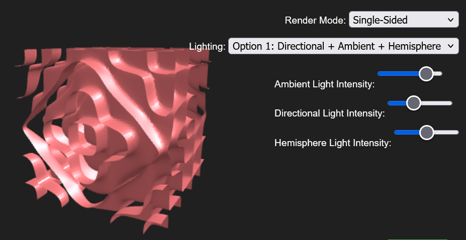
Through the above formulation and cube marching techniques, our group created two open source web versions. A shadertoy implementation as well as a 3js implementation.
Source code and weblinks to both implementations can be seen here.
Image 1: A screenshot of the rendering along with some of the options a user can modify
References
[1] Skrodzki, M., Reitebuch, U., & Polthier, K. (2016). Chladni Figures Revisited: A peek into the third dimension. Proceedings of Bridges 2016: Mathematics, Music, Art, Architecture, Education, Culture, 481–484. http://www.archive.bridgesmathart.org/2016/bridges2016-481.html
This blog was written by Sachin Kishan, Nicolas Pigadas and Bethlehem Tassew during the SGI 2024 Fellowship as one of the outcomes of a one week project under the mentorship of Martin Skrodzki and support of Alberto Tono as teaching assistant.
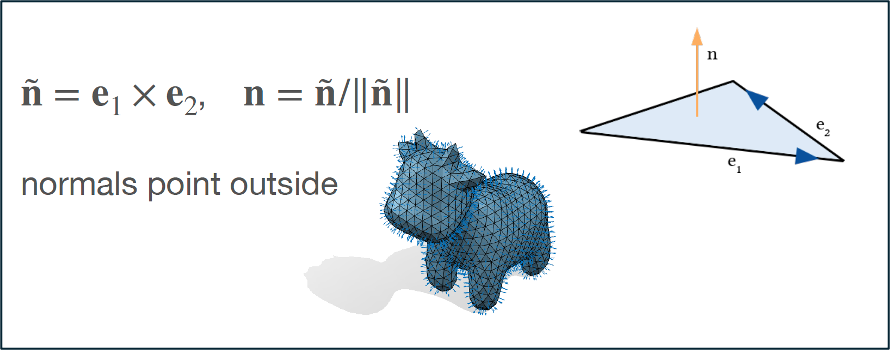
Early in the very first day of SGI, during professor Oded Stein’s great teaching sprint of the SGI introduction in Geometry Processing, we came across normal vectors. As per his slides: “The normal vector is the unit-length perpendicular vector to a triangle and positively oriented”.
Image 1: The formulas and visualisations of normal vectors in professor Oded Stein’s slides.
Immediately afterwards, we discussed that smooth surfaces have normals at every point, but as we deal with meshes, it is often useful to define per-vertex normals, apart from the well defined per-face normals. So, to approximate normals at vertices, we can average the per-face normals of the adjacent faces. This is the trivial approach. Then, the question that arises is: Going a step further, what could we do? We can introduce weights:
Image 2: Introducing weights to per-vertex normal vector calculation instead of just averaging the per-face normals. (image credits: professor Oded Stein’s slides)
How could we calculate them? The three most common approaches are:
1) The trivial approach: uniform weighting wf = 1 (averaging)
2) area weighting wf = Af
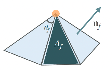
3) angle weighting wf = θf
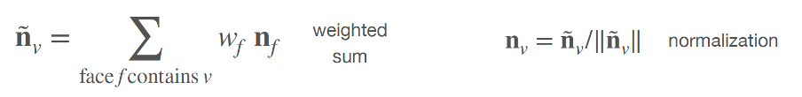
Image 3: The three most common approaches to calculating weights to perform weighted average of the per-face normals for the calculation of per-vertex normals. (image credits: professor Oded Stein’s slides)
During the talk, we briefly discussed the practical side of choosing among the various types of weights and that area weighting is good enough for most applications and, thus, this is the one implemented in gpytoolbox, a Geometry Processing python package that professor Oded Stein has significantly contributed to its development. Then, he gave us an open challenge: whoever was up for the challenge could implement the angle-weighted per-vertex normal calculation and contribute it to gpytoolbox! I was intrigued and below I give an overview of my implementation of the per_vertex_normals(V, F, weights=’area’, correct_invalid_normals=True) function.
Implementation Overview
First, I implemented an auxiliary function called compute_angles(V,F). This function calculates the angles of each face using the dot product between vectors formed by the vertices of each triangle. The angles are then calculated using the arccosine of the dot product cosine result. The steps are:
For each triangle, the vertices A, B, and C are extracted.
Vectors representing the edges of each triangle are calculated:
AB=B−A
AC=C−A
BC=C−B
CA=A−C
BA=A−B
CB=B−C
The cosine of each angle is computed using the dot product:
cos(α) = (AB AC)/(|AB| |AC|)
cos(β) = (BC BA)/(|BC| |BA|)
cos(γ) = (CA CB)/(|CA| |CB|)
At this point, the numerical issues that can come up in geometry processing applications that we discussed on day 5 with Dr. Nicholas Sharp came to mind. What if the values of arccos(angle) exceed the values 1 or -1? To avoid potential numerical problems I clipped the results to be between -1 and 1:
α=arccos(clip(cos(α),−1,1))
β=arccos(clip(cos(β),−1,1))
γ=arccos(clip(cos(γ),−1,1))
Having compute_angles, now we can explore the per_vertex_normals function. It is modified to get an argument to select weights among the options: “uniform”, “angle”, “area” and applies the selected weight averaging of the per-face normals, to calculate the per-vertex normals:
Make sure that the V and F data structures are of types float64 and int32 respectively, to make our function compatible with any given input
Calculate the per face normals using gpytoolbox
If the selected weight is “area”, then use the already implemented function.
If the selected weight is “angle”:
Compute angles using the compute_angles auxiliary function
Weigh the face normals by the angles at each vertex (weighted normals)
Calculate the norms of the weighted normals
(A small parenthesis: The initial implementation of the function implemented the 2 following steps:
Include another check for potential numerical issues, replacing very small values of norms that may have been rounded to 0, with a very small number, using NumPy (np.finfo(float).eps)
Normalize the vertex normals: N = weighted_normals / norms
Can you guess the problem of this approach?*)
6. Identify indices with problematic norms (NaN, inf, negative, zero)
7. Identify the rest of the indices (of valid norms)
8. Normalize valid normals
9. If correct_invalid_normals == True
Build KDTree using only valid vertices
For every problematic index:
Find the nearest valid normal in the KDTree
Assign the nearest valid normal to the current problematic normal
Else assign a default normal ([1, 0, 0]) (in the extreme case no valid norms are calculated)
Normalise the replaced problematic normals
10. Else ignore the problematic normals and just output the valid normalised weighted normals
*Spoiler alert: The problem of the approach was that -in extreme cases- it can happen that the result of the normalization procedure does not have unit norm. The final steps that follow ensure that the per-vertex normals that this function outputs always have norm 1.
Testing
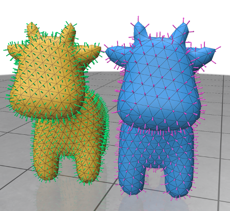
A crucial stage of developing any type of software is testing it. In this section, I provide the visualised results of the angle-weighted per-vertex normal calculations for base and edge cases, as well as everyone’s favourite shape: spot the cow:
Image 4: Let’s start with spot the cow, who we all love. On the left, we have the per-face normals calculated via gpytoolbox and on the right, we have the angle-weighted per-vertex normals, calculated as analysed in the previous section.
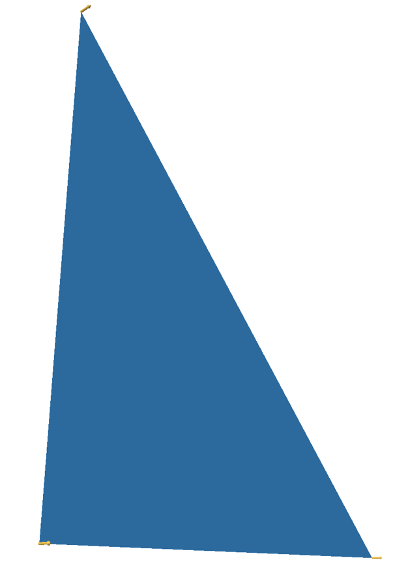
Image 5: The base case of a simple triangle.
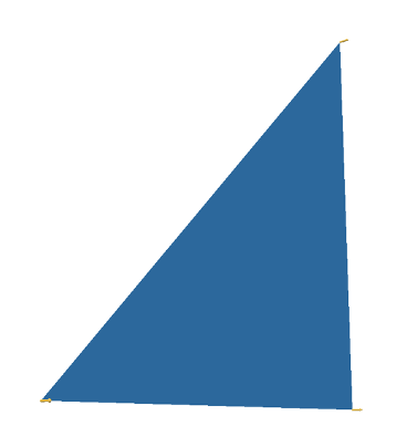
Image 6: The base case of an inverted triangle (vertices ordered in a clockwise direction)
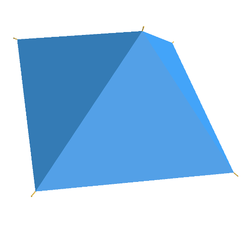
Image 7: The base case of a simple pyramid with a base.
Image 8: The base case of disconnected triangles.
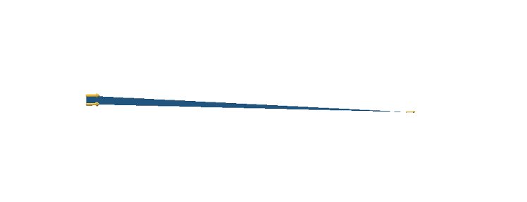
Image 9: The edge case of having a very thin triangle.
Finally, for the cases of a degenerate triangle and repeated vertex coordinates nothing is visualised. The edge cases of having very large or small coordinates have also been tested successfully (coordinates of magnitude 1e8 and 1e-12, respectively).
Having a verified visual inspection is -of course- not enough. The calculations need to be compared to ground truth data in the context of unit tests. To this end, I calculated the ground truth data via the sibling of gpytoolbox: gptoolbox, which is the respective Geometry Processing package but in MATLAB! The shape used to assert the correctness of our per_vertex_normals function, was the famous armadillo. Tests passed for both angle and uniform weights, hurray!
Final Notes
Developing the weighted per-vertex normal function and contributing slightly to such a powerful python library as gpytoolbox, was a cool and humbling experience. Hope the pull request results into a merge! I want to thank professor Oded Stein for the encouragement to take up on the task, as well as reviewing it along with the soon-to-be professor Silvia Sellán!
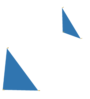
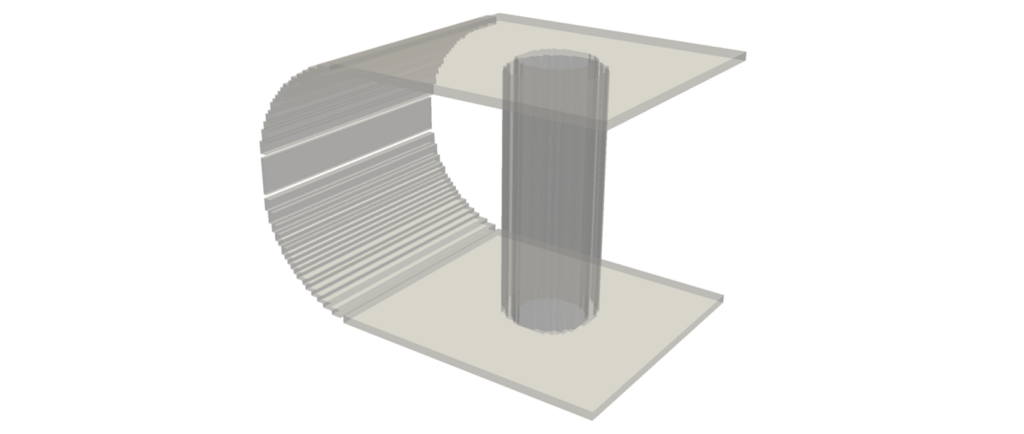
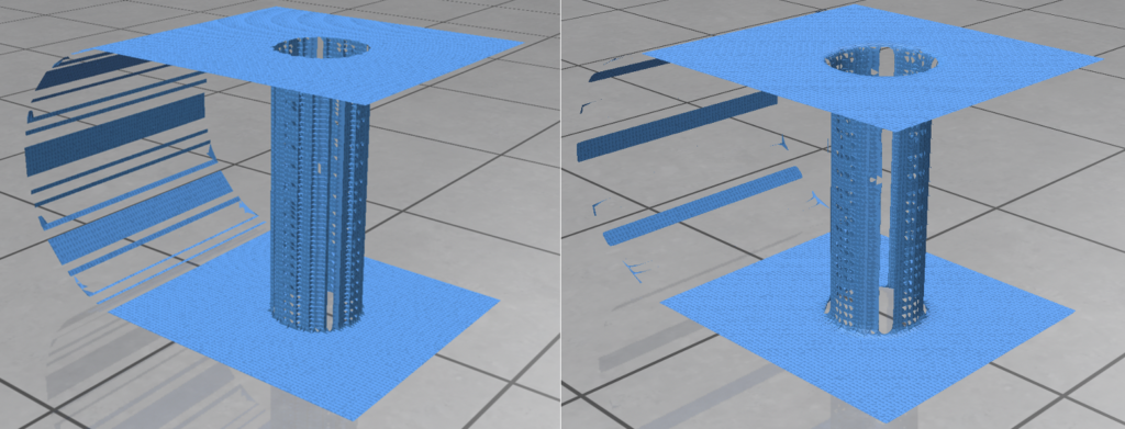
Images: (1) The Wormhole Distance Field (DF) shape. (2) The Wormhole built using DF functions, visualized using a DF/scalar field defined over a discretized space, i.e. a grid. (3) Deploying the marching cubes algorithm (https://dl.acm.org/doi/10.1145/37402.37422) to attempt to reconstruct the surface from the DF shape. (4) Resulting surface using my reconstruction algorithm based on the principles of k-nearest neighbors (kNN), for k=10. (5) Same, but from a different perspective highlighting unreconstructed areas, due to the DF shape having empty areas in the curved plane (see image 2 closely). If those areas didn’t exist in the DF shape, the reconstruction would have likely been exact with smaller k, and thus the representation would have been cleaner and more suitable for ML and GP tasks. (6) The reconstruction for k=5. (7) The reconstruction for k=5, different perspective.
Note: We could use a directional approach to knn for a cleaner reconstructed mesh, leveraging positional information. Alternatively, we could develop a connection correcting algorithm. Irrespectively to if we attempt the aforementioned optimizations or not, we can make the current implementation more optimized, as a lot less distances would need to be calculated after we organize the points of the DF shape based on their positions in the 3D space.
Intro
Well, SGI day 3 came… And it changed everything. In my mind at least. Silvia Sellán and Towaki Takikawa taught us -in the coolest and most intuitive ways- that there is so much more to shape representations. With Silvia, we discussed how one would expect to jump from one representation to another or even try to reconstruct the original shapes from representations that do not explicitely save connectivity information. With Towaki, we discussed Signed Distance Field (SDF) shapes among other stuff (shout out for building a library called haipera, that will definetely be useful to me) and the crazy community building crazy shapes using them. All the newfound knowledge got me thinking. Again.
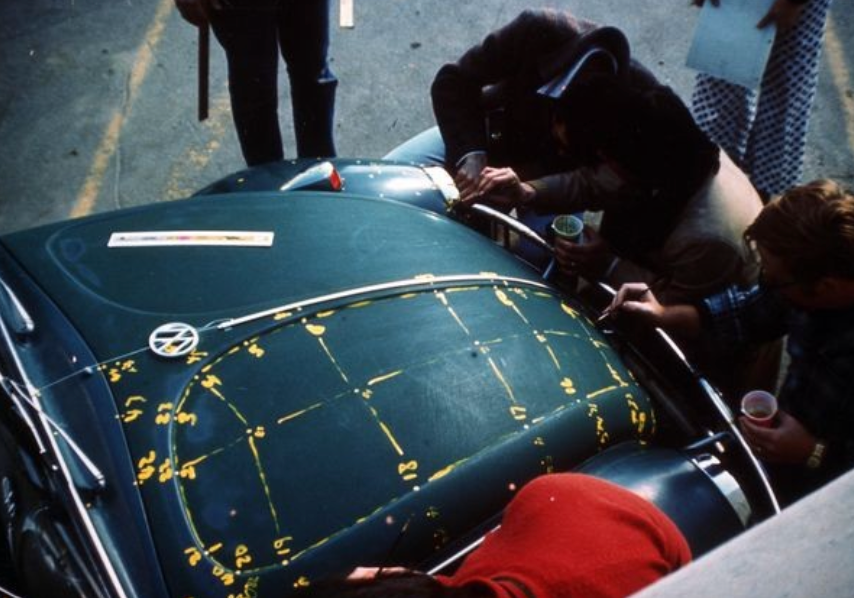
Towaki was asked if there are easier/automated ways to calculate the necessary SDF functions because it would be insane to build -for e.g.- SDF cars by hand. His response? These people are actually insane! And I wanted to get a glimpse of that insanity, to figure out how to build the wormhole using Distance Field (DF) functions. Of course, my target final shape is a lot easier and it turned out that the implementation was far easier than calculating vertices and faces manually (see Wormhole I)! Then, Silvia’s words came to mind: each representation is suitable for different tasks, i.e., a task that is trivial for DF representations might be next to impossible for other representasions. So, creating a DF car is insane, but using functions to calculate the coordinates of a mesh grid car would be even more insane! Fun fact from Silvia’s slides: “The first real object ever 3D scanned and rendered was a WV Beetle by the legendary graphics researcher Ivan Sutherland’s lab (and the car belonged to his wife!)” and it was done manually:
Image (8): Calculating the coordinates of vertices and the faces to design the mesh of a Beetle manually! Geometric Processing gurus’ old school hobbies.
Method
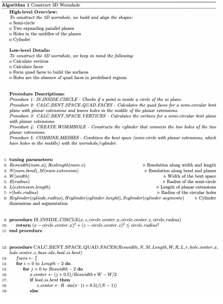
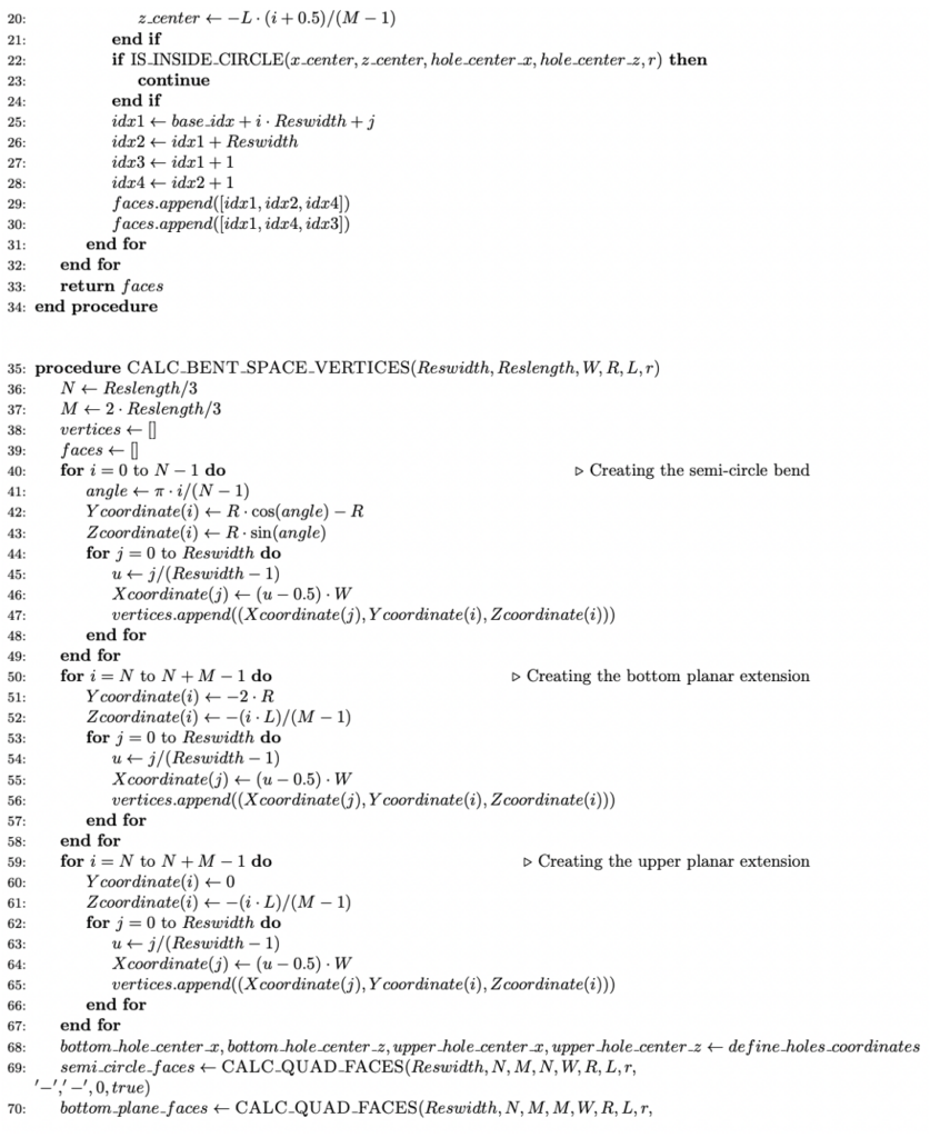
Back to the DF Wormhole. The high-level algorithm for the DF Wormhole is attached below (for the implementation, visit this GitHub repo:
Having my DF Wormhole, the problem of surface reconstruction arose. Thankfully, Silvia had already made sure we got, not only an intuitive understanding of multiple shape representations in 2D and 3D, but also how to jump from one to another and how to reconstruct surfaces from discretized representations. It intrigued me what would happen if I used the marching cubes algorithm on my DF shape. The result was somewhat disappointing (see image 3).
Yet, I couldn’t just let it go. I had to figure out something better. I followed the first idea that came to mind: k-Neirest Neighbors (kNN). My hypothesis was that although the DF shape is in 3D, it doesn’t have any volumetric data. The hypothetical final shape is comprised by surfaces so kNN makes sense; the goal is to find the nearest neighbors and create a mechanism to connect them. It worked (see images 4, 5, 6, 7)! A problem became immediately apparent: the surface was not smooth in certain areas, but rather blocky. Thus, I developed an iterative smoothing mechanism that repositions the nodes based on the average of the coordinates of their neighbors. At 5 iterations the result was satisfying (see image 8). Below I attach the algorithm, (for the implementation, visit this GitHub repo:https://github.com/NIcolasp14/MIT_SGI-Wormhole). Case closed.
Q&A
Q: Why did I call my functions Distance Field functions (DFs) and not Signed Distance Field functions (SDFs)?
A: Because the SDF representation requires some points to have a negative value in relation to a shape’s surface (i.e., we have a negative sign for points inside the shape). In the case of the hollow shapes, such as the hollow cube and cylinder, we replace the negative signs of the inner parts of the outer shapes with positive signs, via the statement max(outer_shape, -inner_shape). Thus, our surfaces/hollow shapes only have 0 values on the surface and positive elsewhere. These type of distance fields are called unsigned (UDFs).
Q: What about the semi-cylinder?
A: The final shape of the semi-cylinder was defined to have negative values inside the radius of the semi-cylinder, 0 on the surface and positive elsewhere. But in order to remove the caps, rather than subtracting an inner cylinder, I gave them a positive value (e.g. infinity). This contradicts the definition of SDFs and UDFs, which measure distance in a continuous way. So, the semi-cylinder would be referred to as a discontinuous distance function (or continuous with specific discontinuities by design).
Future considerations
Using the smoothing mechanism and not using it has a trade off. The smooting mechanism seems to remove more faces -that we do want to have in our mesh-, than if we do not use it (see images 9, 10). The quality of the final surface certaintly depends on the initial DF shape (which indeed had empty spaces, see image 2 closely) and the hyperparameter k of kNN. Someone would need to find the right balance between the aforementioned parameters and the smoothing mechanism or even reconsider how to create the initial Wormhole DF shape or/and how to reposition the vertices, in order to smooth the surfaces more effectively. Finally, all the procedures of the algorithm can be optimized to make the code faster and more efficient. Even the kNN algorithm can be optimized: not every pair must be calculated to compare distances, because we have positional information and thus we can avoid most of the kNN calculations.
Images: (9) Mesh grid using only the mechanism that connects the k-nearest neighbors for k=5, (10) Mesh grid after the additional use of the smoothing mechanism.
This is the 2nd part of the two-part post series, prepared by Krishna and I. Krishna presented an overview of SLAM systems in a very intuitive and engaging way. In this part, I explore the future of SLAM systems in endoscopy and how our team plans to shape it.
Collaborators: Krishna Chebolu
Introduction
What about the future of SLAM endoscopy systems? To get an insight on where research is heading, we must first discuss the challenges posed by the task to localise an agent and map such a difficult environment, as well as the weaknesses of current systems.
On one hand, the environment of the inside of the human body, coupled with data/device heterogeneity and image quality issues, significantly hinder the performance of endoscopy SLAM systems [1], [2] due to:
1) Texture scarceness, scale ambiguity
2) Illumination variation
3) Bodies (foreign or not), fluids and their movement (e.g., mucus, mucosal movement)
6) Underlining scene dynamics (e.g., imminent corruption of frames with severe artefacts, large organ motion and surface drifts)
7) Data heterogeneity (e.g., population diversity, rare or inconspicuous disease cases, variability in disease appearances from one organ to the other, endoscope variability)
8) Difference in device manufacturers
9) Input of experts being required for their reliable development
10) The organ preparation process
11) Additional imaging quality issues (e.g. free/non-uniform hand motions and organ movements, different image modalities)
12) Real time performance (speed and accuracy trade-off)
Current research of endoscopic SLAM systems mainly focuses on the first 3 of the aforementioned challenges; the state-of-the-art pipelines focus on understanding depth despite the lack of texture, as well as handling lighting changes and foreign bodies like mucus that can be reflective or move and, thus, skew the mapping reconstruction.
Images 1, 2, 3: The images above showcase the three main problems that skew the tissue structure understanding and hinder the performance of mapping of SLAM systems in endoscopy: (1) foreign bodies that are reflective (2) lighting variations and (3) lack of texture. Image credits: [3], [3], [4].
On the other hand, we must pinpoint where the weaknesses of such systems lie. The three main modules of AI endoscopy systems, that operate on image data, are Simultaneous Localization and Mapping (SLAM), Depth Estimation (DE) and Visual Odometry (VO); with the last two being submodules of the broader SLAM systems. SLAM is a computational method that enables a device to map its environment while simultaneously determining its own position within that map, which is often achieved via VO; a technique that estimates the camera’s position and trajectory by examining changes across a series of images. Depth estimation is the process of determining the distance between a camera and the objects in its view by analyzing visual information from one or more images, which is crucial for SLAM to accurately map the environment in three dimensions and understand its surroundings more effectively. Attempting to use general purpose SLAM systems on endoscopy data clearly shows that DE and map reconstruction are underperforming, while localisation/VO is sufficiently captured. This conclusion was reached based on initial experiments; however, further investigations are warranted.
Though the challenges and system weaknesses that current research aims to address are critical aspects of the models’ usability and performance, there is still a wide gap between the curated settings under which these models perform and real-world clinical settings. Clinical applications are still uncommon, due to the lack of holistic and representative datasets, in conjuction with limited participation of clinical experts. This leads to models that lack generalisability; widely used supervised techniques are data voracious and require many human annotations, which, apart from scarce, are often imperfect or overfitted to predominant samples in cohorts. Novel deep learning methods should be steered towards training on diverse endoscopic datasets, the introduction of explainability of results and the interpretability of models, which are required to accelerate this field. Finally, suitable evaluation metrics (i.e. generalisability assessments and robustness tests) should be defined to determine the strength of developed methods in regards to clinical translation.
For a future of advanced and applicable AI endoscopy systems, the directions are clear, as discussed in [1]:
1) Endoscopy-specific solutions must be developed, rather than just applying pipelines from the computer vision field
2) Robustness and generalisation evaluation metrics of the developed solutions must be defined to set the standard to assess and compare model performance
3) Practicability, compactness and real time effectiveness should also be quantified
4) More challenging problems should be explored (subtle lesions instead of apparent lesions)
5) The developed models should be able to adapt to datasets produced in different clinics, using different endoscopes, in the context of varying manifestations of diseases
6) Multi-modal and multi-scale integration of data should be incorporated in these systems
7) Clinical validation is necessary to steadily integrate these systems in the clinical process
Method
But how do weenvision the future of SLAM endoscopy systems?
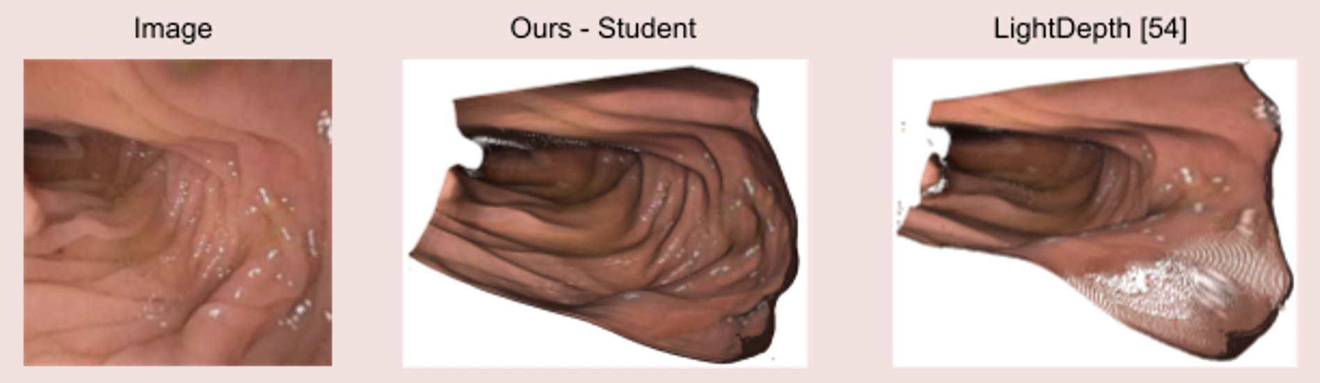
Our team aims to address directly the issues of texture scarceness, illumination variation and handling of foreign bodies, while indirectly combating some of the rest of the challenges. Building upon state-of-the-art SLAM systems, which already handle localisation/VO sufficiently, we aim to further enhance their mapping process, by integrating a state-of-the-art endoscopy monocular depth estimation pipeline [3] and by developing a module to understand lighting variations in the context of endoscopic image analysis. The aforementioned module will have a corrective nature, automatically adjusting the lighting in the captured images to ensure that the visuals are clear and consistent. Potentially, it could also enhance the image quality by adjusting brightness, contrast, and other image parameters in real-time, standardizing the images of different frames of the endoscopy video. As the module’s task is to improve the visibility and consistency of the image features, it would consequentially also support the depth estimation process, by providing clearer cues and contrast for accurate depth calculations by the endoscopy monocular depth estimation pipeline. Thus, the module would ensure a more consistent and refined input to the SLAM model, rather than raw endoscopy data, which suffer from inconsistencies and heterogeneities, never seen before by the model. With the aforementioned integrations we aim to develop a specialised SLAM endoscopy system and test it in the context of clinical colonoscopy [5]. Ideally, the plan is to first train and test our pipeline on a curated dataset to test its performance under controlled settings and then it would be of great interest to adjust each part of the pipeline to make it perform on real-world clinical data or across multiple datasets. This will provide us with the opportunity to see where a state-of-the-art SLAM endoscopy system stands in the context of real-world applicability and help quantify and address the issues explored in the previous section.
Image 4: State-of-the-art clinical mesh reconstruction using the endoscopy monocular depth estimation pipeline [5].
Image 5: The endoscopy monocular depth estimation pipeline also extracts state-of-the-art depth estimation in endoscopy videos.
Colonoscopy Data
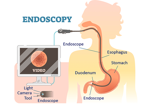
The type of endoscopy procedure we choose to develop our pipeline for is colonoscopy; a medical procedure that uses a flexible fibre-optic instrument equipped with a camera and light (a colonoscope) to examine the interior of the colon and rectum. More specifically, we select to work with the Colonoscopy 3D Video Dataset (C3VD) [5]. The significance of this dataset study is the fact that it provides high quality ground truth data, obtained using a high-definition clinical colonoscope and high-fidelity colon models, creating a benchmark for computer vision pipelines. The study introduced a novel multimodal 2D-3D registration technique to register optical video sequences with ground truth rendered views of a known 3D model.
Video 1: C3VD dataset: Data from the colonoscopy camera (left) and depth estimation (right) extracted by a Generative Adversarial Network (GAN). Video credits: [5]
Conclusion
SLAM systems are the state-of-the-art for localisation and mapping and endoscopy is the gold standard procedure for many hollow organs. Combining the two, we get a powerful medical tool that can not only improve patient care, but also be life-defining in some cases. Its use cases can be prognostic, diagnostic, monitoring and even therapeutic, ranging from, but not limited to: disease surveillance, inflammation monitoring, early cancer detection, tumour characterisation, resection procedures, minimally invasive treatment interventions and therapeutic response monitoring. With the development of SLAM endoscopy systems, the endoscopy surgeon has acquired a visual overview of various environments inside the human body, that would otherwise be impossible. Endoscopy being highly operator-dependent with grim clinical outcomes in some disease cases, makes reliable and accurate automated system guidance imperative. Thus, in recent years, there has been a significant increase in the publication of endoscopic imaging-based methods within the fields of computer-aided detection (CADe), computer-aided diagnosis (CADx) and computer-assisted surgery (CAS). In the future, most designed methods must be more generalisable to unseen noisy data, patient population variability and variable disease appearances, giving an answer to the multi-faceted challenges that the latest models fail to address, under actual clinical settings.
This post concludes part 11 of What it Takes to Get a SLAM Dunk.
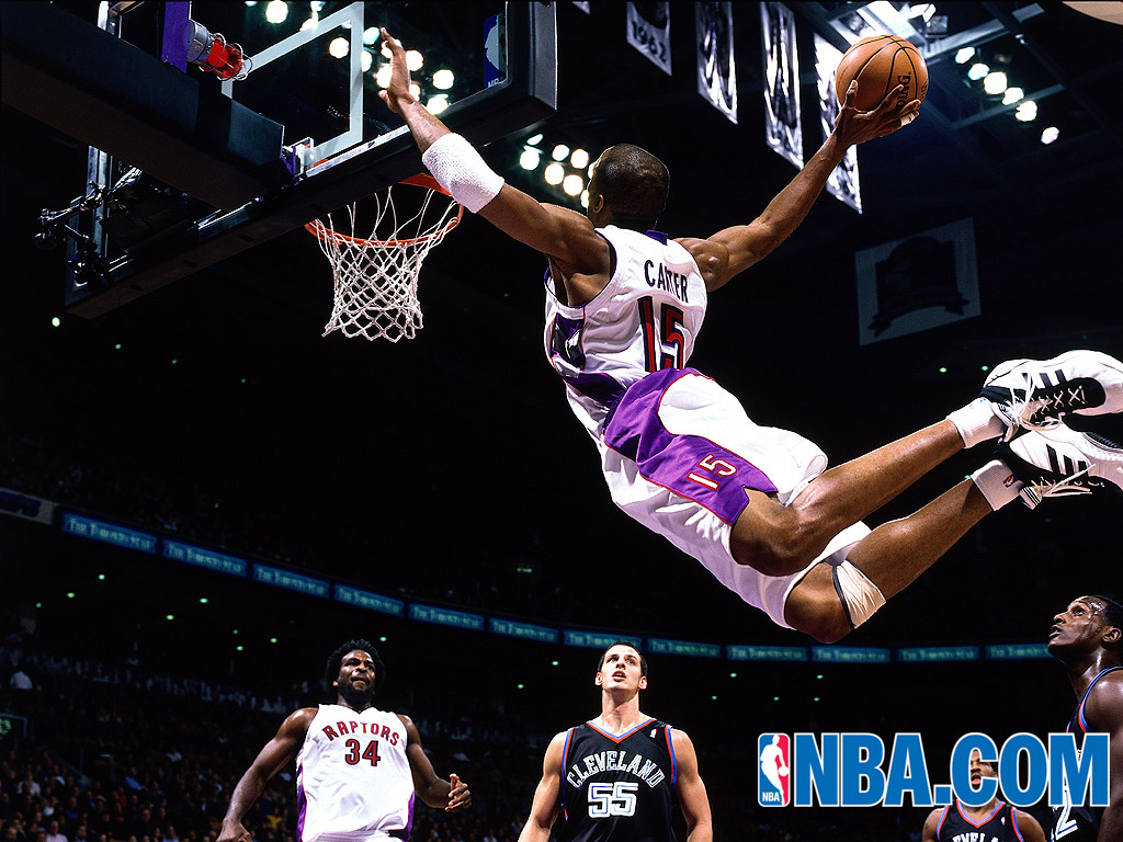
Image 6: Michael Jordan (considered by me and many as the G.O.A.T.) performing his most famous dunk. Image credits: ScienceABC
References
[1] Ali, S. Where do we stand in AI for endoscopic image analysis? Deciphering gaps and future directions. npj Digit. Med.5, 184 (2022). https://doi.org/10.1038/s41746-022-00733-3
[2] Ali, S., Zhou, F., Braden, B. et al. An objective comparison of detection and segmentation algorithms for artefacts in clinical endoscopy. Sci Rep10, 2748 (2020). https://doi.org/10.1038/s41598-020-59413-5
[3] Paruchuri, A., Ehrenstein, S., Wang, S., Fried, I., Pizer, S. M., Niethammer, M., & Sengupta, R. Leveraging near-field lighting for monocular depth estimation from endoscopy videos. In Proceedings of the European Conference on Computer Vision (ECCV), (2024). https://doi.org/10.48550/arXiv.2403.17915
[5] Bobrow, T. L., Golhar, M., Vijayan, R., Akshintala, V. S., Garcia, J. R., & Durr, N. J. Colonoscopy 3D video dataset with paired depth from 2D-3D registration. Medical Image Analysis, 102956 (2023). https://doi.org/10.48550/arXiv.2206.08903
In this two-part post series, Nicolas and I dive deeper into SLAM systems– our project’s focus for the past two weeks. In this part, I introduce and cover the evolution of SLAM systems. In the next part, Nicolas harnesses our interest by discussing the future. By the end of both parts, we should be able to give you an overview of What it Takes to Get a SLAM Dunk.
Collaborators: Nicolas Pigadas
Introduction
Simultaneous Localization and Mapping (SLAM) systems have become a standard in various technological fields, from autonomous robotics to augmented reality. However, in recent years, this technology has found a particularly unique application in medical imaging– in endoscopic videos. But what is SLAM?
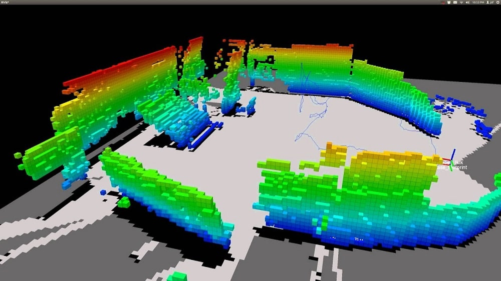
Figure 1: A sample image using SLAM reconstruction from SG News Desk.
SLAM systems were conceptualized in robotics and computer vision for navigation purposes. Before SLAM, the fields employed more elementary methods,
Mapping: the process of creating a representation of an environment, typically in the form of a 2D or 3D map. This was done using grid-based and feature-based methods.
You may be thinking, Krishna, you just described SLAM systems, it sounds like. You are right, but the localizing and mapping were separate processes. So a robot would go through the pains of the Heisenberg principle, i.e., the robot would either localize or map– the or is exclusionary.
It was fairly obvious, but still daunting what the next step in research would be. Before we SLAM dunk our basketball, we must do a few lay-ups and free-throw shoots first.
Precursors to SLAM
Here are some inspirations that contributed to the development of SLAM
Probabilistic robotics: The introduction of probabilistic approaches, such as Bayesian filtering, allowed robots to estimate their position and map the environment with a degree of uncertainty, paving the way for more integrated systems.
Kalman filtering: a mathematical technique for estimating the state of a dynamic system. It allowed for continuous estimation of a robot’s position and could be invariant to noisy sensor data.
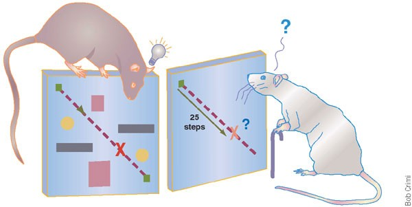
Cognitive Mapping in Animals: Research in cognitive science and animal navigation provided theoretical inspiration, particularly the idea that animals build mental maps of their environment while simultaneously keeping track of their location.
Figure 3: Spatial behavior and cognitive mapping of mice with aging. Image from Nature.
SLAM Dunk – A Culmination (some real Vince Carter stuff)
Finally, many researchers agreed that the separation of localizing and mapping was ineffective, and great efforts went into their integration. SLAM was developed. The goal was to enable systems to explore and understand an unknown environment autonomously, they needed to localize and map the environment simultaneously, with each task informing and improving the other.
With its unique ability to localize and map, researchers found SLAM’s use in any sensory device. Some of SLAM’s earlier use were sensor-based; so data would be inputted from range finders, sonar, and LIDAR; in the late 80s and early 90s. It is good to note that the algorithms were computationally intensive– and still are.
As technology evolved, a vision-based SLAM emerged. This shift was inspired by the human visual system, which navigates the world primarily through sight, enabling more natural and flexible mapping techniques.
Key Milestones
With the latest iterations of SLAM being exponentially better than the origin, it is important to recognize the journey. Here are notable SLAM systems:
EKF-SLAM (Extended Kalman Filter SLAM): One of the earliest and most influential SLAM algorithms, EKF-SLAM, laid the foundation for probabilistic approaches to SLAM, allowing for more accurate mapping and localization.
FastSLAM: Introduced in the early 2000s, FastSLAM utilized particle filters, making it more efficient and scalable. This development was crucial in enabling real-time SLAM applications.
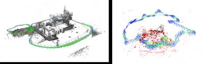
Visual SLAM: The transition to vision-based SLAM in the mid-2000s opened new possibilities for the technology. Visual SLAM systems, such as PTAM (Parallel Tracking and Mapping), enabled more detailed and accurate mapping using standard cameras, a significant step toward broader applications.
Figure 4: Left LSD-SLAM, right ORB-SLAM. Image found in fzheng.me
From Robotics to Endoscopy (Medical Vision)
As SLAM technology matured, researchers explored its potential beyond traditional robotics. Medical imaging, particularly endoscopy, presented a fantastic opportunity for SLAM. Endoscopy is a medical procedure involving a flexible tube with a camera to visualize the body’s interior, often within complex and dynamic environments like the gastrointestinal tract.
It is fairly trivial why SLAM could be applied to endoscopic and endoscopy-like procedures to gain insights and make more medically informed decisions. Early work focused on using visual SLAM to navigate the gastrointestinal tract, where the narrow and deformable environment presented significant challenges.
One of the first successful implementations involved using SLAM to reconstruct 3D maps of the colon during colonoscopy procedures. This approach improved navigation accuracy and provided valuable information for diagnosing conditions like polyps or tumors.
Researchers also explored the integration of SLAM with other technologies, such as optical coherence tomography (OCT) and ultrasound, to enhance the quality of the maps and provide additional layers of information. These efforts laid the groundwork for more advanced SLAM systems capable of handling the complexities of real-time endoscopic navigation.
Figure 6: Visual of Optical Coherence Tomography from News-Medical.
Endoscopy SLAMs – What Our Group Looked At
As a part of our study, we looked at some presently used and state-of-the-art SLAM systems. Below are the three that various members of our team attempted:
NICER-SLAM (RGB): a dense RGB SLAM system that simultaneously optimizes for camera poses and a hierarchical neural implicit map representation, which also allows for high-quality novel view synthesis.
ORB3-SLAM (RBG): (there is also ORB1 and ORB2) ORB-SLAM3 is the first real-time SLAM library able to perform Visual, Visual-Inertial, and Multi-Map SLAM with monocular, stereo, and RGB-D cameras, using pin-hole and fisheye lens models. In all sensor configurations, ORB-SLAM3 is as robust as the best systems available in the literature and significantly more accurate.
DROID-SLAM (RBG): a new deep learning-based SLAM system. DROID-SLAM consists of recurrent iterative updates of camera pose and pixel-wise depth through a Dense Bundle Adjustment layer.
Some other SLAM systems that our team would have loved to try our hand at are:
Gaussian Splatting SLAM: first application of 3D Gaussian Splatting in monocular SLAM, the most fundamental but the hardest setup for Visual SLAM.
GlORIE-SLAM: Globally Optimized RGB-only Implicit Encoding Point Cloud SLAM. This system uses a deformable point cloud as the scene representation and achieves lower trajectory error and higher rendering accuracy compared to competitive approaches.
This concludes part 1 of What it Takes to Get a SLAM Dunk. This post should have given you a gentle, but robust-enough introduction to SLAM systems. Vince Carter might even approve.
Figure 9: An homage to Vince Carter, arguably the greatest dunk-er ever. Image from Bleacher Report.
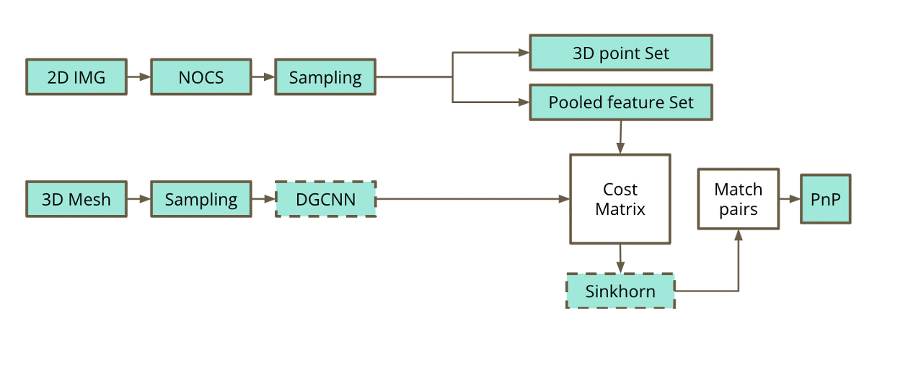
Image 1: Our proposed solution’s pipeline, credits to our -always supportive- mentors, Saleh Mahdi and Dani Velikova!
Introduction
Our project aims to enhance Optimal Transport (OT) solvers by incorporating Graph Neural Networks (GNNs) to address the lack of geometric consistency in feature matching. The main motivation of our study is that a lot of real objects are symmetric and thus impose ambiguity. Traditional OT approaches focus on similarity measures and often neglect important neighboring information in geometric settings, proper in computer vision or graphics problems, resulting in the production of huge noise in pose estimation tasks. To tackle this problem, we hypothetize that when the object is symmetric, there are many correct matches of points around its symmetric axis and we can leverage this fact via Optimal Transport and Graph Learning.
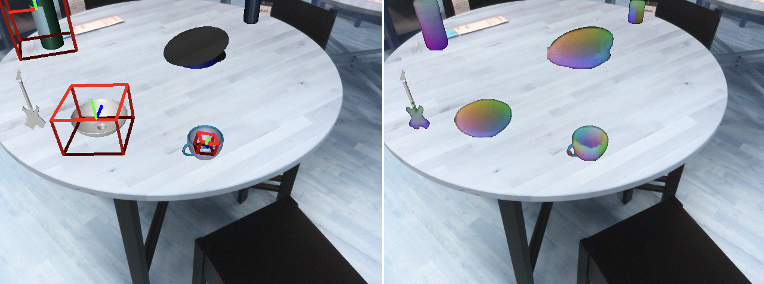
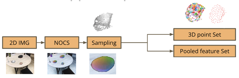
To this end, we propose the pipeline in image 1. On a high level, we extract a 3D point cloud of an object from a 2D scene using the Normalized Object Coordinate Space (NOCs) pipeline [1], downsample the points and pool the features/NOCs embeddings of the removed points into the representative remaining points. Concurrently, we run DGCNN on the 3D ground truth mesh of the object and create a graph; this model is used as a 3D encoder [2]. We combine the aforementioned embeddings into the cost matrix used by the Sinkhorn algorithm [3], which attempts to match the points of the point cloud produced by the NOCs map with the nodes of the graph produced by the DGCNN and then to provide a symmetry estimation. We extend the differentiable Sinkhorn solver to yield one-to-many solutions; a modification we make to fully capture the symmetry of a texture-less object. In the final step, we match pairs of points and pixels and perform symmetric pose estimation via Perspective-n-Point. In this post, we study one part of our proposed pipeline, the extended NOCs, from the 2D image analysis to the extraction of the 3D point set and the pooled feature set.
Extended NOCs pipeline
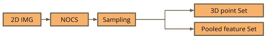
Image 2: The part of the pipeline we will study in this post: Generating a 3D point cloud of a shape from a chosen 2D scene and downsampling its points. We pool the features of the removed points into remaining (seed) points.
The NOCs pipeline extracts the NOCs map and provides size and pose estimation for each object in the scene. The NOCs map encodes via colours the prediction of the normalized 3D coordinates of the target objects’ surfaces within a bounded unit cube. We extend the NOCs pipeline to create a 3D point cloud of the target object using the extracted NOCs map. We then downsample the point cloud, by fragmenting it using the Farthest Point Sampling (FPS) algorithm and only keeping the resulting seed points. In order to fully encapsulate the information extracted by the NOCs pipeline, we pool the embeddings of the nodes of each fragment into the seed points, by averaging them. This enables our pipeline to leverage the features of the target object’s 2D partial view in its scene.
Data
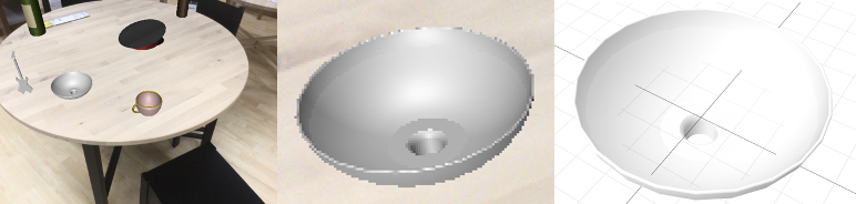
Images 3, 4, 5: (3) The scene of the selected symmetric and texture-less object. (4) The object in the scene zoomed in. (5) The ground truth of the object, i.e. its exact 3D model.
In order to test our hypothesis, we use an object that is not only symmetric, but also texture-less and pattern-free. The specifications of the object we use are the following:
Link to download: https://github.com/sahithchada/NOCS_PyTorch?tab=readme-ov-file
Extended NOCs pipeline: steps visualised
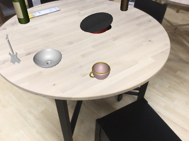
In this section we visually examine each part of the pipeline and how it processes the target shape. First, we get a 2D image of a 3D scene, which is the input of the NOCs pipeline:
Image 6: The 3D scene to be analyzed.
Running the NOCs pipeline on it, we get the pose and size estimation, as well as the NOCs map for every object in the scene:
Image 7, 8: (7) Pose and size estimation of the objects in the scene. (8) NOCs maps of the objects.
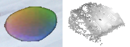
The color encodings in the NOCs map encode the prediction of the normalized 3D coordinates of the target objects’ surfaces, within a bounded a unit cube. We leverage this prediction to reconstruct the 3D point cloud of our target shape, from its 2D representation in the scene. We used a statistical outlier removal method to refine the point cloud and remove noisy points. We got the following result:
Images 9, 10: (9) The 2D NOCs map of the object. (10) The 3D point cloud reconstruction of the 2D NOCs map of the target object.
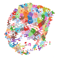
The extracted 3D point cloud of the target object is then fragmented using the Farthest Point Sampling (FPS) algorithm and the seed (center/representative) points of each fragment are also calculated.
Image 11: The fragmented point cloud of the target object. Each fragment contains its corresponding seed point.
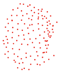
The Sinkhorn algorithm part of our project requires a lot less data points for an optimized performance. Thus, we downsample the 3D point cloud, by only keeping the seed points. In order to capture the information extracted by the NOCs pipeline, we pool the embeddings of the removed features into their corresponding seed points via averaging:
Image 12: The 3D seed point cloud. Into each seed point, we have pooled the embeddings of the removed points of their corresponding fragment.
An overview of each step and the visualised result can be seen below:
Image 13: The scene and object’s visualisation across every step of the pipeline.
Conclusion
In this study, we discussed the information extraction of a 3D object from a 2D scene. In our case, we examined the case of a symmetric object. We downsampled the resulting 3D point cloud in order for it to be effectively handled by later stages of the pipeline, but we made share to encapsulate the features of the removed points via pooling. It will be very interesting to see how every part of the pipeline comes together to predict symmetry!
At this point, I would like to thank our mentors Mahdi Saleh and Dani Velikova, as well as Matheus Araujo for their continuous support and understanding! I started as a complete beginner to these computer vision tasks, but I feel much more confident and intrigued by this domain!
[1] He Wang, Srinath Sridhar, Jingwei Huang, Julien Valentin, Shuran Song, and Leonidas J. Guibas. Normalized object coordinate space for category-level 6d object pose and size estimation, 2019. [2] Yue Wang, Yongbin Sun, Ziwei Liu, Sanjay E. Sarma, Michael M. Bronstein, and Justin M. Solomon. Dynamic graph cnn for learning on point clouds, 2019. [3] Paul-Edouard Sarlin, Daniel DeTone, Tomasz Malisiewicz, and Andrew Rabinovich. Superglue: Learning feature matching with graph neural networks. CoRR, abs/1911.11763, 2019.
Images: (1) Top left: Wormhole built using Python and Polyscope with its triangle mesh, (2) Top right: Wormhole with no mesh, (3) Bottom left: A concept of a wormhole (credits to: BBC Science Focus, https://www.sciencefocus.com/space/what-is-a-wormhole), (4) A cool accident: an uncomfortable restaurant booth.
During the intense educational week that is SGI’s tutorial week, we stumbled early on, on a challenge: creating our own mesh. A seemingly small exercise to teach us to build a simple mesh, turned for me into much more. I always liked open projects that speak to the creativity of students. Creating our own mesh could be turned into anything and our only limit is our imagination. Although the time was restrictive, I couldn’t but face the challenge. But what would I choose? Fun fact about me: in my studies I started as a physicist before I switched to be an electrical and computer engineer. But my fascination for physics has never faded, so when I thought of a wormhole I knew I had to build it.
From Wikipedia: A wormhole is a hypothetical structure connecting disparate points in spacetime and is based on a special solution of the Einstein field equations. A wormhole can be visualised as a tunnel with two ends at separate points in spacetime.
Well, I thought that it would be easier than it really was. It was daunting at first -and during the development I must confess-, but when I started to break the project into steps (first principles thinking), it felt more manageable. Let’s examine the steps on a high level/top-down:
1) build a semi-circle
2) extend its both ends with lines of the same length and parallel to each other
3) make the resulting shape 3D
4) make a hole in the middle of the planes
5) connect the holes via a cylinder
And now let’s explore the bottom-up approach:
1) calculate vertices
2) calculate faces
3) form quad faces to build the surfaces
4) holes are the absence of quad faces in predefined regions
I followed this simple blueprint and the wormhole started to take shape step by step. Instead of giving the details in a never-ending text, I opt to present a high-level algorithm and the GitHub repoof the implementation.
My inspiration for this project? Two-fold; stemming from the very first day of SGI. On one hand, professor Oded Stein encouraged us to be artistic, to create art via Geometry Processing. On the other, Dr. Qingnan Zhou from Adobe shared with us 3 practical tips for us geometry processing newbies:
1) Avoid using background colours, prefer white
2) Use shading
3) Try to become an expert in one of the many tools of Geometry Processing
Well, the third stuck with me, but -of course- I am not close to becoming a master of Python for Geometric Processing and Polyscope, yet. Though, I feel like I made significant strides with this project!
I hope that this work will inspire other students to seek open challenges and creative solutions or even build upon the wormhole, refine it or maybe add a spaceship passing through. Maybe a new SGI tradition? It’s up to you!
P.S. 1: The alignment of the shapes is a little bit overengineered :).
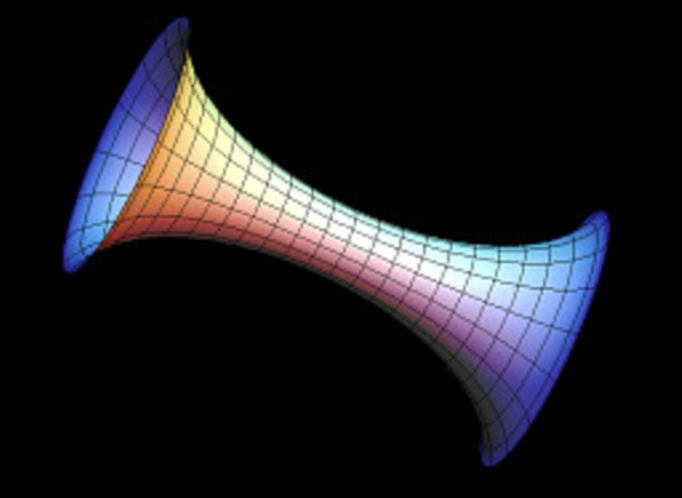
P.S. 2: Unfortunately, it was later in the tutorial week that I was introduced to the 3DXM virtual math museum. Instead of a cylinder, the wormhole should have been a Hyperbolic K=-1 Surface of Revolution, making the shape cleaner: