By Aditya Abhyankar, Biruk Abere, Francisco Unai Caja López and Sara Ansari

Mentored by Kartik Chandra with help from the volunteer Shaimaa Monem

In this project we are looking for ways to generate physical illusions. More to the point, we would like to generate objects that, similarly to this bird, can be balanced in a surprising way with just one support point. To do this we have considered both the physics of the system and we draw on theories from cognitive science to model human intuition.

1. Introduction

Every day in your life, you make thousands of intuitive physical judgements without noticing. ‘Will this pile of dishes in the sink fall if I move this cup?’, ‘If it does fall, in which way will it fall?’ The judgements we make are accurate in most scenarios, but sometimes mistakes happen. Just like how occasional errors in vision lead to visual
illusions (e.g. the dress and the Muller-Lyer illusion) occasional errors in intuitive physics should lead to physical illusions. To generate new illusions, there are two steps that could be followed.

1. First, we could design a method that appropriately models the way people make intuitive judgements based on their perception of the world. In that regard it’s interesting to read [1] which models intuitive physical judgement via physical simulations.
2. Secondly, we could try to ‘fool our model’ or to find an adversarial example. That is, find a physical scenario in which the output of the model is wrong. If the model is appropriately chosen, the results may also fool humans, thus producing new physical illusions. This approach has been used in [2] to generate images with properties similar to the dress.

In this project we aim to find a different kind of illusion. Consider the following toy (image from Amazon). Many people would guess that the bird would fall if it’s only supported by its beak.

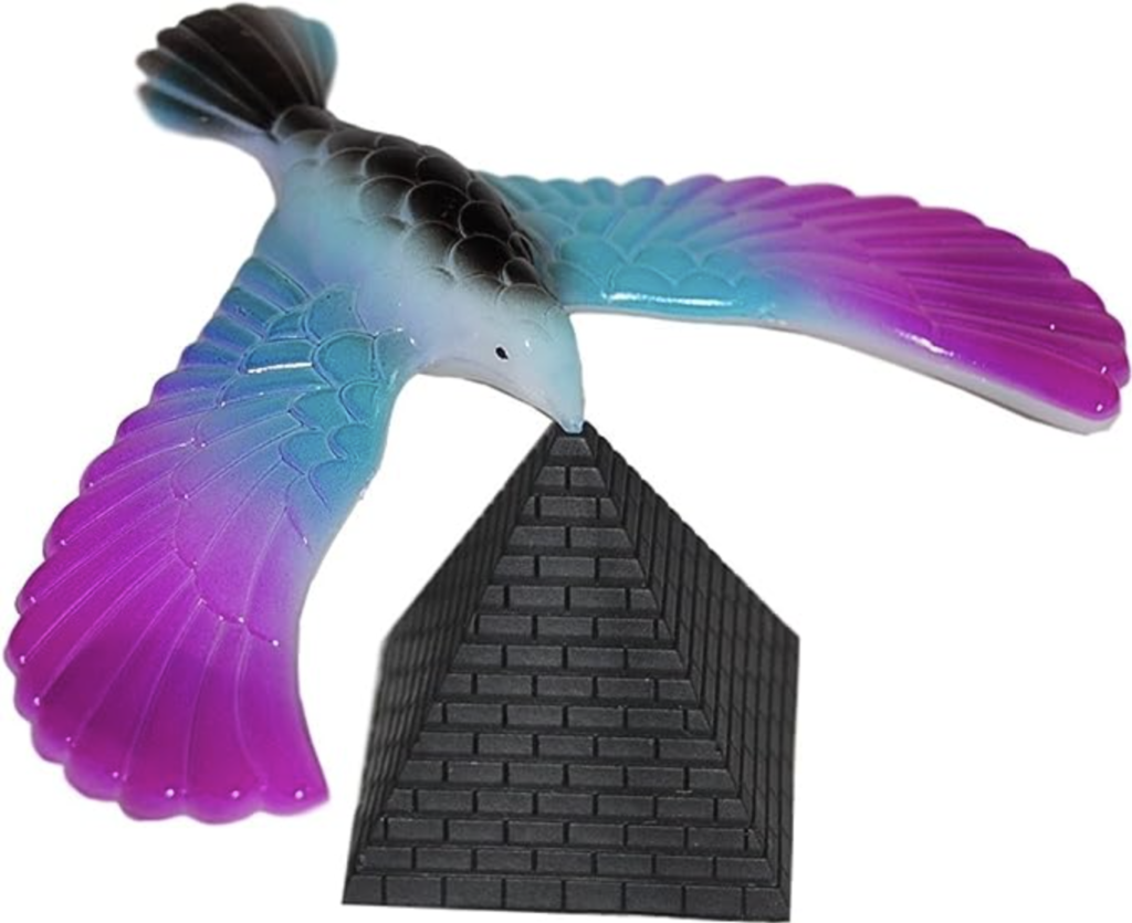
However, the toy achieves a perfectly stable balance in that position. We seek to find other objects that behave similarly: they achieve stable balance given a single support point even when many people guess that it is going to fall.

2. Physical stability vs intuitive stability

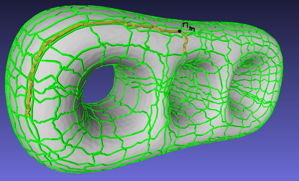
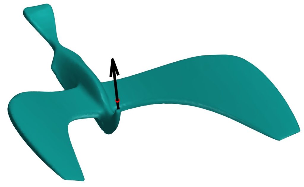
Consider a frictionless rigid body with uniform density and a point p on its boundary with unit normal n. For the object to balance at p, its normal n must point ‘downwards’ in the direction of gravity, for otherwise it will slide. Perfect balancing will then be achieved if the line connecting p and the object’s volumetric center of mass (COM) m is parallel to n. This can be achieved for the balancing bird when the point p is the beak as can be approximately seen in the following figure (mesh obtained from thingiverse). Here we have the center of mass in red and the vector showing the direction of m−p.

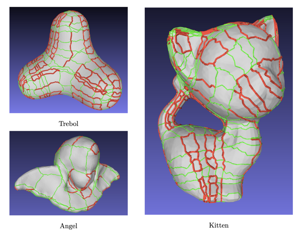
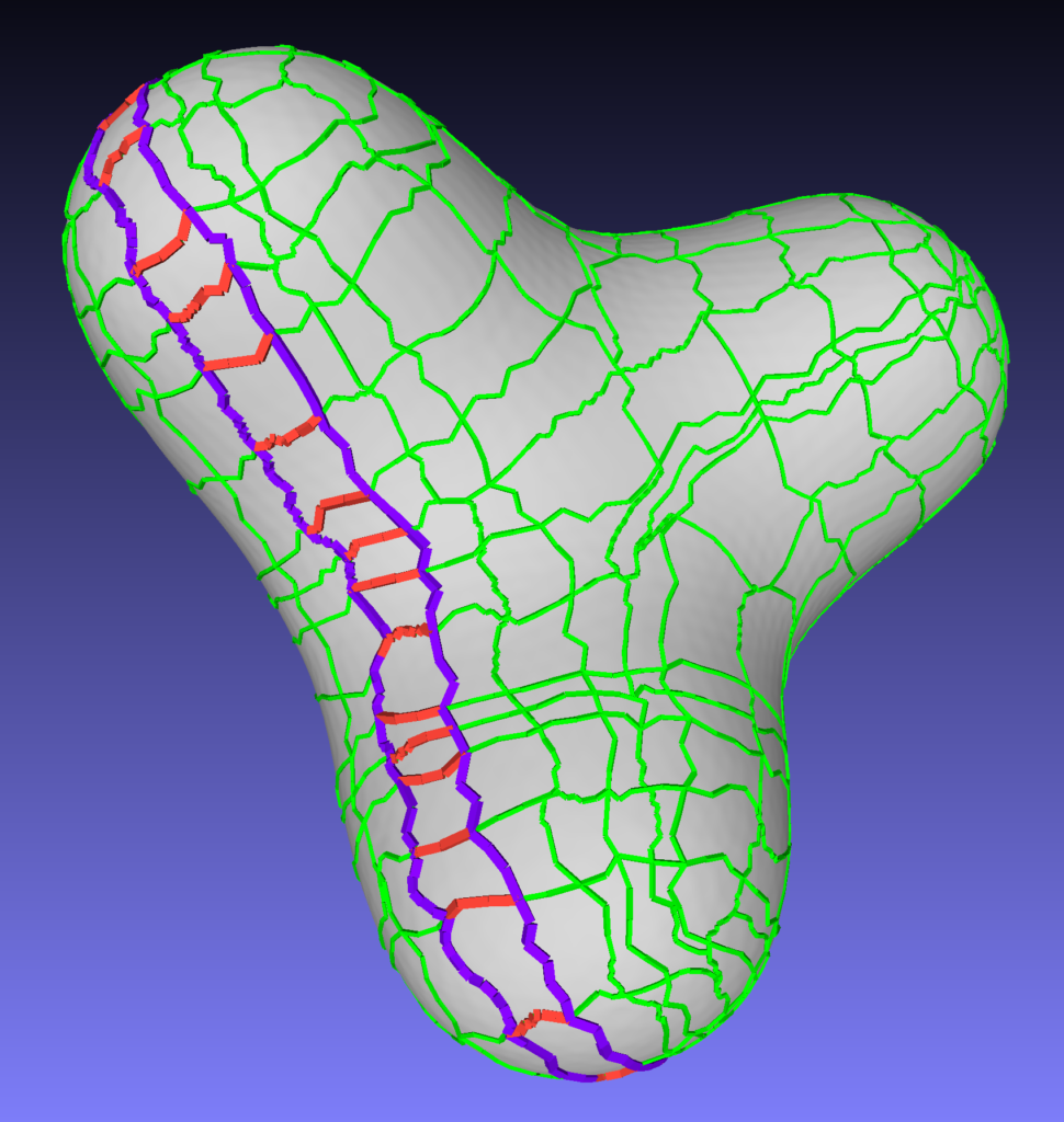
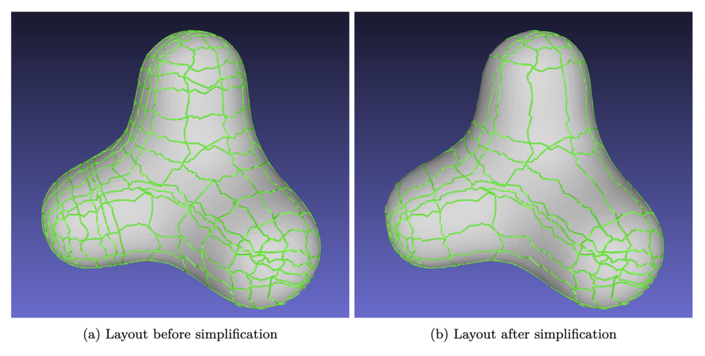
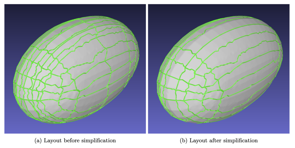
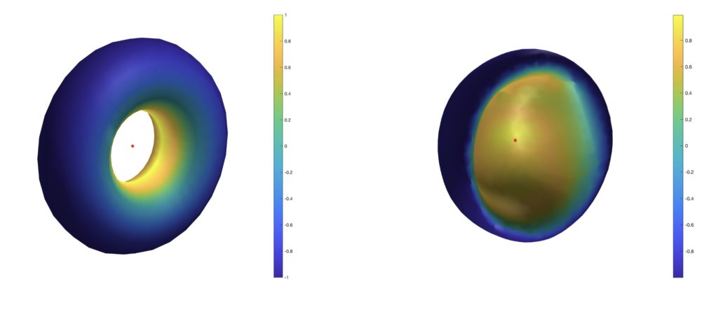
Since an object can always be rotated so that n points downwards, the quality of the balancing can be assessed by the evaluating the dot product (m−p) · n. To be precise, we use the normalized vectors to compute the dot product. The greater this value, the more stable the balancing at p. If m−p and n are parallel and have the same direction, then a perfect balancing will be achieved, and it will be stable. If they are parallel with opposite direction, a perfect balancing will still be achieved, but it will be unstable; i.e. small perturbations will make it fall. Points with dot product values in between will lie somewhere on a spectrum of stability, determined by their dot product’s closeness to the positive extremum. To illustrate this concept, we have taken a torus and a ‘half coconut’ mesh and plotted the dot product of normalized m−p, n. The center of mass appears in red.

There is some evidence [4] that humans asses a rigid body’s ability to stably balance at a point in a very similar way. The only difference is that instead of considering the object’s actual COM, whose location can be counterintuitive even with uniform density, humans judge stability based on the COM m_ch of the object’s convex hull. Thus to find an object that stably balances in a way that looks counterintuitive to humans, we must search for objects with at least one boundary point p such that (m−p) · n is maximized, but (m_ch−p) · n is minimized.

In general, to compute the center of mass of a region M⊂ℝ³, we would need to compute the volume integral

\(\mathbf m=\left(\int_{M}x\rho(x,y,z)\,dxdydz,\int_{M}y\rho(x,y,z)\,dxdydz,\int_{M}z\rho(x,y,z)\,dxdydz\right)\)

where ρ is the density of the object. However, for watertight surfaces with constant density, this volume integral can be turned into a surface integral thanks to Stokes’ theorem. Therefore, the center of mass can be computed even if we only know the boundary of the object, which for us is encoded as a triangle mesh. The interested reader learn more about this computation in [3].

3. Finding new illusions

Given a mesh, one simple way to find new illusions would be to look for a vertex p such that (m−p) · n is positive and close to its maximum, while (m_ch−p) · n is as small as possible (again, we will use normalized versions of the vectors). Of course, these are two conflicting tasks. In this project we have chosen to maximize a function of the form

\(w\frac{(\mathbf m-\mathbf p)\cdot \mathbf n}{\vert \mathbf m-\mathbf p\vert}-\frac{(\mathbf m_{\text{ch}}-\mathbf p)\cdot \mathbf n}{\vert \mathbf m_{\text{ch}}-\mathbf p\vert}\)

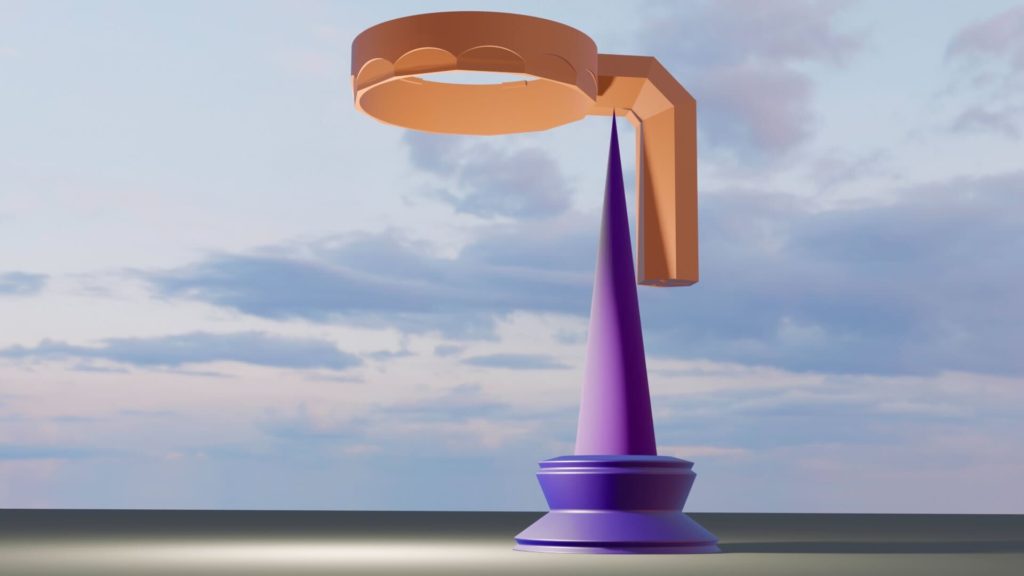
where w is a weight. By increasing w, we are more likely to find points were m−p and n are almost parallel, which is desirable to achieve a stable balance. The most interesting results were found when (m−p) · n ≈ |m−p| and (m_ch−p) · n < 0.7|m_ch−p|. For instance, we have the following chair.

This chair is part of the SHRECK 2017 dataset. We also examined some meshes from Thingi10k and one of the results was the following.

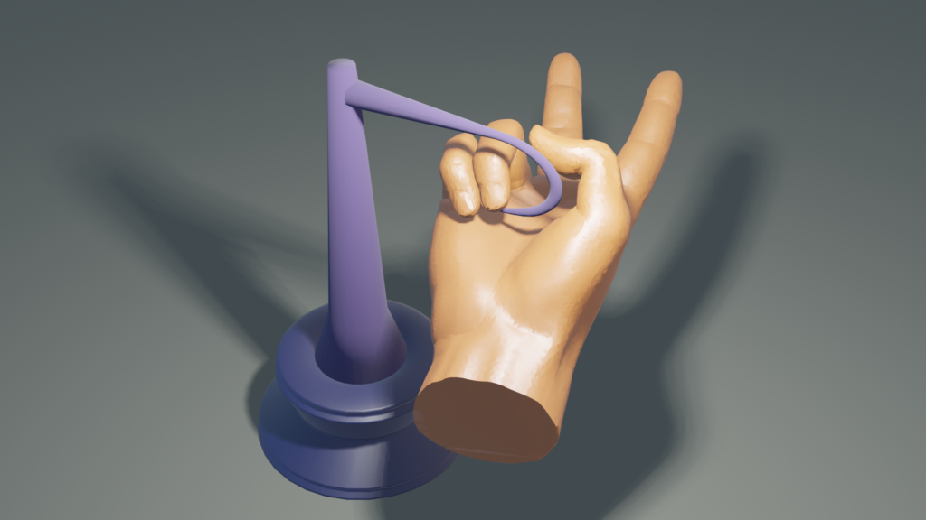
In the previous pictures, assuming constant density, each object is balanced with only one support point. Finally, we have the following hand which can be found in the Utah 3D Animation Repository.

4. Results and future work

Here we list some limitations of our project and ways in which they could be overcome.

1. Are we certain that the results obtained really fool human judgement? Our team finds these balancing objects quite surprising or, at the very least, aesthetically pleasing. We could try giving more definite proof by designing a survey. For example, people could look at different objects supported at a single point and guess if the objects would fall or not.
2. We have only verified that the objects should be stably balanced by computing the location of the center of mass. We could further test this by running physical simulations and by 3-D printing some of the examples.
3. Given a 3-D object that has already been modeled. We checked whether it could be balanced in any surprising way. One step forward would be generating 3-D models of objects that verify the properties we desire. It would be desirable that given a mesh (e.g. of an octopus), we could deform it so that the result (which hopefully still looks like an octopus) can be balanced in a surprising way.

5. Conclusion

Let’s take a step back and see this project has taught us. We started with the question: why do some objects, like the balancing bird, seem so surprising? This led us to study how people perceive objects through their center of mass and, after searching through a variety of 3D data sets, we found objects that also seem to balance in a surprising way. This was a very fun project and we really enjoyed it as a group, it involved playing with a bit of math, the geometry of triangle meshes and making beautiful visualizations while also learning something about human perception. Finally, we would like to thank Justin Solomon for organising the SGI, giving us this wonderful opportunity and Kartik Chandra for offering and mentoring such a fun project.

References

[1] Peter W Battaglia, Jessica B Hamrick, and Joshua B Tenenbaum. Simulation as an engine of physical scene understanding. Proceedings of the National Academy of Sciences, 110(45):18327–18332, 2013.

[2] Kartik Chandra, Tzu-Mao Li, Joshua Tenenbaum, and Jonathan Ragan-Kelley. Designing perceptual puzzles by differentiating probabilistic programs. In ACM SIGGRAPH 2022 Conference Proceedings, pages 1–9, 2022.

[3] Brian Mirtich. Fast and accurate computation of polyhedral mass properties. Journal of graphics tools, 1(2):31–50, 1996.

[4] Yichen Li, YingQiao Wang, Tal Boger, Kevin A Smith, Samuel J Gershman, and Tomer D Ullman. An approximate representation of objects underlies physical reasoning. Journal of Experimental Psychology: General, 2023.

Students: Francisco Unai Caja López, Shalom Abebaw Bekele and Sara Ansari
Directed by Jorg Peters and Kyle Lo

1. Introduction

The goal of this project is to design a layout simplification procedure. Following [2], we define an integer-linear programming model to find a set of collapsable arcs, and merge sets of arcs to simplify the layout. The algorithm is part of a bigger research project that is currently carried out by Kyle Lo and Jorg Peters. In said project surfaces are approximated using splines and piece-wise Bezier surfaces [7].

1.1 What is a layout and why do we care about layouts?

Definitions. Consider a graph M = (V,E) of a triangle mesh. For us, a layout is defined as another graph G = (N,A) where N is a subset of V called nodes and A is the set of arcs. Each arc a ∈ A is a polyline that connects two nodes via a sequence of edges from the original triangle mesh. For each node n ∈ N, we define its valence as the number of arcs incident to n. Also, a node is said to be a singularity if it has valence different than 4. Singularities are particularly important in quad layouts, that is, layouts in which all patches are 4-sided. This is because singularities usually lie near important regions and features of the surface. In the following figure you can see an example of a quad layout.

Another important concept in this project is that of a trace. Traces are polylines that begin at a singularity and travel through the layout until they reach another singularity. If we are building a trace and encounter a regular node n, the trace will continue through the opposite arc of n. The following figure shows 5 traces that originate at a particular singularity.

Layouts can describe the global structure of the mesh while also defining a partition. Moreover, layouts play a crucial role in tasks such as quadrangulation and embedding Bezier, or NURBS surfaces.

1.2 Layout generation and the objective of this project

There are various methods for generating quad mesh layouts, such as finding a set of separatrix candidates (i.e. paths connecting pairs of prescribed singularities) in topologically distinct ways, from which a subset is chosen to define a full layout [6]. Another method involves computing a cross-field from a given set of linear PDEs based on an imposed set of singularities. These singularities can occur naturally, for example, by minimizing Ginzburg-Landau energy, or as a user-defined singularity pattern [5]. The interested reader can learn more about layouts and quad meshes in [3].

In this project we are given layouts generated by a modified version of Quadwild [1]. These layouts are generated from triangle meshes. The goal is to find a subgraph of the layout with as few partitions as possible while ensuring that each pair of singularities is separated.

2. Finding collapsable arcs via integer programming

In order to simplify a layout, we first need to figure out which elements are removable. Precisely, we want to know when an arc can be collapsed. To do this, for each arc a ∈ A we define an integer variable q_a. We define an integer programming model following [2]. In the paper the layouts are allowed to have T-junctions which makes it so that the variables q_a can take any non negative value 0,1,2,… However, this doesn’t happen with the layouts we are working with so, just for this project, we can assume q_a is binary and defined as

\(q_a =
\begin{cases}
1 & \text{if arc } a \text{ is collapsable} \\
0 & \text{otherwise}
\end{cases}.\)

2.1. Constraints to enforce properties of the resulting layout

We have two main restrictions.

The resulting layout must be a quad layout

Suppose that we want to collapse arc a in the following figure, then we must also collapse all the arcs a’, a”, … Otherwise, we would have a three sided patch and the result would not be a quad layout.

More generally, if arcs a and a’ lie in the same patch and are opposite to each other, then we must have q_a = q_a’.

Singularities must remain separate

In general, singularities tend to appear near important features of the mesh or in regions with high curvature. Thus, it makes sense that we try to preserve their locations. We make sure that different singularities aren’t merged together regardless of the number of collapsed arcs. This is done by forcing that any pair of singularities are at a ”positive Manhattan distance”. More precisely, consider two singularities n₁, n₂ and traces t₁, t₂ with origin in n₁ and n₂ respectively. Assume that both traces go through mid node n_m, then we must have

\(\sum_{a\in t_1}q_{a} + \sum_{a\in t_2}q_{a} \geq 1.\)

In the following figure we can see an example of a pair of intersecting traces t₁ and t_2.

And in the following figure we have the set of arcs that links the origin of each trace to the mid node.

One possibility to avoid collapsing two singularities together would be, for each pair of nodes n₁, n₂, finding intersections of all possible traces t₁, t₂ and add the previous restriction to the model. In that case, the number of restrictions would be quadratic in the number of nodes. However, the same result can be achieved with far fewer restrictions as is stated in [2].

Notation. For every pair of intersecting traces t_i, t_j, we denote the first common node as n_ij. The set of arcs that link the origin on t_i with n_ij is represented by S_ij and the total length of those arcs is denoted by l_ij. Finally, given a trace t_i, we define n_i* as the intersecting node which is closest to the origin of t_i and verifies l_i* > l_*i. The set of arcs that link the origin of t_i with n_i* will be denoted S_i*.

Lemma 1 of [2] asserts that the family of restrictions

\(\sum_{a\in S_{i*}} q_a \geq 1, \quad \text{for every trace }t_i\)

implies the inequality we previously mentioned. Therefore, we can enforce the desired property using O(⎮N⎮) restrictions where ⎮N⎮ is the number of nodes.

Finally, if we just want to collapse as many arcs as possible, we could set the objective function as ∑_aq_a where the sum is over all arcs. This yields the following linear integer programming model

\(\begin{cases}
\min & \sum_{a}q_a\\
\text{s.t.} & q_a = q_{a’} \text{ whenever } a,a’ \text{ are oposites in the same patch} \\
& \sum_{a\in S_{i*}} q_a \geq 1 \quad \text{for every trace }t_i\\
& q_a\in{0,1} \quad \text{ for every arc } a
\end{cases}\)

Said model will be optimized by Gurobi, a comercial solver. The output is a set of arcs that can be collapsed while maintaining the properties we desire. In the following figure we have in red the collapsable arcs according to an optimal solution to the model

We can see that many of the original arcs are collapsable.

2.2. How do we simplify a layout?

Suppose we have chosen to collapse an arc a, then we will need to collapse a whole set of arcs in order to preserve the quad structure of the layout. This collapse will be done by merging two sets of arcs together. In the following figure we see an example with the arcs to collapse in red and the arcs to merge in purple.

In this project we have chosen to ”move one of the arcs on top of the other” although there are many other choices to do this. In the following figure you can see the simplification procedure.

3. Results and future work

In this project we have learned about layouts and developed a procedure to simplify them iteratively. In addition, solving the integer programming problem has proved to be quite fast (under 0.05 seconds for the examples tested), as the model wasn’t too big. In the following figures you can see the result of applying the simplification several times on two different layouts.

Of course, there are a lot of aspects that can be improved and directions to continue the work

1. The code we developed is far from finished. For instance, we run into problems when some of the arcs to collapse are incident to singularities. All of these special cases should be considered and dealt with appropriately.
2. Weights could be added to variables in the objective function of the integer programming model. The objective function would look like ∑_aw_aq_a. For instance, we could define

\(\qquad \qquad \qquad \qquad \qquad \qquad \qquad \bar{k}_a = \frac{\sum{r\in R}\vert k_p^r\vert }{\vert R\vert},\quad p = \underset{i=1,2}{\text{arg max }}\vert k_i^r \cdot \vec a \vert\)

where R denotes a set of vertices close to arc a and k^r_p is the principal curvature at vertex r that better aligns with the direction vector of the arc. Then, we could define

\(
\qquad \qquad \qquad \qquad \qquad \qquad \qquad w_{b}=\frac{\max_{a}\overline k_{a}-\overline k_{b}}{\max_{a}\overline k_{a}-\min_{a}\overline k_{a}}
\)

The motivation is that we want to preserve arcs that lie in sections with very high curvature. Having a really big patch in the layout that contains very different and intricate details is undesirable. For example, if we wanted to approximate them with splines, then we would need to use a very high degree. Such weighting scheme could be helpful to prevent the creation of such patches.

3. When merging two different arcs, we have chosen to place the new arc in the location of one of the arcs to be merged. Other strategies may be more successful, for instance, we could create a new arc that passes through a region of high curvature. This could help align arcs with features.

4. After the layout simplification, a smoothing procedure like [8] could be applied on all arcs to improve the quality of the results.

Finally, we would like to thank Justin Solomon for giving us such a wonderful opportunity by organizing SGI 2023 as well as Jorg Peters and Kyle for guiding us through this project.

References

[1] Pietroni, N., Nuvoli, S., Alderighi, T., Cignoni, P., & Tarini, M. (2021). Reliable feature-line driven quad-remeshing. ACM Transactions on Graphics (TOG), 40(4), 1-13.

[2] Lyon, M., Campen, M., & Kobbelt, L. (2021). Quad layouts via constrained t-mesh quantization. Computer Graphics Forum, 40(5), 305-314.

[3] Campen, M. (2017). Partitioning surfaces into quadrilateral patches: A survey. Computer Graphics Forum, 36(2), 567-588.

[4] Schertler, N., Panozzo, D., Gumhold, S., & Tarini, M. (2018). Generalized motorcycle graphs for imperfect quad-dominant meshes. ACM Transactions on Graphics (TOG), 37(6), 1-14.

[5] Jezdimirovic, J., Chemin, A., Reberol, M., Henrotte, F., & Remacle, J. F. (2021). Quad layouts with high valence singularities for flexible quad meshing. Retrieved from https://internationalmeshingroundtable.com/assets/papers/2021/08-Jezdemirovic.pdf

[6] Razafindtazaka, F. H., Reitebuch, U., & Polthier, K. (2015). Perfect matching quad layouts for manifold meshes. Computer Graphics Forum, 34(5), 219-228.

[7] Peters, J., Lo, K., & Karčiauskas, K. (2023). Algorithm 1032: Bi-cubic splines for polyhedral control nets. ACM Transactions on Mathematical Software (TOMS), 49(1), 1-12.

[8] Field, D. A. (1988). Laplacian smoothing and Delaunay triangulations. Communications in Applied Numerical Methods, 4(6), 709-712.