Advisor: Ryan Capouellez
Volunteer: Kinjal Parikh
Fellows: Erik Ekgasit, Maria Stuebner, and Anna Cole
1: Introduction
Triangles are a nice way to represent the surface of a 3D shape, but they are not smooth. The tangent vectors on a triangle mesh are not continuous.
When it comes to representing curves, we can approximate a curve using a polyline, a set of points connected with straight lines. Alternatively, we could use a spline which provides a smooth way to form a curve that passes through a set of points. Splines that represent curves are piecewise polynomial functions that trace out a curve:
\(f: \mathbb{R} \rightarrow \mathbb{R}^n\).
Similarly a 3D shape’s surface can be represented using splines that are piecewise polynomial functions:
\(g: \mathbb{R}^2 \rightarrow \mathbb{R}^3\).
The Powell-Sabin construction is a type of spline whose pieces are essentially curved triangles that can represent smooth surfaces. In this project, we aim to augment the Powell-Sabin construction to accommodate sharp features on meshes.
1.2: The Powell-Sabin Construction
A triangle mesh can be fed into an optimization algorithm that constructs a spline surface that contains (or is very close to) the points occupied by vertices of the triangle mesh. The surface is also optimized to be smooth. This is done by assigning every triangle in the original mesh a Powell-Sabin patch, the parameters of which are then chosen during optimization. Additionally, the mesh must have a UV map, which assigns each point on the mesh to a point on the plane.
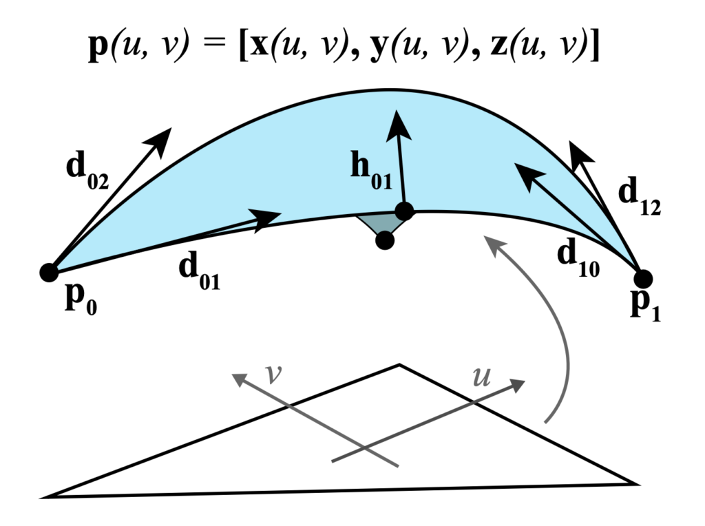
Suppose we have a triangle with indices \((i, j, k)\). Its corresponding Powell-Sabin patch can be specified using 12 vectors in \(\mathbb{R}^3\). Three position vectors \(p_i, p_j, p_k\) describe the positions of the vertices. During optimization, the vertices can move a small amount to create a smoother surface. Each vertex also gets two additional vectors to describe the derivative of the surface going out of each incident edge (labelled with \(d\) in the image below). Finally, each edge of the triangle has an associated vector to describe the derivative of the surface perpendicular to the edge at the midpoint (labelled with \(h\) in the image below).
1.3: Global Parameters
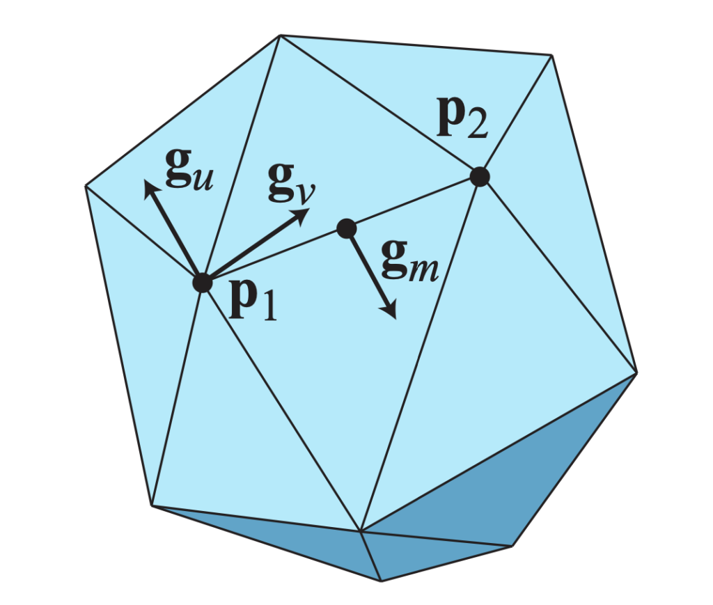
These parameters are not directly optimized. Instead they are derived from global degrees of freedom, which do get directly optimized. This allows more data to be shared between different triangles to ensure continuity. Each vertex in the mesh is assigned 3 vectors in \(\mathbb{R}^3\). One for position and two for a pair of tangent vectors, which are the gradients in the u and v directions in the local parametric domain chart. These gradients should be linearly independent unless the surface is somehow degenerate. Additionally, each edge gets one tangent vector. An illustration of these degrees of freedom is shown below.
The vectors are flattened and stored in \(q\) as follows:
\begin{equation}
q= \begin{bmatrix}
p_1 & p_2 & … & p_n & g_1^u & g_1^v & … & g_n^u & g_n^v & g_1^m & … & g_m^m
\end{bmatrix}
\end{equation}
Where \(p_i\) is the position of vertex \(i\), \(g_i^u\) and \(g_i^v\) are tangent vectors of vertex \(i\) in directions \(u\) and \(v\) (from the UV map), and \(g_j^m\) is a tangent vector for the midpoint of edge \(j\). Since the vectors are flattened, each value here ends up being three actual values in the \(q\).
Unfortunately, we lose sharp features because in \(q\) requires the tangents along an edge to be co-planar since each edge only gets 1 tangent vector. To fix this, we rip creases in half to remove the co-planarity constraint. So, we need to implement new constraints in \(q\) to ensure continuity at these cuts.
2: Experiments with Edge Ripping
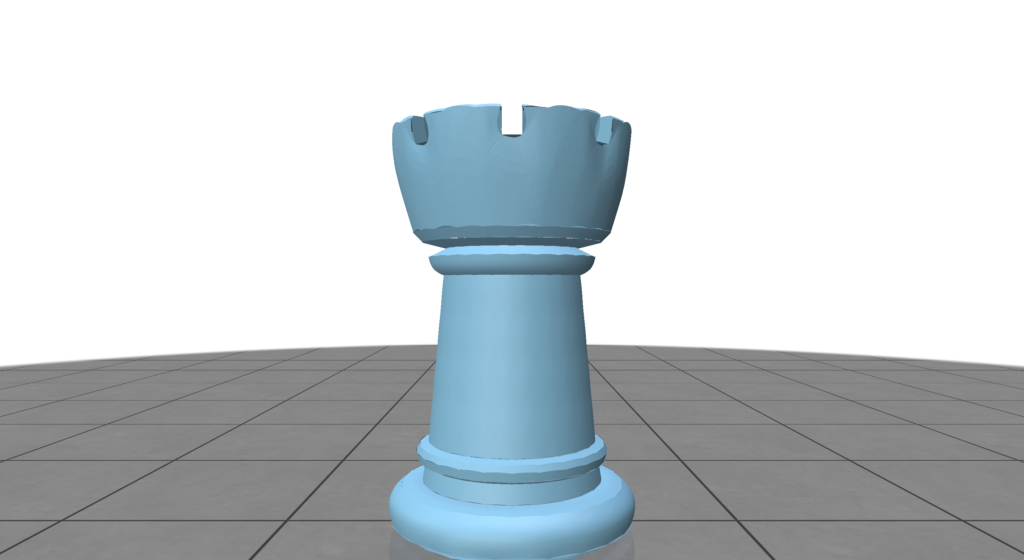
We tested ripping edges on various models. For the sake of brevity, here are the results with the chess rook model. By default the triangle mesh looks like this:
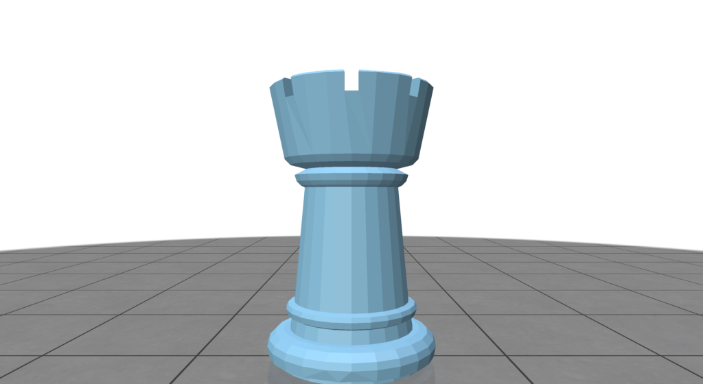
Running the base unconstrained optimization on a model of a chess rook results in a model with pretty smooth edges.
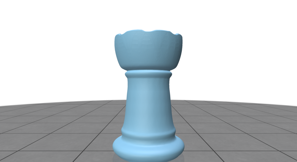
Using Blender’s Edge Split modifier, we can split each edge into two edges if the angle between their triangles (dihedral angle) exceeds 30 degrees.
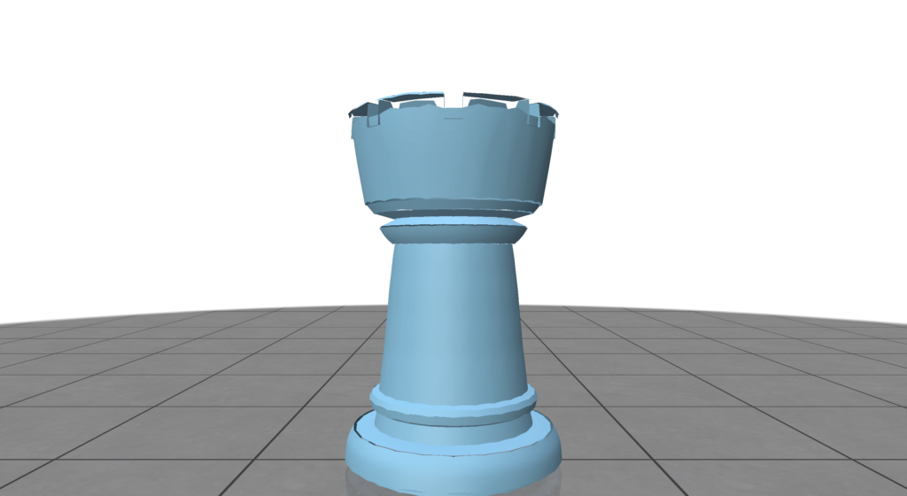
As we can see, the split edges result in gaps as the optimization process shrinks the boundaries where edges are split. There is a wave pattern at many of the edges. The pointy sections correspond to vertices and the arches correspond to edges. However, at seams where the artifacts are minimal, sharp edges definitely remain sharp.
We can force the algorithm to fit vertices near perfectly, but that still results in gaps and compromises overall smoothness.
Ripping edges results in a segmentation fault for any mesh that does not have disc topology. This is likely caused by imperfections in the UV parameterization of other shapes.
3: Quadratic Optimization with Contraints
Currently, we use unconstrained optimization. Where we find the value \(q\) that minimizes \(E(q) = \frac{1}{2}q^THq – wq^TH^fq_0 + const\). Here \(H\) is a matrix that combines fitting and smoothness energies. \(H^f\) is a matrix for just fitting energy and \(q_0\) is a vector that’s the same as \(q\) but only contains the positions of the vertices of the mesh. All other entries are 0.
Loosely speaking, \(H^f\) sums euclidean distances between vertices in the original mesh and their corresponding points on the optimized mesh. The smoothness energy is an approximation of the thin plate energy functional and discourages high curvature.
In the energy function, the first term is quadratic with respect to \(q\), the second term is linear with respect to \(q\) (since \(H^fq_0\) is a column vector that does not depend on \(q\)), and the last term is constant. Since this function is quadratic, its derivative is linear, so it’s easy to find the minimum where the derivative is equal to 0. Differentiating the function, we get \(E'(q) = Hq – wH^fq_0\). Setting this equal to 0, we get \(Hq = wqH^fq_0\) so the solution without any constraints is \(q = wH^{-1}H^fq_0\).
Suppose you have a quadratic function \(E(x) = \frac{1}{2}x^TBx – x^Tb\) and you want to minimize it subject to the constraint \(Ax = c\). If \(A\) is full row-rank (i.e. there are no redundant constraints), then the global minimizer \(x^*\) is a section of the solution to the following equation:
\(\begin{bmatrix} B & A^T \\ A & 0 \end{bmatrix} \begin{bmatrix} x^*\\ \lambda^* \end{bmatrix} = \begin{bmatrix} b \\ c \end{bmatrix}\).
4: Position Constraints
4.1: Data Organization
We want to construct and matrix \(A\) and vector \(c\) such that \(Aq = c\) is a constraint that forces duplicate vertices in \(q\) to have the same location. That is, \(Aq = c\) is true if and only if duplicate vertices share the same location. Suppose we have a pair of duplicate vertices with indices \(i, j\) where \(i \neq j\). The \(x, y, z\) coordinates of these vertices are stored in \(q\) as follows:
$$q = \begin{bmatrix}
… & p_{i, x} & p_{i, y} & p_{i, z} & …
& p_{j, x} & p_{j, y} & p_{j, z} & …
\end{bmatrix}$$
To obtain pairs of vertices that occupy the same location, we perform a naive \(O(n^2)\) sweep comparing every vertex location to every other vertex location.
4.2: Constructing Constraints
We want to constrain \(q\) such that both vertices occupy the same position. So, we want the following.
\(p_{i, x} = p_{j, x}\)
\(p_{i, y} = p_{j, y}\)
\(p_{i, z} = p_{j, z}\)
Moving all the degrees of freedom to one side, we get:
\(p_{i, x} – p_{j, x} = 0\)
\(p_{i, y} – p_{j, y} = 0\)
\(p_{i, z} – p_{j, z} = 0\)
If we’re careful with our indices, we can write the constraints as a matrix. Since each vertex in \(a\) is described with 3 entries, the indices of the \(x, y, z\) values of a vertex with index \(i\), \(p_i\) is equal to \(3i, 3i + 1, 3i + 2\) respectively. In the system \(Aq = c\), the \(k\)th entry of \(c\) will be equal to the dot product between the \(q\) and the \(k\)th row of \(A\). So, the constraint with the \(x\) coordinates can be written as \(\begin{bmatrix} 0 & … & 1 & 0 & … & -1 & 0 & …\end{bmatrix}q=0\), where 1 “lines up” with \(p_{i, x}\) and “lines up” with \(p_{j, x}\). Stacking these into a full matrix, we get something like: \(\begin{bmatrix}
… & 1 & …& & & & … & -1 & … & & \\
& … & 1 & … & & & & … & -1 & … & \\
& & … & 1 & … & & & & … & -1 & …
\end{bmatrix}q = 0\).
Where the right hand side is the zero vector. Each constraint gets it own row and each coefficient’s column in the matrix is the same as the index of its corresponding degree of freedom in \(q\).
4.3: Implementation Details
Due to restrictions with our C++ linear algebra library, Eigen, it’s actually most straightforward to insert these as entries into \(K = \begin{bmatrix}
B & A^T \\ A & 0
\end{bmatrix}\) as opposed to just \(A\). \(K\) is represented as a sparse matrix, so values can be inserted by specifying a row index, column index, and number. We can add the number of rows in $B$ to the row index to the entries in \(A\) to get the index of that corresponding point in \(K\). For values of block \(A^T\) we can just swap the row and column indices of values of block \(A\).
Proof:
Suppose you have a matrix \(K = \begin{bmatrix}
B & A^T \\ A & 0
\end{bmatrix}\) where \(B\) is square. Then, \(K_{i,j} = K_{j,i}\) if \(i, j\) index a point in block A. By the properites of block matrices, \(K^T = \begin{bmatrix}
B^T & A^T \\ (A^T)^T & 0
\end{bmatrix} = \begin{bmatrix}
B^T & A^T \\ A & 0
\end{bmatrix}\) For all entries that are not in block \(B\), \(K = K^T\), so swapping the row and column indices results in the same value. Since entries in block \(A\) are not in block \(B\), \(K_{i,j} = K_{j,i}\) for all \(i, j\) in block \(A\).
Next Steps
As of time of writing, this project is not yet complete. Several pieces of code must be combined to get position constraints working. After that, we must formulate and implement constraints on vertex tangents.