Tag: voronoi lattices

Fellows: Sanjana Adapala, Sara Ansari, Shalom Abebaw Bekele, Kyle Onghai
Volunteers: Gemmechu Hassena, Kinjal Parikh
Mentor: Andrew Spielberg

Introduction

What does the title mean in simple words?

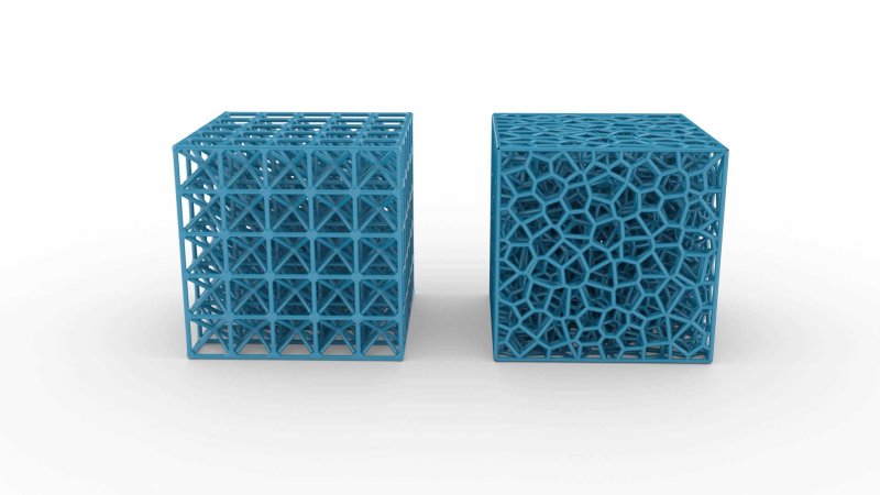
To explain the somewhat amorphous, ambiguous title of our project, let us break down the title one piece at a time.  First, what are “lattice structures”?  The simplest way to describe a lattice structure is a repeated pattern that fills a region, e.g. an area in two-dimensional space or a volume in three-dimensional space.  There are three variants of lattices: periodic, aperiodic, and stochastic.  The giveaway for whether a lattice is periodic is if the repeated pattern looks like it’s formed by “copying” a portion of the lattice and “pasting” it throughout the entire region; think of a sheet of graph paper.  Aperiodic lattices are those that are, well, not periodic.  If you can’t find some repetition in the structure, chances are it is aperiodic.  Stochastic lattices are characterized by their probabilistic manufacturing.  One of the most well known stochastic lattices, and the one which we have focused our attention on, is the Voronoi lattice.

What is a Voronoi Lattice?

A Voronoi lattice is a space/volume partitioned into regions near each of a given set of points. The regions are known as Voronoi cells, and they are defined as the set of all points in the plane that are closer to one point than any other. A Voronoi lattice can be generated in three dimensions by placing a set of points on a plane and then drawing a bisecting line equidistant between each point to its nearest neighbor.

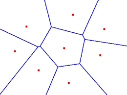
From the above image we can see that the lines are drawn in such a way that they are equidistant to each and every point with its neighbor.

Why do we care about Voronoi Lattices (mechanically)?

Voronoi lattices are of interest in mechanics and metamaterials because they exhibit a wide range of mechanical properties depending on cell shape and arrangement. Voronoi lattices can be made very stiff, very light, or have a negative Poisson’s ratio. Voronoi lattices are used in mechanics to simulate the mechanical behavior of porous materials, the shape and arrangement of cells can also be used to predict the material’s stiffness, strength, and fracture toughness. Voronoi lattices can also be used in metamaterials to create materials with unusual optical and electromagnetic properties. Voronoi lattices can be used to create negative refractive index metamaterials that can be used to bend light around corners.

What are the design parameters of Voronoi Lattices?

We take inspiration for the design parameters from the work of Martínez et al., who considered two design parameters in their procedural algorithm to manufacture open-cell Voronoi foams: the density of the seeds/nuclei and the thickness of the beams.  By modifying both these parameters on the fly, they were able to finely control the elasticity in their prints.

Why is resilience in Voronoi Lattices interesting (applications?)

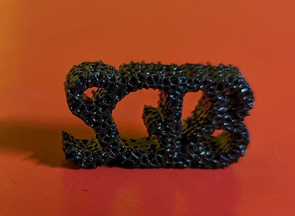
Resilience in Voronoi lattices is interesting as it can improve the mechanical properties of a material in such a way that it allows the material to withstand damage when subjected to shock and/or vibration.  In addition, during the curing of a 3D printed Voronoi foam, clogging within the vertices and beams of a Voronoi foam often occurs randomly.  A better understanding of resilience will tell us what properties we can expect our Voronoi lattice to keep when some beams are clogged.

What do we want to prove or demonstrate about the probabilistic nature of these lattices, and why?

Our goal would be to have a model that could accurately predict how many beams and/or vertices would fail, where beam or edge failure may occur, and the probability that certain properties, e.g. connectedness, of the lattice will remain intact given that there may be some clogged vertices or edges.  These details could help us fine tune the microstructure of our prints so that we can reduce the chance of clogging enough to ensure the foam will have certain properties we desire with high probability.  This will make printing more efficient than the current trial-and-error method.

Random Graphs and Voronoi Lattices

A random graph is obtained by starting with a set of n isolated vertices and adding successive edges between them at random. Random graph models produce different probability distributions on graphs. Some notable models include:

• \(G(n, p)\) – proposed by Edgar Gilbert: Every possible edge occurs independently with probability 0 < p < 1. The probability of obtaining any one particular random graph with m edges is  \(p^m(1-p)^{{n \choose 2}-m}\)
• \(G(n,m)\) – Erdős-Rényi model:  Assigns equal probability to all graphs with exactly \(m\) edges, i.e.,  \(0 ≤ m≤ n\), each element in \(G(n,m)\) occurs with probability \({{n \choose 2} \choose m}-1\)

The connection between Voronoi lattices and random graphs arises when studying spatial processes that involve both distance-based interactions and randomness. Some examples include:

1. Voronoi Percolation Model: In this model, a Voronoi lattice is used as a framework to represent the spatial distribution of points, and edges are randomly added between points based on some probability. This can result in a network of interconnected Voronoi cells, with the properties of the network dependent on the probabilities of edge connections.
2. Random Voronoi Tessellations: Instead of using a fixed set of seed points, you can consider generating a random set of seed points and constructing a Voronoi tessellation based on these random points. The resulting Voronoi cells may exhibit interesting statistical properties related to random processes.
3. Spatial Random Graphs: These are random graph models where nodes are distributed in a space, and edges are added based on a certain spatial rule and a random component. In some cases, the edges might be determined by proximity (similar to Voronoi regions) and a random chance of connection.

Our goal here is to study the probability of properties such as connectedness, with constant probability that a lattice beam will fail. The equivalent graph theory problem would be: what happens to properties of a random graph, such as connectedness when the probability of deleting an edge is constant.

Suppose we delete the edges of some graph \(H\) on vertex set \([n]\) from \(G_{n,p}\). Suppose that \(p\) is above the threshold for \(G_{n,p}\) to have the property. We discuss the resilience of the property of connectedness. For our first approach, we explore the concept of Hamiltonian cycles and r regular random graphs. In the book, we define the concept of pseudo randomness. If a subgraph of a graph is pseudorandom, we conclude that a graph has a Hamiltonian cycle. How does the existence of the Hamiltonian cycle relate to connectivity? Having a Hamiltonian cycle is stronger than the property of connectedness. So, if we are able to find a pseudo random sub-graph for a graph H, we will be able to conclude the property of connectedness for that cycle.

The second approach is as follows: we relate this property to a Voronoi lattice. We can refine the \(G_{n,m}\) graph so that the vertices have a fixed equal degree sequence d. This is called a uniformly distributed \(r\)-regular graph. We can see that clearly a Voronoi lattice can be modeled as a \(r\)-regular graph. We can show with high probability that random \(d\)-regular graphs are connected for \(3\leq d\). Further, for large graphs, we can show that \(G_{n,m}\) can be embedded in a random r-regular graph. So, the graph obtained by removing edges can be modeled as a \(G_{n,m}\), which by the above property can be embedded into a Voronoi lattice.

The above listed ideas are certainly not an exhaustive of the several other approaches to theoretically approaching this problem. The next section explores an extension of this idea, where the probability of failure is variable.

Distribution of Edge Lengths

What if the probability of a beam clogging is proportional to beam length?  Intuitively, a long beam ought to be more prone to clogging than a short one since there are more places where a clog can form.  A model accounting for this would have the probability of a beam of length \(I\) failing is proportional to \(I/L\) where \(L\) is the length of the longest beam in the foam.  In order to analyze this model, we must first describe the distribution of edge lengths of the foam.   So, motivated by this problem, we set out to determine the distribution of edge lengths of a random spatial (i.e. three-dimensional) Voronoi tessellation.  To be precise, the random point process used to generate the Voronoi tessellation that we consider here, is a homogeneous Poisson point process.  A Poisson point process is a method of randomly generating points in a space where the number of points follows a Poisson distribution.  The point process is homogeneous if the distribution of the points themselves is uniform. Martínez et al. generate their Voronoi foams by a slight variation of the homogeneous Poisson point process in their paper, so the results we list below should be decently accurate. 

Fortunately, several geometric characteristics of this so-called Poisson-Voronoi tessellation have been studied for decades now, both analytically and through simulation.  In the spatial case, Meijering showed that the mean edge length is

$$E(L) = \frac{7}{9} \left( \frac{3}{4 \pi} \right)^{\frac{1}{3}} \Gamma \left( \frac{4}{3} \right) \rho^{-1/3}$$

where \(\rho\) is the intensity of the underlying Poisson point process.  Since then, Brakke determined an integral formula for all the higher moments of the edge length when \(\rho = 1\).

$$E \left( L^n \right) = \frac{35}{36} \pi^{-n/3} \Gamma \left( 4+\frac{n}{3} \right) \int_{-\pi/2}^{\pi/2} \int_{-\beta_1}^{\pi/2} B^{-4-n/3} \left( \tan \beta_1 + \tan \beta_2 \right)^n \sec^2 \beta_1 \left( \sec \beta_1 + \tan \beta_1 \right)^2 \sec^2 \beta_2 \left( \sec \beta_2 + \tan \beta_2 \right)^2 d\beta_1 d\beta_2$$

Here, if \(S_0\), \(S_1\), and \(S_2\) are three common seeds of an edge and \(Q\) is their circumcenter, then \(\beta_1\) is the angle \(QS_0S_1\), \(\beta_2\) is the angle \(QS_0S_2\), oriented so that \(\Phi_2 = \beta_2-\beta_1\) where \(\phi_2\) is the azimuthal angle of \(S_2\) is a system whose north polar axis contains \(S_1\) .  The quantity \(B\) is defined by 

$$B = \sec^3 \beta_1 \left( \frac{2}{3} + \sin \beta_1 – \frac{\sin^3 \beta_1}{3} \right) + \sec^3 \beta_2 \left( \frac{2}{3} + \sin \beta_2 – \frac{\sin_3 \beta_2}{3} \right).$$

Moreover, Brakke described the probability density function when $late \rho = 1$.  The distribution of edge lengths \(L\) is

$$f_L(L) = 12 \pi^6 L^{11} \int_{-\pi/2}^{\pi/2} \int_{-\beta_1}^{\pi/2} e^{-\pi L^3 B \left( \tan \beta_1 + \tan \beta_2 \right)^{-3}} \left( \tan \beta_1 + \tan \beta_2 \right)^{-12} \sec^2 \beta_1 \left( \sec \beta_1 + \tan \beta_1 \right)^2 \sec^2 \beta_2 \left( \sec \beta_2 + \tan \beta_2 \right)^2 d\beta_1 d\beta_2.$$

Many of these results have been generalized to higher dimensions and arbitrary intensities, c.f. Calka for further references.  This information should sufficiently characterize the distribution of edge lengths for us to set the proportionality constant appropriately and estimate the length of the longest beam in the foam, making the development of this model more feasible.

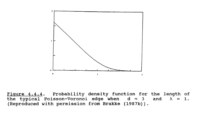
Without the proper background, it is hard to justify these formulas.  Rather than delve into the proofs, we felt it would be more practical and interactive to simulate the spatial Poisson-Voronoi tessellation and compute the edge lengths in C++ using Rycroft’s Voro++ library.  If you’d like to run the code yourself, please do so!  We have published the code on GitHub.  After running the simulation on 50 different Voronoi diagrams, we obtained a mean edge length of 0.430535 and variance of 0.113877, which aligns quite decently with the values Brakke computed.

It is worth noting that the geometric analyses presented above study infinite tessellations, and our simulation assumes periodic boundary conditions in order to remain consistent with this fact.  However, we would ideally like statistics in the case where there is a boundary; these would be more relevant to procedural Voronoi foams since our prints obviously are not infinite.  Additionally, the microstructure is intentionally aperiodic so that we can grade the elasticity of our prints and constrain the lattice structure to the boundary of the print, so using periodic boundary conditions is less than ideal.  Still, our analysis should be applicable to regions away from the boundary as long as we vary the intensity appropriately.  We would like to explore the  exact differences in the finite case further.

Speaking of directions to continue this work in, the details of how to apply this knowledge to model the resilience of a Voronoi foam as a model remain a mystery.  We may be able to relate the two through soft random geometric graphs, so we hope to pursue this potential direction in the future.

Voronoi Tessellations Used to Simulate Pre- and Post-mechanical Behavior of Concrete Beams

Voronoi tessellations can be used in conjunction with a kinematic mesoscale mechanical model to reliably simulate the pre- and post-critical mechanical behavior of concrete beams. These high-fidelity models depict concrete as a collection of rigid bodies linked together by cohesive contacts. Concretes have discrete jumps in the displacement field due to their rigid bodies, and the detailed representation of a complex, interconnected, and highly anisotropic crack structure in the material makes the discrete models ideal for use in the coupled multiphysical analysis of mechanics and mass transport.

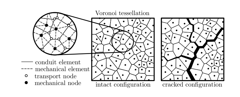
The left-hand side represents  a tessellation of a 2D domain into (i) ideally rigid Voronoi cells for the mechanical problem and (ii) Delaunay simplices representing control volumes for the mass transport problem. The right-hand side represents deformed state with opened cracks creating channels for mass transport.

In a discrete framework, it is preferable to replace locally cheap, low-fidelity models with detailed, expensive high-fidelity models in areas where they are required. The finite element approximation of a homogeneous continuum is typically low-fidelty. 

A heterogeneous material is represented by an interconnected system of ideally rigid particles. These polyhedral particles are thought to represent larger mineral grains in both concrete and the surrounding matrix. The Voronoi tessellation, which is built on a set of randomly distributed generator points within a volume domain, generates particle geometry. The generator points are added to the domain sequentially with a given minimum distance lmin, which determines the size of the material heterogeneities.

As a result, it is convenient to use a fine discritization/high fidelity model in areas where it is required because it helps to maintain the quality of results while keeping the computational cost at a reasonable level.

The geometrical representations of mechanical and conduit elements are linked by the Voronoi-Delaunay structure duality. To achieve simultaneous refinement in both structures, it is sufficient to refine the Voronoi generator points. Because cracking is the only source of non-linearity in the mass transport part, the adaptive refinement is governed solely by the mechanical part of the model.

When a selected criterion in any rigid particle exceeds a given threshold, these high fidelity models are activated. Then, a particle’s neighborhood is refined.

The refinement procedure is now detailed. Initially, the domain is discretized into relatively coarse particles with sizes determined by strain field gradients (excessively large particles may not accurately approximate the elastic stress and pressure state). lmin,c is the minimum distance between Voronoi generator points in the coarse structure. Because cracking coupling and inelastic mechanical behavior are both dependent on the size of rigid particles, such a model can only be used in the linear regime.

The average solid stress tensor for each particle is computed at time \(t+t\) after each step of the iterative solver (in the state of balanced linear and angular momentum and fluid flux). The refinement criteria are evaluated in all particles except those belonging to the refined physical discretization – in our case, the Rankine effective stress is compared to 0.7 multiple of the tensile strength. Critical particles are detected as they approach the inelastic regime.If no such critical particles exceed the threshold stress, the simulation proceeds to the next time step. If the entire time step is rejected, the simulation time is reset to t. Internal history variables at time \(t\) are also saved, including the damage parameter, \(d\), and maximum strains, \(\max eN\) and \(\max eT\), of the contacts in the refined part of the model. 

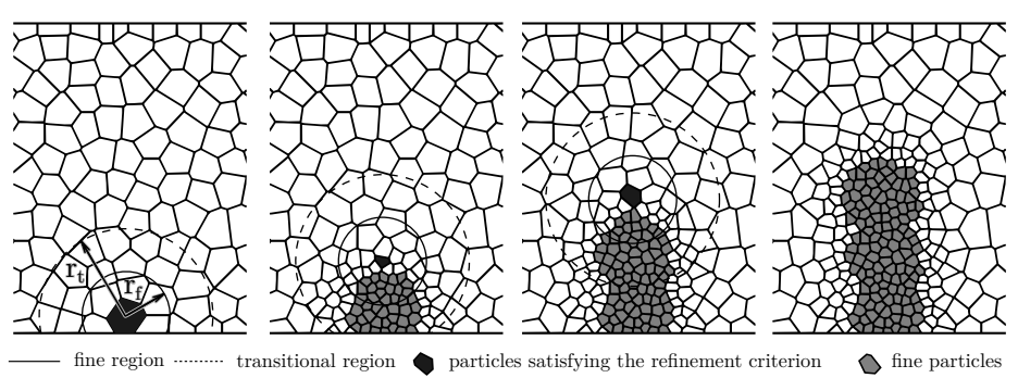
Following that, the Voronoi generator points that define the model geometry are updated, and regional remeshing to fine physical discretization is performed. In the physical discretization, the minimum distance between Voronoi generator points is denoted as lmin,f. All generator points that do not belong to the fine physical discretization are removed within the spheres of radii ‘rt’ around the centroids of each critical particle, as shown in. Those from physical discretization are retained. New generator points are then inserted into the cleared regions with (i) the minimum distance corresponding to the physical discretization, \(\mathrm{lmin,f}\), in the spheres of radii \(rf\), and (ii) the minimum distance increasing linearly from \(\mathrm{lmin,f}\) to \(\mathrm{lmin,c}\) as the distance from the critical particle changes from \(rt\) to \(rf\). Model parameters \(rf\) and \(rt\) are these two radii. The updated set of generator points is then used to generate the model geometry again.

Finally, Voronoi tessellations in conjunction with a kinematic mesoscale mechanical model provide a reliable method for simulating the mechanical behavior of concrete beams. These high-fidelity models accurately capture the discrete jumps in the displacement field and the intricate crack structure of concrete by representing it as a collection of rigid bodies linked together by cohesive contacts. This makes them ideal for investigating coupled multiphysical mechanics and mass transport in concrete. When working with a heterogeneous material such as concrete, it is advantageous to replace locally low-fidelity models with detailed, expensive high-fidelity models in areas where they are required. The Voronoi tessellation is a convenient way to generate particle geometry while also refining the mechanical and conduit elements. The model achieves a higher level of accuracy without significantly increasing the computational cost by refining the Voronoi generator points. For those interested in learning more about Voronoi tessellations and their applications in concrete modeling, we recommend reading more about them. Understanding and implementing these techniques can significantly improve simulation accuracy and reliability, allowing for more precise analysis of concrete behavior and the development of more effective engineering solutions.

Random Graphs

What is a Random Graph? 

The study of Random graphs was initiated  by Erdos and Renyi. There are two related ways of generating a random graph that Eros and Renyi came up with:

1. Uniform Random Graph (\(G_{n,m}\)): \(G_{n,m}\) is the graph chosen uniformly at random from all graphs with m edges. Let \(\mathscr{G}_{n,m}\) be the family of all labeled graphs with n nodes and m edges, where 0 ≤ m ≤ (n 2). To every graph \(G\in \mathscr{G}_{n,m}\), assign a probability \(P(G) = {{n\choose 2} \choose m}^{-1}\). Or, equivalently, start with \(n\) nodes and insert \(m\) edges in such a way that all possible \({n \choose 2}\)  choices are equally likely.

2. Binomial Random Graph (\(G_{n,p}\)): For \(0 ≤ m ≤ {n \choose 2}\), assign to each graph \(G\) with \(n\) nodes and \(m\) edges a probability \(P(G) = p^m (1-p)^{{n \choose 2}-m}\) where \(0 ≤ p ≤ 1\). Or equivalently, we start with an empty graph with n nodes and do \({n \choose 2}\) Bernoulli experiments inserting edges independently with probability p.

They are related by the lemma that given a binomial random graph and it is known that it has m edges, then the graph is equally likely to be one of the \({{n \choose 2} \choose m}\) graphs that has \(m\) edges. Thus \(G_{n,p}\) conditioned on the event \(\{G_{n,p} \text{ has m edges}\}\) is equal in distribution to \(G_{n,m}\). We refine the model \(G_(n,m)\) so that, if we pick a graph from the set of graphs with \(n\) nodes and \(m\) edges, it has a fixed degree sequence \((d_i,..,d_n)\). Recall a degree sequence is the degrees of each vertex in the graph listed in non-increasing order. In the case when the degrees are the same i.e. \(d_i = .. = d_n\), the graph is called a uniformly random r-regular graph.

Now, we are interested in generating a random graph from a given degree sequence and a method for doing so was proposed by Bollobas called the Configuration Model. The configuration model is useful in estimating the number of graphs with a given degree sequence, and for our purposes showing that, with high probability, random \(d\)-regular graphs are connected for \(3\leq d = O(1)\).

The Configuration Model

To given an overview of how the configuration model works, it assigns to each node \(i\) a total of \(W_i\) “half-edges” or “cells” where \(|W_i| = d_i\). There are \(\Sigma_i W_i = 2m\) half-edges, where \(m\) is the number of edges of the graph. Then, two half-edges are chosen uniformly at random and connected together to form an edge. Then, another pair of edges is chosen uniformly at random from the remaining \(2m-2\) half-edges and connected, this process is repeated until all the half-edge pairs are exhausted. The resulting graph has the degree sequence \((d_i,..,d_n)\).

Let’s take a deeper look into the configuration model. This section uses the explanation offered by __ in ___. Let the degree sequence \(D = (d_1, d_2, …, d_n)\) where \(d_1 + d_2 + … + d_n = 2m\) is even and \(d_1, d_2, …., d_n \geq 1\) and \(\sum_{i=1 to n} d_i(d_i-1) = \Omega(n)\). Let \(\mathscr{G}_{n,d} = \{ \text{simple graphs with } n \text{ such that } \mathrm{degree}(I) = d_i, i \in {1,..,n}\}\). Randomly pick a graph \(G_{n,d}\) from \(\mathscr{G}_{n,d}\).

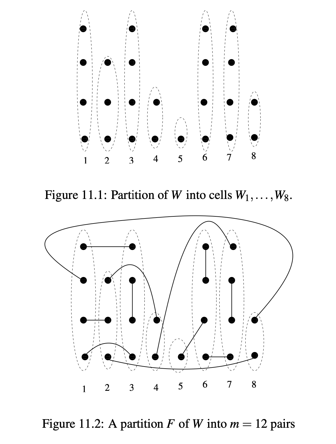
Now, let us generate the random graph \(G_{n,d}\) given a degree sequence that satisfies the above constraints. Let \(W_1, W_2, …., W_n\) be a partition of a set of points \(W\) where \(|W_i| = d_i\) for \(1 \leq i \leq n\). We will assume some total order \(<\) on \(W\) and that \(x < y\) if \(x\in W_i, y\in W_j\) where \(i< j\). For \(x\in W\) define \(\varphi(x)\) by \(x\in W_{\varphi}(x)\). We now partition \(W\) into \(m\) pairs, call this partition (or configuration) \(F\). We define the (multi)graph \(\gamma(F)\) as \(\gamma(F) = ([n],\{(\varphi(x), \varphi(y)) : (x,y)\in F\})\). 

Denote by \(\Omega\) the set of all configurations defined above for \(d_1 + · · · + d_n = 2m\) 

Let’s look at an example:

Here \(n = 8\) and \(d_1 = 4,d_2 = 3,d_3 = 4,d_4 = 2,d_5 = 1,d_6 = 4,d_7 = 4,d_8 = 2\).

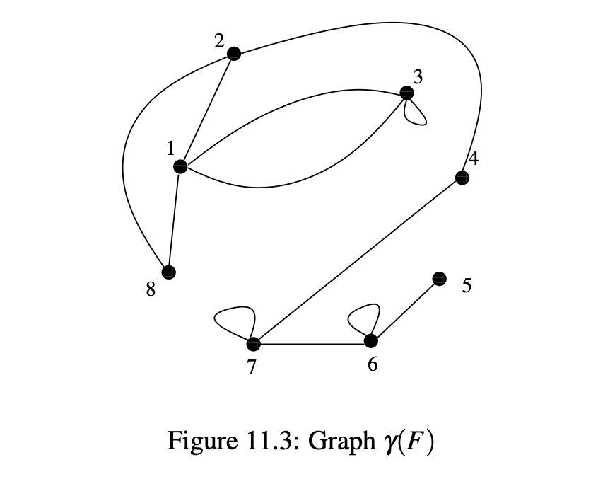
The following lemma gives a relationship between a simple graph \(G\in \mathscr{G}_{n,d}\) and the number of configurations \(F\) for which \(\gamma(F) = G\).

Lemma 11.1. If \(G\in \mathscr{G}_{n,d}\), then \(n |\gamma^−1(G)| = \prod d_i!\).  

That is, we can use random configurations to “approximate” random graphs with a given degree sequence. A useful corollary allows us to pick \(\gamma(F)\) for a random choice of \(F\) if and only if \(\gamma(F)\) is a simple graph (has no loops or multiple edges) as opposed to sampling from the family \(\mathscr{G}_{n,d}\) and only accepting graphs that satisfy certain properties.

We are interested in connectivity of random graphs, and thus Bollobas’ use of the configuration model to prove the following connectivity result for an \(r\)-regular graph: 

Theorem 11.9. \(G_{n,r}\) is \(r\)-connected with high probability. Here, \(G_{n,r}\) denotes a random \(r\)-regular graph with vertex set \([n]\) and \(r ≥ 3\) constant.  

Conclusion

Let us conclude by discussing the synergies of the four directions we researched.  Our study of random graphs and the distribution of edge lengths both aimed to make headway on the problem of modeling beam failure in Voronoi foams.  The former work is applicable when the probability of beam failure is constant whereas the latter offers some results that would be necessary if the probability is proportional to edge length.  Although we initially thought modeling the simpler constant-probability case might provide some insight into how to model the proportional-to-edge-length case, the theorems regarding random graphs that we used to model the constant-probability case are contingent on a fixed probability.  Instead, we think that studying soft random geometric graphs may offer more insight in the proportional-to-edge-length case.

Additionally, Voronoi tessellations can be used to create discrete representations of materials, and allows one to study the mechanical behavior and properties of a material to further analyze the complex mechanical behaviors.

References

Brakke, Kenneth A.. “Statistics of Three Dimensional Random Voronoi Tessellations.” (2005).

Calka, Pierre. New Perspectives in Stochastic Geometry. Edited by Wilfrid S. Kendall and Ilya Molchanov, Oxford University Press, 2010.

Martínez, Jonàs et al. “Procedural voronoi foams for additive manufacturing.” ACM Transactions on Graphics (TOG) 35 (2016): 1 – 12.

Møller, Jesper. Lectures on Random Voronoi Tessellations. Springer, 1994. DOI.org (Crossref), https://doi.org/10.1007/978-1-4612-2652-9.