Fellows: Yufan Hu, Robiul Islam Hannan, Kabir Sahni
Mentor: Yusuf Sahillioglu
Volunteer: Vivien van Veldhuizen
Introduction:
Developable surfaces are surfaces that can be unfolded onto a plane without stretching, compression, or other geometric distortion. They are relevant to applications in geometric design, digital fabrication, manufacturing, architecture, and related areas where three-dimensional geometry must be represented or fabricated from planar material. In continuous setting developable surface is charecterized by Gaussian curvature. The Gaussian curvature is formulated as:
- means surface is locally a bowl-like shape
- means surface is locally flat in at least one direction
- means surface is locally a saddle-like shape
Our objective was to minimize non-flat curvature regions while preserving the geometric characteristics of the original surface. To address this problem, we formulated three vertex-based optimization techniques- normal one-ring, double-cone, and virtual-sphere– to relocate vertices through constrained directional searches while minimizing local angle-defect curvature. A complementary 3D-grid-based local search method explores possible vertex movements in the local normal and tangent directions. It then selects the movement that reduces the curvature while maintaining the surface geometry and preventing changes in triangle orientation.
Algorithm 1: Vertex relocation methods
Overview
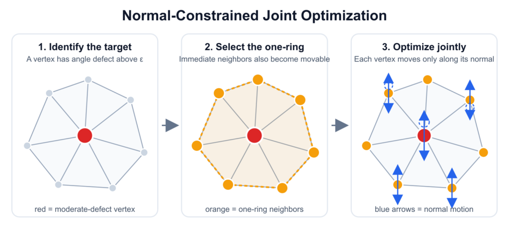
All three methods restrict vertex motion to one-dimensional directions. However, only the double-cone and virtual-sphere methods explicitly sample and search along multiple rays, while the normal-constrained method jointly optimizes scalar displacements along vertex normals.
Normal joint optimizer
We use the angle defect to measure discrete Gaussian curvature at each interior vertex. A vertex is considered approximately developable when its absolute angle defect is below a prescribed threshold:
- Vertices satisfying are classified as moderate-defect vertices and selected as optimization targets.
- Vertices whose initial angle defects satisfy are treated as singular vertices and remain fixed, since the unavoidable curvature of the surface should be preserved somewhere.
Moving one vertex changes the corner angles and angle defects of its neighbors. Therefore, we jointly optimize each moderate-defect vertex together with its one-ring neighborhood. During one optimization step, each movable vertex is restricted to move along its current normal
Here, is the fixed vertex normal during the current optimization step, and is the scalar displacement being optimized. This converts the vertex relocation problem from three variables per vertex to one variable per vertex, while still allowing neighboring vertices to move together.
The main objective penalizes only the part of the angle defect that exceeds the threshold:
The monitored set contains the movable vertices and their neighbors. A vertex contributes zero energy once it satisfies . Evaluating the energy over the neighborhood is important because reducing curvature at one vertex may transfer curvature to nearby vertices.
The complete objective combines this curvature term with regularization terms:
The remaining energy terms control how the mesh is deformed:
- weakly encourages smaller angle defects
- preserves curvature around singular vertices
- limits vertex displacement
- encourages neighboring vertices to move smoothly, and
- penalizes relative edge-length changes.
Together, these terms prevent the optimizer from reducing angle defect by introducing excessive displacement, irregular local motion, or severe geometric distortion.
Double-cone optimizer
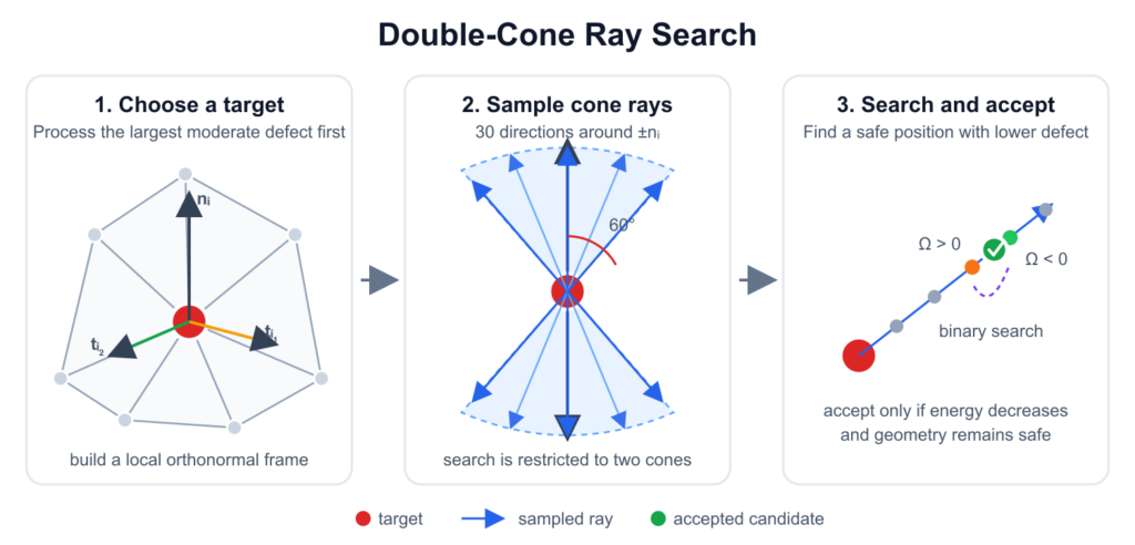
The double-cone optimizer processes moderate-defect vertices sequentially, starting with the vertex having the largest absolute angle defect. At each target vertex, it samples movement directions from two cones centered on the positive and negative vertex-normal directions.
Using the local orthonormal frame (), an outward ray is defined as
We sample 30 rays using a cone half-angle of (). The golden-angle sequence distributes the rays around the vertex normal.
Along each ray, candidate positions are parameterized by
The search distance limits both the current movement and the total displacement from the original mesh. We first evaluate five coarse intervals along each ray. If two consecutive samples contain a sign change in the angle defect, binary search is used to locate a near-zero-defect position.
A candidate is accepted only if it reduces the curvature objective and passes the geometric safety checks, including triangle orientation, area preservation, edge distortion, and cumulative displacement limits.
The cone construction is used only to generate search directions; the method does not compute the Shape Diameter Function.
Virtual-sphere optimizer
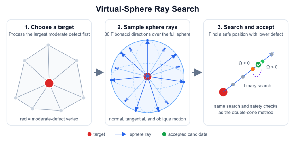
The virtual-sphere optimizer uses the same search procedure, binary search, objective function, sequential updates, and geometric safety checks as the double-cone method. The only difference is how the ray directions are generated.
Instead of restricting the directions to two cones around the vertex normal, we use a Fibonacci sphere to distribute (m) rays over the entire unit sphere:
This allows the vertex to move in unrestricted normal, tangential, and oblique directions. Our current experiment uses (m=30) rays.
Algorithm 2: Grid-based method
Overview
This method proposes a local derivative-free optimization approach for reducing the non-flat curvatures of the triangle mesh while preserving the shape. We first describe the mathematical background of the algorithm and later explain how it reduces non-flat curvatures.
3D-grid local search with orientation protection
Step1:Gaussian curvature approximation
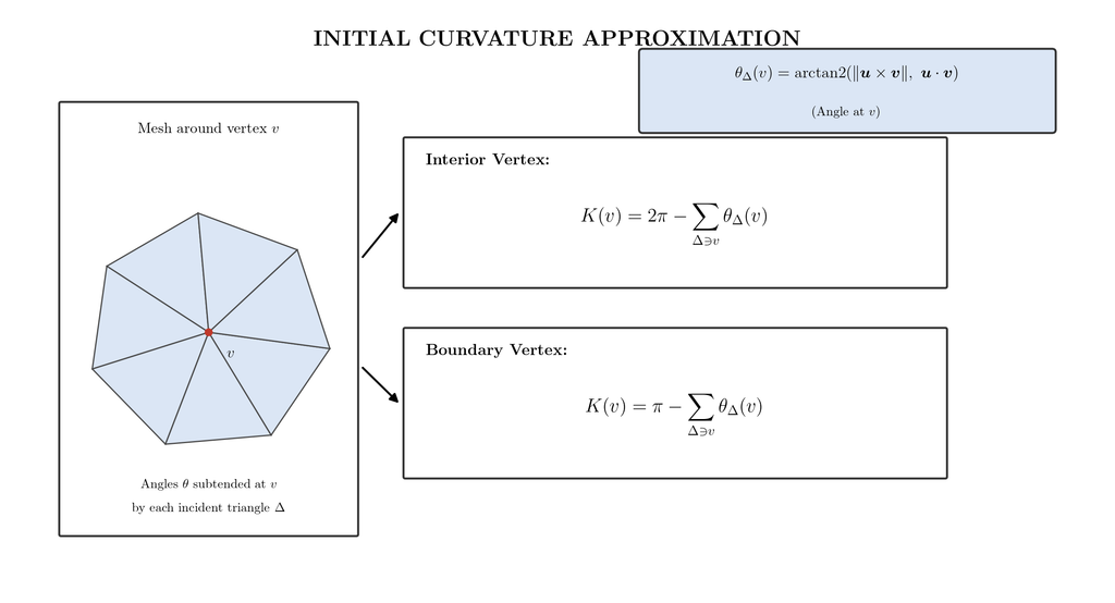
The algorithm uses the Gauss-Bonnet standard discretization formula for triangulated surfaces to estimate discrete Gaussian curvature at each vertex.
Here, and denote the sets of interior and boundary vertices. represents the interior angle of triangle Δ at vertex . is calculated using the following formula:
is the cross product proportional to the and is proportional to the .
Step2:
Local Coordinate Frame Construction:
To parameterize the local search space around a vertex, the algorithm constructs a customized local coordinate frame using the vertex unit normal vector and two orthogonal tangent vectors . is an arbitrary reference axis not parallel to
3D Grid Vector:
We introduce a 3D sampling grid using the equation by choosing a linear combination of the basis vectors. Here, the step offsets are sampled from a uniform range bounded by a maximum displacement step . Crucially, the normal displacement is scaled down by a damping factor which helps preserve mesh structure and fine geometric details.
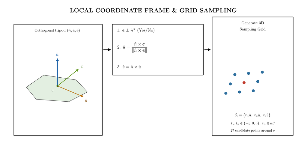
Step4: Triangle normal calculation and orientation protection
The algorithm enforces a strict face-inversion constraint of all triangles incident to the moving vertex to ensure that the vertex displacement does not compromise the topological integrity. For any candidate vertex position, the updated unit normal vector is calculated via. The algorithm then evaluates the dot product between this candidate normal and the face’s original, unmodified normal
. By requiring , the algorithm imposes a lower strict bound that rejects any vertex update causing an adjacent triangle distortion. This function prevents mesh flipping, severe distortion, and self-intersection during local search.
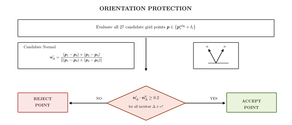
Step5:
Energy objective function:
minimizes the local Gaussian curvature defect at vertex to smooth irregularities. evaluates Gaussian curvature changes on all 1-ring neighbour vertices . this indicator term applies a penalty if a move creates curvature spikes above threshold . The regularization term penalizes to prevent excessive surface drift.
Optimization:
The optimization evaluates candidate positions from the discrete 3D sampling grid set {} alongside the original position . It greedily selects the candidate position that minimizes the energy objective , ensuring the orientation protection constraint.
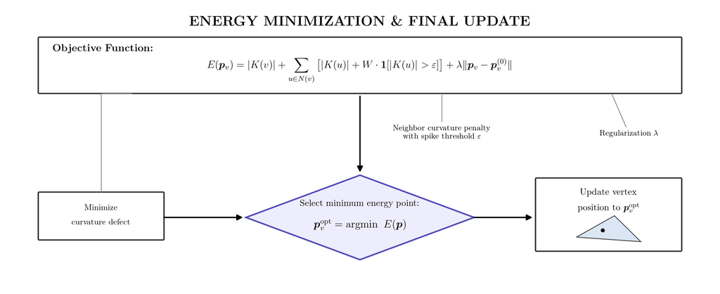
Curvature Reduction and Geometry Preservation
We compare the four operators from two perspectives: curvature reduction and geometry preservation. Curvature-related metrics evaluate how effectively each operator reduces non-flat regions, while geometry-related metrics measure the corresponding deformation and mesh-quality loss.
Table 1: Curvature-state changes.
The transition counts are selected to distinguish corrected curvature violations from newly introduced ones. The final moderate-gray count measures the remaining non-flat vertices, while threshold energy describes the severity of these violations..
| Family | Operator | Gray → Yellow ↑ | Yellow → Gray ↓ | Net reduction ↑ | Final moderate gray ↓ | Threshold energy ↓ |
|---|---|---|---|---|---|---|
| Vertex-based | Normal one-ring | 432 | 55 | 377 | 156 | 0.676 |
| Vertex-based | Double cone | 369 | 38 | 331 | 202 | 3.659 |
| Vertex-based | Virtual sphere | 349 | 29 | 320 | 213 | 3.782 |
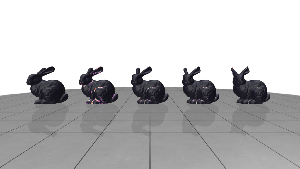
Table2: Curvature state transition in Algorithm 2
We evaluated the proposed 3D grid based algorithm on five models namely Cheburashka, Fandisk, Stanford-bunny, Homer, Suzanne. The optimal threshold epsilon was set to 0.1 and the penalty was fixed at 50. The table summrizes the before and after curvature counts with the algorithm run time.
| Model | Epsilon | Penalty | Flat Vertices (Before) | Non-Flat Vertices (Before) | Flat Vertices (After) | Non-Flat Vertices (After) | Flat Vertex Gain | Run time |
|---|---|---|---|---|---|---|---|---|
| Cheburashka | 0.1 | 50 | 6293 | 376 | 6411 | 258 | +118 | 308.198s |
| Fandisk | 0.1 | 50 | 6427 | 48 | 6429 | 46 | +2 | 58.310s |
| Stanford-bunny | 0.1 | 50 | 34071 | 540 | 34444 | 167 | +373 | 410.793s |
| Homer | 0.1 | 50 | 5313 | 689 | 5526 | 476 | +213 | 535.254s |
| Suzanne | 0.1 | 50 | 115 | 350 | 193 | 272 | +78 | 317.417s |
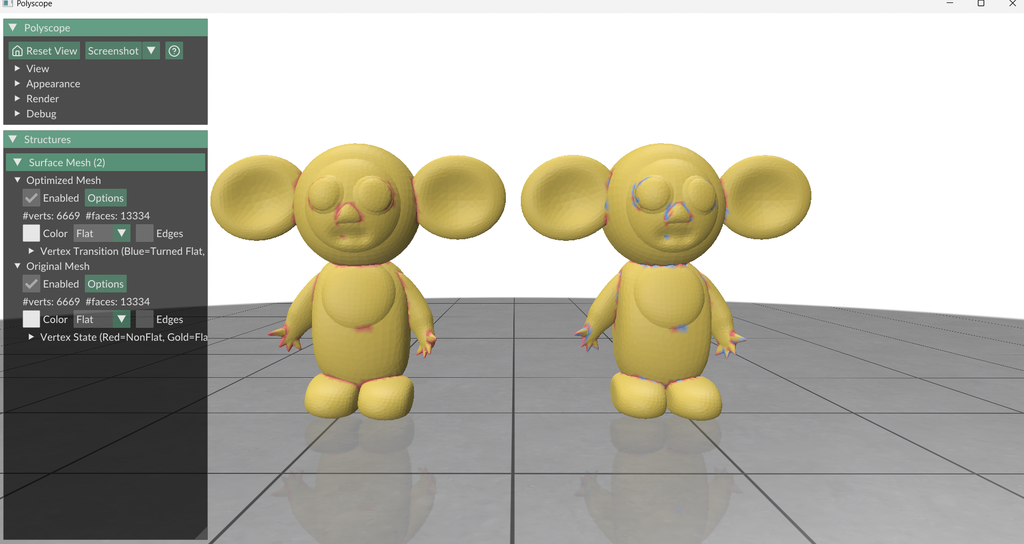
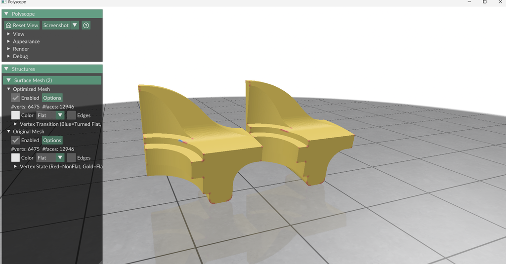
Table 3: Geometry preservation.
Normalized RMS displacement measures the overall surface change relative to the model size, while maximum edge change captures the worst local edge-length distortion. Minimum area ratio measures the strongest triangle compression, with values closer to one indicating better area preservation. Minimum triangle quality ranges from zero to one, where values near zero indicate thin or nearly degenerate triangles. Maximum normal change measures the largest local surface-orientation deviation, and the flipped-face count detects invalid face inversions.
| Family | Operator | Normalized RMS ↓ | Max edge change ↓ | Min area ratio ↑ | Min quality ↑ | Max normal change ↓ | Flipped faces |
|---|---|---|---|---|---|---|---|
| Vertex-based | Normal one-ring | 0.00569% | 24.71% | 0.304 | 0.00841 | 28.29° | 0 |
| Vertex-based | Double cone | 0.00373% | 19.14% | 0.313 | 0.01390 | 29.19° | 0 |
| Vertex-based | Virtual sphere | 0.00407% | 23.97% | 0.594 | 0.01390 | 73.81° | 0 |
| Grid-based | 3D grid | 0.01315% | 21.99% | 0.351 | 0.01392 | 30.00° | 0 |
Overall result:
The results indicate no operator dominates across all criteria. The double cone achieved the highest normalized RMS and maximum edge change, with a competitive minimum quality. The virtual sphere preserves triangle area best, but at the cost of a much larger maximum normal change. The normal one ring yields the smallest normal deviation but the lowest minimum quality and the largest edge change. The 3D grid is competitive in quality and normal change but has the highest RMS displacement. All the operators produced zero flipped faces.
Future directions:
- Extending these algorithm for real time use will likely require cost reduction strategies such as principal component analysis (PCA), proper orthogonal decomposition (POD).
- The evaluation covers geometric fidelity and mesh validity only. A systematic study of memory scaling and computational cost reduction strategies is a natural direction for future work.
- Testing on more complex models is needed to check the generalizability of the algorithms.
Reference:
- R. H. Byrd, P. Lu, J. Nocedal, and C. Zhu, A Limited Memory Algorithm for Bound Constrained Optimization, pp. 1190–1208, 1995. https://doi.org/10.1137/0916069
- L. Shapira, A. Shamir, and D. Cohen-Or, Consistent Mesh Partitioning and Skeletonisation using the Shape Diameter Function, vol. 24, no. 4, pp. 249–259, 2008. https://doi.org/10.1007/s00371-007-0197-5
- B. Keinert, M. Innmann, M. S\”anger, and M. Stamminger, Spherical Fibonacci Mapping, vol. 34, no. 6, article 193, 2015. https://doi.org/10.1145/2816795.2818131
- D. Zint, R. Grosso, and F. Lunz, “Discrete mesh optimization on surface and volume meshes,” in Proc. 28th Int. Meshing Roundtable (IMR), 2019, pp. 159–174.
- A. Nealen, T. Igarashi, O. Sorkine, and M. Alexa, “Laplacian mesh optimization,” in Proc. 4th Int. Conf. Computer Graphics and Interactive Techniques in Australasia and Southeast Asia (GRAPHITE ‘06), 2006, pp. 381–389.
