Categories
Research

3D Object Reconstruction using 2D Medial Axis

During Week 3, we had the incredible opportunity to dive into an amazing project on 3D object reconstruction using medial axis. This journey wouldn’t have been possible without the guidance of Professor Kathryn Leonard and Professor Geraldine Morin. They were truly wonderful advisors, offering us their insight and support every step of the way. We’re so excited to share our thoughts and results with you all! Let’s start with some basic background.

by Stephanie Jung, Evelyn Zhu and Anja Milutinović
  • What is a Medial axis ?

The medial axis is the “skeleton” of a shape. In 2D, the medial axis of a shape is the set of all points that are equidistant from at least two points on the boundary, i.e. the centers of the largest circles you can inscribe inside it. Paired with the radius at each point, it’s a compact yet near-complete description of a shape: sweeping those inscribed disks/balls back along the axis reproduces the original subject. For a straight rod, the medial axis is a line, for a bent tube it’s a curve, and for a torus it’s a circle. The axis really captures a shape’s essential structure in far fewer numbers than the full surface. 

One of the nice properties of the medial axis is that it preserves topology and geometry of the original shape. Given the medial axis of a 2D shape and the corresponding radius of each medial axis point, the original shape can be reconstructed.

  • How do we Compute Medial axis using Voronoi diagrams?

The medal axis is defined with respect to the continuous boundary of a shape and computing exact medial axis is then difficult. It’s then easier to approximate it using Voronoi diagrams of sample points on the boundary.

If we have a set of sample points P = {p1, p2, … , pn}, the Voronoi cell of the sample point pi is a set of all points that are closer to pi, then any other pj:

Vi={xn|xpixpj, j}V_i = \left\{ x \in \mathbb{R}^n \;\middle|\; \|x – p_i\| \le \|x – p_j\|,\ \forall j \right\}

The Voronoi diagram is a collection of all Voronoi cells.

The medial axis and Voronoi diagram’s edges both have in common that they are defined by points that are equidistant from multiple boundary locations. The algorithm to compute medal axis then becomes:

  1. Sample the boundary of the given object
  2. Construct the Voronoi diagram of the sample points
  3. Keep only the Voronoi vertices that are inside the object
  4. Connect the neighboring vertices with existing Voronoi edges
A visual example showing the medial axis of a 2D Baymax silhouette. This particular image actually shows a faulty medial axis. Based on the definition of medial axis, you can determine visually which branches should not be there.

With this foundational understanding of medial axes and Voronoi diagrams under our belts, we were ready to tackle the core of our Week 3 project. We wanted to see if we could take these 2D ‘skeletons’ and use them to solve a much more complex problem: bringing flat images to life by reconstructing a full 3D object from them.

Reconstructing 3d object from its 2d images using medial axis

Method 1:

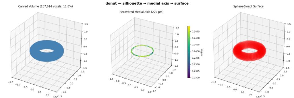
  • We reconstruct a 3D object from a set of binary silhouettes taken from viewpoints spread over a sphere. For each view we compute an orthographic projection of the mesh to get a silhouette, then extract its 2D medial axis and radius via the Voronoi diagram of the boundary. We then fuse the views in 3D by carving a voxel grid (keeping only voxels whose projection lands inside every silhouette) and thin the result with a 3D skeletonization to recover the object’s 3D medial axis. Finally, we rebuild the surface by sweeping balls of the recovered radius along that axis, which reproduces the original shape. 

Pipeline Visualization:

Method 2:

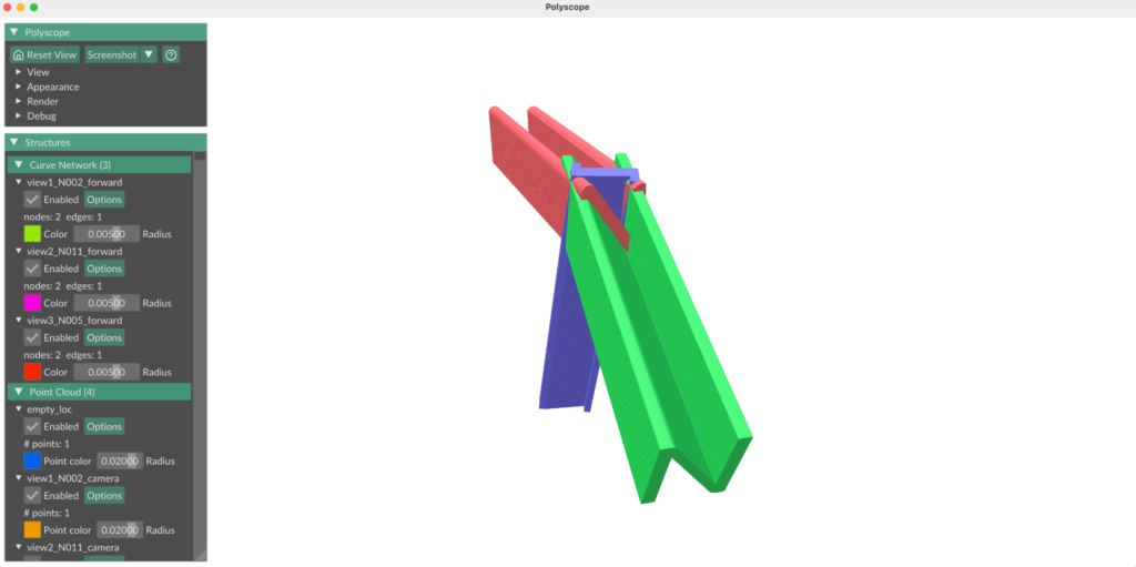
  • Each point on a 2D medial axis represents the center of a maximal inscribed circle. All of the possible centers lie along the camera’s viewing direction. So then, every circle naturally defines a cylinder in 3D space whose axis is the same direction as the camera viewing direction and whose radius equals the radius of the medial circle. Each orthographic image generates an entire set of cylinders, or as we called them “swept cylinders”.
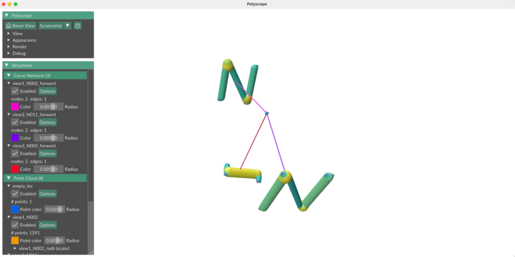
  • We position the “swept cylinders” by setting the medial axis from each camera view in a world space and using the camera parameters (orthographic scale, location with respect to the object, viewing direction) to position each 2D medial axis about the world origin such that it reflected the camera view about the original 3D object. 
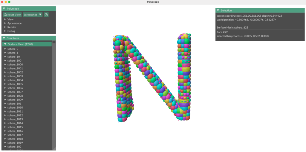
N model: Medial axes from 3 different camera views, projected into a world space. Line propagating from the center of each camera view indicates camera forward direction. Blue point (where all camera forwards intersect) indicates the point all cameras were focused on (center of the original 3D object).
N model: Visualization of swept cylinders.

Intersecting the “sweep cylinders” from multiple views in 3D space, gives us a feasible reconstruction region:

Ω=swept cylinders(cylinders in swept cylinderC)\Omega = \bigcap_{\text{swept cylinders}} \left( \bigcup_{\text{cylinders in swept cylinder}} C \right)

Method 2a:

To compute the radii of each sphere we use a signed distance function for a cylinder. Since the center point can belong to multiple cylinders, in each “swept cylinder”, we take the one where the point has a maximum SDF. The sphere must be contained in the intersection of each chosen “swept cylinder”, so the final radius is taken as minimum.

R(p)=minswept cylinders(maxcylinders in swept cylinderSDF(c,p))R(p)=\min_{\text{swept cylinders}} \left( \max_{\text{cylinders in swept cylinder}} \operatorname{SDF}(c,p) \right)
One of the view of the object with it’s 2d medial axis
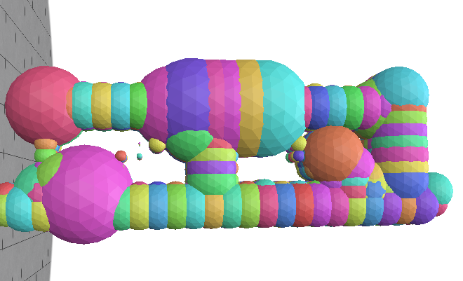
Reconstruction using maximal spheres with sampled sphere centers

Method 2b:

In an alternative method, to compute the radii of each sphere we use the signed distance field of the binary image for each view, which evaluates a point’s distance from the nearest boundary of the shape. We sample points in 3D space at regular intervals and project them down into each view’s 2D image plane, then compute the signed distance for the point in that view. This method is functionally equivalent to using a 3D signed distance field in world space; it evaluates a point’s distance from the nearest boundary of the swept cylinder for that camera view. Then, the radius of a sphere centered at a point is the minimum signed distance across all camera views, since the sphere must be contained in the intersection of all swept cylinders.

N model (3D)
N model: binary image of the N model from one camera view
N model: Reconstruction of N model, from images taken from 3 different camera views

Categories
Research

Geometric Deep Learning for Fluids

SGI Mentor: Akhil Sadam

SGI Fellows: Santoshi Yadagiri, Pietro Palombini

1. Introduction

Many geophysical inverse problems require reconstruction of a high-dimensional physical state from observations that are incomplete, noisy, or available only over part of the spatial domain. In oceanic and atmospheric applications, observations may be coarse, sparse, or separated by large unmeasured regions. The objective is not only to produce a plausible reconstruction, but also to characterize how much information the measurements provide about the unobserved portion of the state.

Let the clean physical state be partitioned as

U0=(CD),U_0 = \begin{pmatrix} C\\ D \end{pmatrix},

where CC denotes the observed or near component and DD denotes the unobserved or far component. Measurements are assumed to depend directly only on CC

Y=AC+N,N𝒩(0,R).Y = AC+N, \qquad N\sim\mathcal{N}(0,R).

Equivalently, defining

H=(Aamp;0),H = \begin{pmatrix} A&0 \end{pmatrix},

the observation model becomes

Y=HU0+N.Y = HU_0+N.

The operator AA determines which spatial directions or scales of the near state are measured, while RR describes the measurement-noise covariance. No component of DD is observed directly. Information about the far region can therefore be recovered only through statistical or dynamical coupling between CC and DD.

This problem is motivated by the reconstruction of quasi-geostrophic flow fields from coarse, sparse, and gappy observations. Diffusion-based generative models can provide probabilistic reconstructions without explicitly solving for a single deterministic inverse. However, recent numerical results show that guided unconditional methods such as diffusion posterior sampling may have difficulty propagating observational information into unobserved regions [11]. This raises the question of how information from a partial observation influences uncertainty and reconstruction quality outside the observed region.

First, a linear Gaussian model is used to derive the conditional distribution, uncertainty reduction, and information transfer exactly. Second, the same structure is extended to a nonlinear flow-matching model through local linearization of the denoising map and the guided velocity field.

2. Background

2.1 Geophysical Inverse Problems

An inverse problem seeks to infer an unknown physical state from indirect measurements. In the present setting, the forward observation process maps the clean state U0U_0 to data YY:

Y=𝒜(U0)+N.Y = \mathcal{A}(U_0)+N.

For a linear observation operator, this reduces to

Y=HU0+N.Y = HU_0+N.

The inverse problem is generally ill posed because multiple clean states may produce similar observations, particularly when the data are low resolution, spatially incomplete, or noisy. Rather than selecting a single reconstruction, a probabilistic method seeks the posterior distribution

p(U0|Y=y).p(U_0\mid Y=y).

This posterior represents both the states that are compatible with the measurement and the remaining uncertainty after conditioning.

In the near-far decomposition, the corresponding far-state posterior is

p(D|Y=y).p(D\mid Y=y).

A principal objective is to determine when this distribution differs meaningfully from the prior distribution of DD. If it does not, then the observation provides no usable information about the unobserved region.

2.2 Diffusion-Based Posterior Sampling

Diffusion models introduce a family of noisy states connecting clean data to an approximately Gaussian terminal distribution. A standard linear forward-noising model is

Ut=αtU0+σtε,ε𝒩(0,In).U_t = \alpha_tU_0+\sigma_t\varepsilon, \qquad \varepsilon\sim\mathcal{N}(0,I_n).

The reverse process is governed by a score function. The unconditional score is

st(u)=ulogpt(u),s_t(u) = \nabla_u\log p_t(u),

while the conditional score is

st(u,y)=ulogpt(u|y).s_t^\ast(u,y) = \nabla_u\log p_t(u\mid y).

Bayes’ rule gives the score decomposition

st(u,y)=st(u)+ulogpt(y|u).s_t^\ast(u,y) = s_t(u) + \nabla_u\log p_t(y\mid u).

The first term is given by an unconditional generative model. The second term incorporates the measurement and directs sampling toward states that are compatible with the observation.

The likelihood term is usually intractable because the observation is defined on the clean state U0U_0, while the reverse process evolves through the noisy state UtU_t. Diffusion posterior sampling approximates this term by applying the observation operator to a denoised estimate of the clean state and differentiating the resulting data-fidelity loss [22].

2.3 QG Sampler and Observation Operator

The quasi-geostrophic (QG) implementation provides a concrete realization of the likelihood-guided reverse process. The sampler assumes a variance-preserving stochastic differential equation and supports unconditional sampling, conditional sampling, classifier-free guidance, SDEdit, and diffusion posterior sampling [33].

At diffusion time tt, the unconditional network predicts a noise field

εθ(Ut,t).\varepsilon_\theta(U_t,t).

Using the variance-preserving parameterization, the corresponding estimate of the clean field is

U^0(Ut,t)=1μt(Utσtεθ(Ut,t)).\widehat{U}_0(U_t,t) = \frac{1}{\mu_t} \left( U_t-\sigma_t\varepsilon_\theta(U_t,t) \right).

The implementation then applies a low-resolution observation operator to this clean-state estimate. In Fourier space, the field I first multiplied by a Gaussian filter of the form

G(k)=exp[4kr2(sΔx)224],G(k) = \exp \left[ -\frac{4k_r^2(s\Delta x)^2}{24} \right],

where ss is the coarsening scale, Δx\Delta x is the grid spacing, and krk_r is the radial wavenumber. Additional spectral cutoffs remove modes above the coarse-grid Nyquist limit. The filtered field is transformed back to physical space, average pooled on an s×ss\times s grid, and repeated to the original resolution.

The resulting operator may be represented abstractly as

𝒜LES(U^0).\mathcal{A}_{\mathrm{LES}} \left( \widehat{U}_0 \right).

The implementation also includes an optional gappy-observation mask that sets selected spatial swaths of the coarsened field to zero [33].

This construction makes the spatial bandwidth of the observation operator explicit. The Gaussian spectral filer, hard spectral cutoff, pooling scale, and spatial mask collectively determine which directions of the high-resolution state are visible to the likelihood.

2.4 Observation Support and Information Propagation

For a partial observation,

H=(Aamp;0),H = \begin{pmatrix} A&0 \end{pmatrix},

so the likelihood depends directly only on the near component. The spatial support of bandwidth of the observation kernel is encoded by AA. A wider kernel may observe more spatial directions, while a restricted kernel may leave large subspaces unmeasured.

Direct observation is not the only mechanism through which information can propagate. If the near and far components are statistically correlated, observing CC can reduce uncertainty in DD. In a nonlinear generative model, an analogous effect occurs when the predicted observed region depends on the hidden coordinates of the current state. The linear Gaussian model isolates this mechanism in a form that can be derived exactly.

3. Linear Gaussian Model

3.1 State and Observation Model

Let

U0=(CD)n,n=nC+nD,U_0 = \begin{pmatrix} C\\ D \end{pmatrix} \in\mathbb{R}^{n}, \qquad n=n_C+n_D,

with

CnC,DnD.C\in\mathbb{R}^{n_C}, \qquad D\in\mathbb{R}^{n_D}.

Assume a centered Gaussian prior

U0𝒩(0,Σ),U_0 \sim \mathcal{N}(0,\Sigma),

with block covariance

Σ=(ΣCCamp;ΣCDΣDCamp;ΣDD)0.\Sigma = \begin{pmatrix} \Sigma_{CC}&\Sigma_{CD}\\ \Sigma_{DC}&\Sigma_{DD} \end{pmatrix} \succ0.

The diagonal blocks are the marginal covariances

ΣCC=Cov(C),ΣDD=Cov(D),\Sigma_{CC} = \operatorname{Cov}(C), \qquad \Sigma_{DD} = \operatorname{Cov}(D),

and the off-diagonal blocks are the cross-covariances

ΣCD=Cov(C,D),ΣDC=ΣCD.\Sigma_{CD} = \operatorname{Cov}(C,D), \qquad \Sigma_{DC} = \Sigma_{CD}^{\top}.

The observation is

Y=AC+N,Am×nC,Y = AC+N, \qquad A\in\mathbb{R}^{m\times n_C},

where

N𝒩(0,R),R0,N \sim \mathcal{N}(0,R), \qquad R\succ0,

and NN is independent of U0U_0. With

H=(Aamp;0)m×n,H = \begin{pmatrix} A&0 \end{pmatrix} \in\mathbb{R}^{m\times n},

the observation equation is

Y=HU0+N.Y = HU_0+N.

3.2 Gaussian Conditioning

The conditioning calculation uses the following standard result. Let XX and ZZ be jointly Gaussian with zero means,

Cov(X)=SX,Cov(Z)=SZ0,Cov(X,Z)=SXZ.\operatorname{Cov}(X)=S_X, \qquad \operatorname{Cov}(Z)=S_Z\succ0, \qquad \operatorname{Cov}(X,Z)=S_{XZ}.

Then [44]

X|Z=z𝒩(SXZSZ1z,SXSXZSZ1SXZ).X\mid Z=z \sim \mathcal{N} \left( S_{XZ}S_Z^{-1}z, S_X-S_{XZ}S_Z^{-1}S_{XZ}^{\top} \right).

Because YY is a linear function of independent Gaussian variables, the pair (U0,Y)(U_0,Y) is jointly Gaussian. Its observation covariance is

SY:=Cov(Y)=HΣH+R=AΣCCA+R,S_Y := \operatorname{Cov}(Y) = H\Sigma H^\top+R = A\Sigma_{CC}A^\top+R,

and the state-observation cross-covariance is

Cov(U0,Y)=ΣH.\operatorname{Cov}(U_0,Y) = \Sigma H^\top.

Applying the Gaussian conditioning formula [44] gives

U0|Y=y𝒩(m0|y,Σ0|Y),U_0\mid Y=y \sim \mathcal{N} \left( m_{0\mid y}, \Sigma_{0\mid Y} \right),

where

m0|y=ΣHSY1ym_{0\mid y} = \Sigma H^\top S_Y^{-1}y

and

Σ0|Y=ΣΣHSY1HΣ.\Sigma_{0\mid Y} = \Sigma – \Sigma H^\top S_Y^{-1}H\Sigma.

The posterior mean depends linearly on the realized observation yy. The posterior covariance does not depend on the particular observed value because the model is linear Gaussian.

4. Information Transfer from C to D

4.1 Far-State Posterior

The cross-covariance between the far state and the observation is

Cov(D,Y)=ΣDCA.\operatorname{Cov}(D,Y) = \Sigma_{DC}A^\top.

Applying Gaussian conditioning directly to (D,Y)(D,Y) gives

D|Y=y𝒩(mD|y,ΣD|Y),D\mid Y=y \sim \mathcal{N} \left( m_{D\mid y}, \Sigma_{D\mid Y} \right),

with posterior mean

mD|y=ΣDCASY1ym_{D\mid y} = \Sigma_{DC}A^\top S_Y^{-1}y

and posterior covariance

ΣD|Y=ΣDDΣDCASY1AΣCD.\Sigma_{D\mid Y} = \Sigma_{DD} – \Sigma_{DC}A^\top S_Y^{-1}A\Sigma_{CD}.

These expressions separate the two mechanism that determine information transfer. The observation operator AA selects directions of the near state, while the cross-covariance ΣDC\Sigma_{DC} determines which of those observed directions are correlated with the far state.

If

ΣDCA=0,\Sigma_{DC}A^\top = 0,

then

mD|y=0,ΣD|Y=ΣDD.m_{D\mid y} = 0, \qquad \Sigma_{D\mid Y} = \Sigma_{DD}.

In this case, conditioning on the observation does not change the distribution of DD.

4.2 Reduction in Far-State Uncertainty

Define

QD=ΣDCASY1AΣCD.Q_D = \Sigma_{DC}A^\top S_Y^{-1}A\Sigma_{CD}.

Then

ΣD|Y=ΣDDQD.\Sigma_{D\mid Y} = \Sigma_{DD}-Q_D.

For any vnDv\in\mathbb{R}^{n_D},

vQDv=(AΣCDv)SY1(AΣCDv)0.v^\top Q_Dv = \left(A\Sigma_{CD}v\right)^\top S_Y^{-1} \left(A\Sigma_{CD}v\right) \geq0.

Therefore,

QD0Q_D\succeq0

and

ΣD|YΣDD.\Sigma_{D\mid Y} \preceq \Sigma_{DD}.

Thus, conditioning cannot increase posterior uncertainty in any linear direction of the far state.

Let

LD=ΣDCA.L_D = \Sigma_{DC}A^\top.

Since

QD=LDSY1LD,Q_D = L_DS_Y^{-1}L_D^\top,

the rank of the covariance reduction satisfies

rank(QD)=rank(LD)rank(A)m.\operatorname{rank}(Q_D) = \operatorname{rank}(L_D) \leq \operatorname{rank}(A) \leq m.

Consequently, mm measurements can reduce far-state uncertainty in at most mm independent directions. In addition,

mD|yRange(LD).m_{D\mid y} \in \operatorname{Range}(L_D).

Both the posterior-mean update and covariance reduction are therefore restricted to directions selected by ΣDCA\Sigma_{DC}A^\top.

4.3 Mutual Information

For a Gaussian random variable XkX\in\mathbb{R}^k with covariance S0S\succ0, the differential entropy is

h(X)=12log((2πe)kdetS).h(X) = \frac{1}{2} \log \left( (2\pi e)^k\det S \right).

Applying

I(D;Y)=h(D)h(D|Y)I(D;Y) = h(D)-h(D\mid Y)

causes the constant terms to cancel and gives the determinant ratio below.

The reduction in uncertainty can also be expressed through mutual information. For Gaussian variables.

I(D;Y)=12logdetΣDDdetΣD|Y.I(D;Y) = \frac{1}{2} \log \frac{\det\Sigma_{DD}} {\det\Sigma_{D\mid Y}}.

This quantity measures the information about the far state contained in the observation. It vanishes exactly when

ΣDCA=0.\Sigma_{DC}A^\top = 0.

Therefore, the observation carries information about DD only through the near-far covariance directions that are also visible to AA.

Define the normalized covariance reduction

KD=ΣDD1/2QDΣDD1/2.K_D = \Sigma_{DD}^{-1/2} Q_D \Sigma_{DD}^{-1/2}.

Then

ΣD|Y=ΣDD1/2(IKD)ΣDD1/2,\Sigma_{D\mid Y} = \Sigma_{DD}^{1/2} \left(I-K_D\right) \Sigma_{DD}^{1/2},

and

I(D;Y)=12logdet(IKD).I(D;Y) = -\frac{1}{2} \log\det\left(I-K_D\right).

The eigenvalues of KDK_D quantify the fractional uncertainty reduction along informative far-state directions.

4.4 Information Under Forward Noising

For the forward-noised far state

Dt=αtD+σtεD,D_t = \alpha_tD+\sigma_t\varepsilon_D,

the unconditional and conditional covariances are

Cov(Dt)=αt2ΣDD+σt2InD\operatorname{Cov}(D_t) = \alpha_t^2\Sigma_{DD} + \sigma_t^2I_{n_D}

and

Cov(Dt|Y)=αt2ΣD|Y+σt2InD.\operatorname{Cov}(D_t\mid Y) = \alpha_t^2\Sigma_{D\mid Y} + \sigma_t^2I_{n_D}.

Hence,

I(Dt;Y)=12logdet(αt2ΣDD+σt2InD)det(αt2ΣD|Y+σt2InD).I(D_t;Y) = \frac{1}{2} \log \frac{ \det\left( \alpha_t^2\Sigma_{DD} + \sigma_t^2I_{n_D} \right) }{ \det\left( \alpha_t^2\Sigma_{D\mid Y} + \sigma_t^2I_{n_D} \right) }.

For σt>0\sigma_t>0, define the signal-to-noise ratio

λt=αt2σt2.\lambda_t = \frac{\alpha_t^2}{\sigma_t^2}.

Scaling by a nonzero constant preserves mutual information, so

I(Dt;Y)=I(λtD+εD;Y).I(D_t;Y) = I \left( \sqrt{\lambda_t}D+\varepsilon_D; Y \right).

To compare two signal-to-noise ratios, suppose

λ1λ20\lambda_1\geq\lambda_2\geq0

and define

a=λ2λ1,a = \sqrt{ \frac{\lambda_2}{\lambda_1} },
Z1=λ1D+ε1.Z_1 = \sqrt{\lambda_1}D+\varepsilon_1.

Let

Z2=aZ1+1a2ε,Z_2 = aZ_1 + \sqrt{1-a^2}\, \varepsilon’,

where ε1\varepsilon_1 and ε\varepsilon’ are independent standard Gaussian variables independent of (D,Y)(D,Y). Expanding Z2Z_2 gives

Z2=λ2D+(aε1+1a2ε).Z_2 = \sqrt{\lambda_2}D + \left( a\varepsilon_1 + \sqrt{1-a^2}\, \varepsilon’ \right).

The Gaussian noise in parentheses is standard, so Z2Z_2 has the lower-signal-to-noise law and is obtained from Z1Z_1 by adding noise. Therefore,

YZ1Z2Y \longrightarrow Z_1 \longrightarrow Z_2

is a Markov chain. By the data-processing inequality [5],

I(Z2;Y)I(Z1;Y).I(Z_2;Y) \leq I(Z_1;Y).

Hence I(Dt;Y)I(D_t;Y) is nondecreasing in λt=αt2/σt2\lambda_t=\alpha_t^2/\sigma_t^2. Equivalently, forward noising cannot increase the information about YY available in the far state. This gives an information-theoretic interpretation of the reverse process. As the signal-t0-noise ratio increases, the process can progressively recover the information present in the conditional clean-state distribution.

5. Gaussian Score and DPS

5.1 Forward-Noised Posterior

The forward-noised state is

Ut=αtU0+σtε,ε𝒩(0,In),U_t = \alpha_tU_0+\sigma_t\varepsilon, \qquad \varepsilon\sim\mathcal{N}(0,I_n),

with independent of (U0,Y)(U_0,Y). Since U0|Y=yU_0\mid Y=y is Gaussian,

Ut|Y=y𝒩(αtm0|y,αt2Σ0|Y+σt2In).U_t\mid Y=y \sim \mathcal{N} \left( \alpha_tm_{0\mid y}, \alpha_t^2\Sigma_{0\mid Y} + \sigma_t^2I_n \right).

The far marginal satisfies

Dt|Y=y𝒩(αtmD|y,αt2ΣD|Y+σt2InD).D_t\mid Y=y \sim \mathcal{N} \left( \alpha_tm_{D\mid y}, \alpha_t^2\Sigma_{D\mid Y} + \sigma_t^2I_{n_D} \right).

5.2 Exact Conditional Score

For a Gaussian random variable

X𝒩(m,S),X\sim\mathcal{N}(m,S),

the score is

xlogpX(x)=S1(xm).\nabla_x\log p_X(x) = -S^{-1}(x-m).

Applying this identity to the conditional distribution of UtU_t gives

st(u,y)=(αt2Σ0|Y+σt2In)1(uαtm0|y).s_t^\ast(u,y) = – \left( \alpha_t^2\Sigma_{0\mid Y} + \sigma_t^2I_n \right)^{-1} \left( u-\alpha_tm_{0\mid y} \right).

Unconditionally,

Ut𝒩(0,St),U_t \sim \mathcal{N}(0,S_t),

where

St=αt2Σ+σt2In.S_t = \alpha_t^2\Sigma+\sigma_t^2I_n.

The unconditional score is therefore

st(u)=St1u.s_t(u) = -S_t^{-1}u.

The score of the far marginal is

dlogptD(d|y)=(αt2ΣD|Y+σt2InD)1(dαtmD|y).\nabla_d\log p_t^D(d\mid y) = – \left( \alpha_t^2\Sigma_{D\mid Y} + \sigma_t^2I_{n_D} \right)^{-1} \left( d-\alpha_tm_{D\mid y} \right).

This far-marginal score is not generally equal to the far coordinates of the full-state score. The full-state score may depend jointly on the current near and far coordinates, while the marginal score depends only on dd.

5.3 Exact Denoiser and Noisy Likelihood

The pair (U0,Ut)(U_0,U_t) is jointly Gaussian, with

Cov(U0,Ut)=αtΣ\operatorname{Cov}(U_0,U_t) = \alpha_t\Sigma

and

Cov(Ut)=St.\operatorname{Cov}(U_t) = S_t.

Conditioning gives

U0|Ut=u𝒩(Btu,Σ0|t),U_0\mid U_t=u \sim \mathcal{N} \left( B_tu, \Sigma_{0\mid t} \right),

where

Bt=αtΣSt1B_t = \alpha_t\Sigma S_t^{-1}

and

Σ0|t=Σαt2ΣSt1Σ.\Sigma_{0\mid t} = \Sigma – \alpha_t^2 \Sigma S_t^{-1}\Sigma.

The exact unconditional denoiser is therefore

𝔼[U0|Ut=u]=Btu.\mathbb{E}[U_0\mid U_t=u] = B_tu.

Given Ut=uU_t=u, the observation distribution is

Y|Ut=u𝒩(HBtu,Γt),Y\mid U_t=u \sim \mathcal{N} \left( HB_tu, \Gamma_t \right),

where

Γt=R+HΣ0|tH.\Gamma_t = R + H\Sigma_{0\mid t}H^\top.

The matrix Γt\Gamma_t is the effective observation covariance at time tt. It combines the original measurement noise with the remaining uncertainty about the clean state after conditioning on Ut=uU_t=u.

Differentiating the exact noisy likelihood gives

ulogpt(y|u)=BtHΓt1(yHBtu).\nabla_u\log p_t(y\mid u) = B_t^\top H^\top\Gamma_t^{-1} \left( y-HB_tu \right).

5.4 Exact Gaussian DPS Identity

Combining the unconditional score with the noisy likelihood gradient yields

st(u,y)=st(u)+BtHΓt1(yHBtu).s_t^\ast(u,y) = s_t(u) + B_t^\top H^\top\Gamma_t^{-1} \left( y-HB_tu \right).

In the linear Gaussian model, this identity is exact. It has the same structure as diffusion posterior sampling:

  1. estimate the clean state from the current noisy state
  2. apply the observation operator to the estimate
  3. compute the measurement residual
  4. propagate the residual back to the current state.

A standard point-estimate DPS approximation replaces the effective covariance Γt\Gamma_t with a simpler measurement weighting and replaces the exact linear denoiser BtuB_tu with a learned denoising estimate. The Gaussian analysis therefore provides both an exact benchmark and a direct motivation for the nonlinear flow-matching extension.

5.5 Exact Reverse-Process Distribution

Let U^\widehat{U} denote the output of the exact continous reverse process initialized from the exact terminal distribution, driven by the exact conditional score, and simulated without numerical error. Because this is the exact reverse process,

P(U^|Y=y)=P(U0|Y=y).P \left( \widehat{U}\mid Y=y \right) = P \left( U_0\mid Y=y \right).

In the linear Gaussian setting, this gives

U^|Y=y𝒩(m0|y,Σ0|Y).\widehat{U}\mid Y=y \sim \mathcal{N} \left( m_{0\mid y}, \Sigma_{0\mid Y} \right).

Let PDP_D denote projection onto the far-state coordinates and define

D^=PDU^.\widehat{D} = P_D\widehat{U}.

Then

D^|Y=y𝒩(mD|y,ΣD|Y).\widehat{D}\mid Y=y \sim \mathcal{N} \left( m_{D\mid y}, \Sigma_{D\mid Y} \right).

Thus, under exact sampling assumptions, the reverse process reproduces both the complete conditional distribution and its far-state marginal.

5.6 Relation to the QG DPS Implementation

The exact Gaussian identity can be compared directly with the quasi-geostrophic sampler. The exact linear denoiser

BtuB_tu

is replaced by the learned clean-state estimate

U^0(Ut,t)=1μt(Utσtεθ(Ut,t)).\widehat{U}_0(U_t,t) = \frac{1}{\mu_t} \left( U_t-\sigma_t\varepsilon_\theta(U_t,t) \right).

The theoretical observation operator HH is replaced by the filtered and coarsened operator

𝒜LES.\mathcal{A}_{\mathrm{LES}}.

The implementation defines a mean-squared measurement loss

meas(Ut)=MSE(𝒜LES(U^0(Ut,t)),y).\mathcal{L}_{\mathrm{meas}}(U_t) = \operatorname{MSE} \left( \mathcal{A}_{\mathrm{LES}} \left( \widehat{U}_0(U_t,t) \right), y \right).

Automatic differentiation is used to compute

Utmeas(Ut).\nabla_{U_t} \mathcal{L}_{\mathrm{meas}}(U_t).

The implemented DPS correction is

gtDPS=12σscaledUtmeas(Ut),g_t^{\mathrm{DPS}} = -\frac{1}{2\sigma_{\mathrm{scaled}}} \nabla_{U_t} \mathcal{L}_{\mathrm{meas}}(U_t),

with time-dependent scale

σscaled=σmeasure2+CDPS(σtμt)2.\sigma_{\mathrm{scaled}} = \sigma_{\mathrm{measure}}^2 + C_{\mathrm{DPS}} \left( \frac{\sigma_t}{\mu_t} \right)^2.

The correction is added to the model score during both the reverse updated and the Langevin correction steps [3].

This implementation has the same computational structure as the exact Gaussian likelihood correction:

  1. estimate the clean state from the current noisy state
  2. apply a measurement operator to the estimate
  3. compare the predicted measurement with the observed field
  4. differentiate the discrepancy with respect to the current state
  5. add the resulting correction to the unconditional score

The principal difference is the likelihood weighting. In the exact Gaussian model, the residual is weighted by the full effective covariance

Γt1=(R+HΣ0|tH)1.\Gamma_t^{-1} = \left( R+H\Sigma_{0\mid t}H^\top \right)^{-1}.

The implementation instead uses the scalar factor

1σscaled\frac{1}{\sigma_{\mathrm{scaled}}}

Thus, the Gaussian calculation identifies the matrix-valued uncertainty correction that is approximated in practice by a time-dependent scalar weighting. It also clarifies how the observation operator’s spectral bandwidth and spatial mask determine which state-space directions receive guidance.

6. Flow-Matching Extension

The linear Gaussian model provides an exact setting in which the posterior distribution and conditional likelihood gradient can be computed analytically. The clean-state estimator is linear, and the noisy likelihood gradient takes the form

ulogpt(y|u)=BtHΓt1(yHBtu),\nabla_u \log p_t(y\mid u) = B_t^\top H^\top \Gamma_t^{-1} \left(y-HB_tu\right),

where BtuB_tu is the conditional estimate of the clean state and Γt\Gamma_t accounts for measurement noise and the remaining uncertainty in that estimate.

The same structure can be extended to a nonlinear flow-matching model by replacing the linear clean-state estimator with a time dependent denoising map.

6.1 Denoising Map

Let UtnU_t\in\mathbb{R}^n denote the state at time tt. The unconditional flow is controlled by

dUtdt=vt(Ut),\frac{dU_t}{dt}=v_t(U_t),

where vt:nnv_t:\mathbb{R}^n\rightarrow\mathbb{R}^n is the unconditional velocity field.

Assume that a time-dependent map FtF_t predicts the clean state U0U_0 from the current state

U^0=Ft(Ut).\widehat{U}_0=F_t(U_t).

The map FtF_t is treated as given. No separate differential equation for FtF_t is introduced.

The observation model is

Y=HU0+N,N𝒩(0,R),Y=HU_0+N, \qquad N\sim\mathcal{N}(0,R),

where HH is the observation operator and R0R\succ0 is the measurement-noise covariance.

Applying the observation operator to the predicted clean state gives the predicted measurement

Y^t=HFt(Ut).\widehat{Y}_t=HF_t(U_t).

The corresponding measurement residual is

rt(Ut)=yHFt(Ut).r_t(U_t)=y-HF_t(U_t).

This residual measures the disagreement between the observed data and the observation predicted from the current state.

6.2 DPS Guidance

Diffusion posterior sampling introduces an observation-dependent correction through the gradient of the likelihood. Using Ft(Ut)F_t(U_t) as a point estimate of the clean state, the Gaussian likelihood is

p(y|Ft(Ut))exp[12(yHFt(Ut))R1(yHFt(Ut))]p\bigl(y\mid F_t(U_t)\bigr) \propto \exp\left[ -\frac{1}{2} \left(y-HF_t(U_t)\right)^\top R^{-1} \left(y-HF_t(U_t)\right) \right]

The DPS guidance term is defined as

gt(Ut,y)=λtUtlogp(y|Ft(Ut)),g_t(U_t,y) = \lambda_t \nabla_{U_t} \log p\bigl(y\mid F_t(U_t)\bigr),

where λt\lambda_t controls the time-dependent strength and sign convention of the guidance.

Define the Jacobian of FtF_t by

JFt(Ut)=Ft(Ut)Ut.J_{F_t}(U_t) = \frac{\partial F_t(U_t)}{\partial U_t}.

Applying the chain rule gives

gt(Ut,y)=λtJFt(Ut)HR1[yHFt(Ut)].g_t(U_t,y) = \lambda_t J_{F_t}(U_t)^\top H^\top R^{-1} \left[ y-HF_t(U_t) \right].

Equivalently,

gt(Ut,y)=λt2UtyHFt(Ut)R12,g_t(U_t,y) = -\frac{\lambda_t}{2} \nabla_{U_t} \left\| y-HF_t(U_t) \right\|_{R^{-1}}^2,

where

zR12=zR1z.\|z\|_{R^{-1}}^2 = z^\top R^{-1}z.

The residual is evaluated in observation space. Multiplication by HH^\topmaps it to the clean-state space, while JFt(Ut)J_{F_t}(U_t)^\toppropogates the correction from the predicted clean state back to the current state.

Although the measurement is defined on U0U_0, the likelihood gradient can guide intermediate states throughout the flow.

6.3 Guided Flow

After adding the DPS correction, the state evolves according to

dUtdt=vt(Ut)+gt(Ut,y).\frac{dU_t}{dt} = v_t(U_t)+g_t(U_t,y).

Define the full guided velocity as

ft(U,y)=vt(U)+gt(U,y).f_t(U,y)=v_t(U)+g_t(U,y).

The guided dynamics are therefore

dUtdt=ft(Ut,y).\frac{dU_t}{dt}=f_t(U_t,y).

The complete observation-guided update follows the sequence

UtFt(Ut)HFt(Ut)gt(Ut,y).U_t \longrightarrow F_t(U_t) \longrightarrow HF_t(U_t) \longrightarrow g_t(U_t,y).

The current state is first mapped to a clean-state prediction. This prediction is passed through the observation operator, and the resulting residual is propagated back through the denoising map.

7. Moment Evolution

The DPS equation describes the evolution of an individual trajectory. To characterize the conditional distribution of trajectories given Y=yY=y, consider the conditional mean and covariance.

7.1 Conditional Mean

Define the conditional mean as

mt=𝔼[Ut|Y=y].m_t = \mathbb{E}[U_t\mid Y=y].

Since each trajectory satisfies

U˙t=ft(Ut,y),\dot{U}_t=f_t(U_t,y),

differentiating the conditional expectation gives

m˙t=𝔼[ft(Ut,y)|Y=y].\dot{m}_t = \mathbb{E} \left[ f_t(U_t,y)\mid Y=y \right].

Substituting the definition of the guided velocity yields

m˙t=𝔼[amp;vt(Ut)amp;+λtJFt(Ut)HR1(yHFt(Ut))|Y=y].\begin{aligned} \dot{m}_t = \mathbb{E}\Big[ & v_t(U_t)\\ &+ \lambda_t J_{F_t}(U_t)^\top H^\top R^{-1} \left( y-HF_t(U_t) \right) \;\Big|\;Y=y \Big]. \end{aligned}

When either vtv_t or FtF_t is nonlinear, the expectation depends on the full conditional distribution of UtU_t, rather than only on mtm_t. The mean equation is there not closed in general.

7.2 Conditional Covariance

Define the conditional covariance by

Σt=Cov(Ut|Y=y).\Sigma_t = \operatorname{Cov}(U_t\mid Y=y).

Equivalently,

Σt=𝔼[(Utmt)(Utmt)|Y=y].\Sigma_t = \mathbb{E} \left[ (U_t-m_t)(U_t-m_t)^\top \mid Y=y \right].

Let

δUt=Utmt.\delta U_t=U_t-m_t.

Then

δU˙t=ft(Ut,y)m˙t.\dot{\delta U}_t = f_t(U_t,y)-\dot{m}_t.

Differentiating

Σt=𝔼[δUtδUt|Y=y]\Sigma_t = \mathbb{E} \left[ \delta U_t\delta U_t^\top \mid Y=y \right]

gives

Σ˙t=𝔼[amp;(ft(Ut,y)m˙t)(Utmt)amp;+(Utmt)(ft(Ut,y)m˙t)|Y=y].\begin{aligned} \dot{\Sigma}_t = \mathbb{E}\Big[ & \left( f_t(U_t,y)-\dot{m}_t \right) (U_t-m_t)^\top\\ &+ (U_t-m_t) \left( f_t(U_t,y)-\dot{m}_t \right)^\top \mid Y=y \Big]. \end{aligned}

This covariance equation is also exact, but it is not closed for a nonlinear guided velocity field.

The flow-matching dynamics considered here are deterministic. Consequently, there is no separate process-noise covariance term. The conditional covariance instead comes from the distribution of the initial state and from conditioning on the observation.

A local approximation is therefore required to obtain closed evolution equations for mtm_t and Σt\Sigma_t.

8. Local Linearization

8.1 Local Approximation

Locally linearize the full guided velocity around the conditional mean:

ft(U,y)ft(mt,y)+Jt(Umt),f_t(U,y) \approx f_t(m_t,y)+J_t(U-m_t),

where

Jt=ft(U,y)U|U=mt.J_t = \left. \frac{\partial f_t(U,y)}{\partial U} \right|_{U=m_t}.

Because

ft=vt+gt,f_t=v_t+g_t,

the Jacobian can be decomposed as

Jt=Jtv+Jtg,J_t=J_t^v+J_t^g,

where

Jtv=vt(U)U|U=mtJ_t^v = \left. \frac{\partial v_t(U)}{\partial U} \right|_{U=m_t}

and

Jtg=gt(U,y)U|U=mt.J_t^g = \left. \frac{\partial g_t(U,y)}{\partial U} \right|_{U=m_t}.

Since

𝔼[Utmt|Y=y]=0,\mathbb{E}[U_t-m_t\mid Y=y]=0,

the locally closed mean equation becomes

m˙tft(mt,y).\dot{m}_t \approx f_t(m_t,y).

Expanding the guidance term gives

m˙tvt(mt)+λtJFt(mt)HR1[yHFt(mt)].\dot{m}_t \approx v_t(m_t) + \lambda_t J_{F_t}(m_t)^\top H^\top R^{-1} \left[ y-HF_t(m_t) \right].

The covariance equation becomes

Σ˙tJtΣt+ΣtJt.\dot{\Sigma}_t \approx J_t\Sigma_t+\Sigma_tJ_t^\top.

These equations have the same structure as the moment equations for a locally linear deterministic system. The effective Jacobian additionally includes an observation-dependent DPS contribution.

8.2 DPS Jacobian

To identify this contribution, locally linearize the denoising map:

Ft(U)Ft(mt)+Gt(Umt),F_t(U) \approx F_t(m_t)+G_t(U-m_t),

where

Gt=JFt(mt).G_t=J_{F_t}(m_t).

The guidance term is approximated by

gt(U,y)λtGtHR1[yHFt(mt)HGt(Umt)].g_t(U,y) \approx \lambda_t G_t^\top H^\top R^{-1} \left[ y-HF_t(m_t)-HG_t(U-m_t) \right].

Therefore,

JtgλtGtHR1HGt.J_t^g \approx -\lambda_t G_t^\top H^\top R^{-1}HG_t.

The complete local Jacobian becomes

JtJtvλtGtHR1HGt.J_t \approx J_t^v – \lambda_t G_t^\top H^\top R^{-1}HG_t.

Substituting this expression into the covariance equation gives

Σ˙tamp;(JtvλtGtHR1HGt)Σtamp;+Σt(JtvλtGtHR1HGt).\begin{aligned} \dot{\Sigma}_t \approx{}& \left( J_t^v – \lambda_tG_t^\top H^\top R^{-1}HG_t \right)\Sigma_t\\ &+ \Sigma_t \left( J_t^v – \lambda_tG_t^\top H^\top R^{-1}HG_t \right)^\top. \end{aligned}

Under a convention in which λt0\lambda_t\geq0,

λtGtHR1HGt-\lambda_t G_t^\top H^\top R^{-1}HG_t

is negative semidefinite. It therefore contributes local contraction in directions that affect the predicted measurement. This does not imply that the full covariance must decrease, since the unconditional dynamics and coupling between state components also contribute to its evolution.

For a nonlinear FtF_t, the exact guidance Jacobian also contains second-order derivatives. Define

qt(U)=HR1[yHFt(U)].q_t(U) = H^\top R^{-1} \left[ y-HF_t(U) \right].

Since

gt(U,y)=λtJFt(U)qt(U),g_t(U,y) = \lambda_t J_{F_t}(U)^\top q_t(U),

the exact derivative is

gtU=λt[iqt,i(U)2Ft,i(U)JFt(U)HR1HJFt(U)].\frac{\partial g_t}{\partial U} = \lambda_t \left[ \sum_i q_{t,i}(U)\nabla^2F_{t,i}(U) – J_{F_t}(U)^\top H^\top R^{-1}H J_{F_t}(U) \right].

The first term contains the Hessians of the components of FtF_t. The locally linear approximation neglects these Hessian terms and retains the first-order contribution.

9. Splitting C and D

9.1 State Decomposition

The state is now partitioned into near and far components:

Ut=(CtDt).U_t= \begin{pmatrix} C_t\\ D_t \end{pmatrix}.

The conditional mean is partitioned as

mt=(mC,tmD,t),m_t= \begin{pmatrix} m_{C,t}\\ m_{D,t} \end{pmatrix},

and the conditional covariance is partitioned as

Σt=(ΣCC,tamp;ΣCD,tΣDC,tamp;ΣDD,t).\Sigma_t= \begin{pmatrix} \Sigma_{CC,t}&\Sigma_{CD,t}\\ \Sigma_{DC,t}&\Sigma_{DD,t} \end{pmatrix}.

Similarly, the guided velocity and its Jacobian are written as

ft(Ut,y)=(fC,t(Ut,y)fD,t(Ut,y))f_t(U_t,y) = \begin{pmatrix} f_{C,t}(U_t,y)\\ f_{D,t}(U_t,y) \end{pmatrix}

and

Jt=(JCC,tamp;JCD,tJDC,tamp;JDD,t).J_t= \begin{pmatrix} J_{CC,t}&J_{CD,t}\\ J_{DC,t}&J_{DD,t} \end{pmatrix}.

9.2 Block Moment Equations

The mean equations become

m˙C,tfC,t(mt,y)\dot{m}_{C,t} \approx f_{C,t}(m_t,y)

and

m˙D,tfD,t(mt,y).\dot{m}_{D,t} \approx f_{D,t}(m_t,y).

Expanding

Σ˙t=JtΣt+ΣtJt\dot{\Sigma}_t = J_t\Sigma_t+\Sigma_tJ_t^\top

block by block gives the near-state covariance equation

Σ˙CC,t=amp;JCC,tΣCC,t+JCD,tΣDC,tamp;+ΣCC,tJCC,t+ΣCD,tJCD,t,\begin{aligned} \dot{\Sigma}_{CC,t} ={}& J_{CC,t}\Sigma_{CC,t} + J_{CD,t}\Sigma_{DC,t}\\ &+ \Sigma_{CC,t}J_{CC,t}^\top + \Sigma_{CD,t}J_{CD,t}^\top, \end{aligned}

the near-far cross covariance equation

Σ˙CD,t=amp;JCC,tΣCD,t+JCD,tΣDD,tamp;+ΣCC,tJDC,t+ΣCD,tJDD,t,\begin{aligned} \dot{\Sigma}_{CD,t} ={}& J_{CC,t}\Sigma_{CD,t} + J_{CD,t}\Sigma_{DD,t}\\ &+ \Sigma_{CC,t}J_{DC,t}^\top + \Sigma_{CD,t}J_{DD,t}^\top, \end{aligned}

and the far-state covariance equation

Σ˙DD,t=amp;JDC,tΣCD,t+JDD,tΣDD,tamp;+ΣDC,tJDC,t+ΣDD,tJDD,t.\begin{aligned} \dot{\Sigma}_{DD,t} ={}& J_{DC,t}\Sigma_{CD,t} + J_{DD,t}\Sigma_{DD,t}\\ &+ \Sigma_{DC,t}J_{DC,t}^\top + \Sigma_{DD,t}J_{DD,t}^\top. \end{aligned}

The far-state covariance therefore does not evolve independently. Its evolution depends on the far-state dynamics, the near-far cross-covariance, and the local coupling between the near and far components of the guided velocity.

9.3 Observation Influence on DtD_t

Partition the predicted clean state as

Ft(Ut)=(FtC(Ut)FtD(Ut)).F_t(U_t) = \begin{pmatrix} F_t^C(U_t)\\ F_t^D(U_t) \end{pmatrix}.

Only the near component is directly observed, so

H=(Aamp;0).H= \begin{pmatrix} A&0 \end{pmatrix}.

The predicted observation is therefore

HFt(Ut)=AFtC(Ut),HF_t(U_t)=AF_t^C(U_t),

and the measurement residual becomes

rt(Ut)=yAFtC(Ut).r_t(U_t) = y-AF_t^C(U_t).

Although the observation depends only on FtCF_t^C, the predicted near component may depend on both CtC_t and DtD_t. Its Jacobian can be partitioned as

JFtC(Ut)=(FtCCtamp;FtCDt).J_{F_t^C}(U_t) = \begin{pmatrix} \dfrac{\partial F_t^C}{\partial C_t} & \dfrac{\partial F_t^C}{\partial D_t} \end{pmatrix}.

The DPS correction applied to the current near component is

gC,t=λt(FtCCt)AR1[yAFtC(Ut)].g_{C,t} = \lambda_t \left( \frac{\partial F_t^C}{\partial C_t} \right)^\top A^\top R^{-1} \left[ y-AF_t^C(U_t) \right].

The correction applied to the current far component is

gD,t=λt(FtCDt)AR1[yAFtC(Ut)].g_{D,t} = \lambda_t \left( \frac{\partial F_t^C}{\partial D_t} \right)^\top A^\top R^{-1} \left[ y-AF_t^C(U_t) \right].

This expression identifies the mechanism through which a partial observation can influence the unobserved component. Although D is not measured directly, the DPS correction can modify DtD_t whenever perturbations in DtD_t affect the predicted near state FtC(Ut).F_t^C(U_t).

In the linear Gaussian model, the analogous information pathway is determined by

ΣDCA.\Sigma_{DC}A^\top.

Both the conditional mean of DD and the reduction in its covariance depend on this cross-covariance term. If the observed directions of CC are uncorrelated with DD, then the measurement provides no information about DD.

Furthermore, the mean update and covariance reduction are restricted to far-state directions selected by ΣDCA\Sigma_{DC}A^\top.

In the nonlinear flow-matching setting, the local Jacobian

FtCDt\frac{\partial F_t^C}{\partial D_t}

plays an analogous role. It identifies the directions in the current far state that influence the predicted observation and are therefore accessible to measurement-based guidance.

The Gaussian cross-covariance and nonlinear denoiser Jacobian are distinct mathematical objects, but both characterize the coupling required for information to propagate from the observed component to the hidden component.

The preceding sections characterize how partial observations influence posterior guidance and hidden-state uncertainty. The following section documents a complementary fluid-specific evaluation framework for comparing reconstructed quasi-geostrophic fields.

Within this section, CC in the feature-loss definitions denotes the number of feature channels, rather than the near-state component introduced earlier.

10. QG-SSL Evaluation Framework

10.1 Objective

QG-SSL is a self-supervised encoder for comparing two-dimensional quasi-geostrophic (QG) vorticity fields. It learns spatial structure and short-term dynamics from real trajectories, without quality labels or generated samples.

10.2 Data and Preprocessing

We use the original paper’s released 6464 × 6464 filtered vorticity fields. These were obtained by spectrally filtering 512512 × 512512 QG simulations, as described in the paper. We use eddy and jet flows at Reynolds numbers 10310^3 and 10410^4.

Each combination contains 500500 trajectories with 196196 saved fields. We discard the spin-up portion and use frames 101101195195. The random initial conditions produce an early transient; the paper reports that the energy spectrum becomes self-similar only after t=50t=50. Restricting training to this later regime avoids learning initialization artifacts. Each example is a pair (xt,xt+1)(x_t,x_{t+1}); one step is approximately 0.50.5 non-dimensional time units.

We train only on these 6464 × 6464 target fields, not on the paper’s 1616 × 1616 observations or on outputs from a generative model. Trajectories 00399399 are used for training and 400400446446 for validation and for setting feature scales. All remaining trajectories are held out. For each physical configuration, we compute one scalar mean and standard deviation from the training fields and use them to standardize its inputs. Flow regime and Reynolds number are not given to the network.

The simulated square is periodic: opposite edges are connected, so a field leaving one edge re-enters from the other. We use this by cyclically rolling xtx_t and xt+1x_{t+1} by the same random multiples of 8 pixels. This changes the origin without changing their relative alignment. We then hide 5050% of xtx_t in random 8 × 8 blocks and create a second view by rolling both the masked field and its mask again. Matching their global embeddings discourages dependence on absolute position.

The primary spatial distance nevertheless remains location-sensitive and penalizes translating only one of the two compared fields. The encoder receives two channels: the masked vorticity field and a binary visibility mask. At inference time the mask is entirely visible.

10.3 Encoder Architecture

The encoder is a compact, approximately 99-million-parameter hierarchical transformer designed for a periodic domain. A stage is a group of transformer blocks operating at one fixed spatial resolution:

  1. 44 × 44, stride-4 convolution converts the input into a 1616 × 1616 grid with 9696 channels.
  2. Three transformer stages operate at resolutions A 44 × 44, stride-44 convolution converts the input into a 1616 × 1616 grid with 9696 channels., 8 × 8, and 44 × 44, with 9696, 192192, and 384384 channels.
  3. The stages contain 22, 22, and 44 shifted-window attention blocks, respectively. Attention windows are 44 × 44, and cyclic shiftswrap across the domain boundary.
  4. Each stage is projected to a 3232-channel spatial feature map. These three aligned maps form the primary representation.
  5. The mean and standard deviation of every stage are concatenated and passed through an MLP to produce an optional 128128-dimensional global embedding.

Training uses a student encoder and an exponential-moving-average (EMA) teacher with the same architecture. The teacher sees complete fields; the student sees the masked current field. At each stage, separate spatial heads predict the teacher’s current features at hidden locations and its future features everywhere. Two MLP heads predict the corresponding global embeddings. The heads predict features, not pixels, and are discarded after training.

10.4 Training Losses

Setup

A training example is a pair of consecutive saved fields, (xt,xt+1)(x_t,x_{t+1}). Let Ω\Omega be the field’s spatial domain, let Ω\mathcal{H}\subset\Omega be the randomly hidden region, and let 𝒱=Ω\mathcal{V}=\Omega\setminus\mathcal{H} be the visible region. The student encodes xtx_t using only 𝒱\mathcal{V}; the EMA teacher encodes the complete xtx_t and xt+1x_{t+1}. Teacher outputs are treated as fixed targets.

At scale s{1,2,3}s\in\{1,2,3\}SsS_s is the student’s spatial feature map, TstT_s^t and Tst+1T_s^{t+1} are the teacher’s current and future maps, Ωs\Omega_s is the set of all spatial positions, and sΩs\mathcal{H}_s\subset\Omega_s is the hidden region at that scale. The student global embedding is gg, while the teacher embeddings are utu^t and ut+1u^{t+1}. A second student view, obtained by periodically translating both the field and its visible region by the same displacement, has embedding g~\widetilde{g}

All feature errors are normalized coordinate by coordinate. For spatial maps F^\widehat{F} and FF at scale ss, each with 𝐶 channels, and any set 𝒫Ωs\mathcal{P}\subseteq\Omega_s of evaluated positions, define

dsp(F^,F;𝒫)=1|𝒫|Cp𝒫c=1C(F^c(p)Fc(p)σc(F))2,d_{\mathrm{sp}} \left( \widehat{F},F;\mathcal{P} \right) = \frac{1}{|\mathcal{P}|C} \sum_{p\in\mathcal{P}} \sum_{c=1}^{C} \left( \frac{ \widehat{F}_c(p)-F_c(p) }{ \sigma_c(F) } \right)^2,
σc(F)=Varexamples,pΩs[Fc(p)]+ε.\sigma_c(F) = \sqrt{ \operatorname{Var}_{\mathrm{examples},\,p\in\Omega_s} \left[ F_c(p) \right] +\varepsilon }.

For global vectors v^,vD\widehat{v},v\in\mathbb{R}^{D}, define

dvec(v^,v)=1Dk=1D(v^kvkρk(v))2,d_{\mathrm{vec}} \left( \widehat{v},v \right) = \frac{1}{D} \sum_{k=1}^{D} \left( \frac{ \widehat{v}_k-v_k }{ \rho_k(v) } \right)^2,
ρk(v)=Varexamples[vk]+ε.\rho_k(v) = \sqrt{ \operatorname{Var}_{\mathrm{examples}} \left[ v_k \right] +\varepsilon }.

Here pp indexes spatial positions, cc indexes spatial feature channels, jj and kk index global coordinates, D=128D=128, and ε=104\varepsilon=10^{-4}. Each variance is taken over the training examples used to evaluate the loss; spatial variances also include all positions at the corresponding scale. Below, 𝔼\mathbb{E} averages over training pairs, hidden regions, and translations.

Masked Current-Feature Prediction

The head PstP_s^t predicts the teacher’s current map from the student’s map. Only hidden positions are scored:

masked=13s=13𝔼[dsp(Pst(Ss),Tst;s)].\mathcal{L}_{\mathrm{masked}} = \frac{1}{3} \sum_{s=1}^{3} \mathbb{E} \left[ d_{\mathrm{sp}} \left( P_s^t(S_s), T_s^t; \mathcal{H}_s \right) \right].

This forces the student to infer unobserved spatial structure from its visible context.

Future-Feature Prediction

A separate head Pst+1P_s^{t+1} predicts the teacher’s next-field map. The loss uses every position because the task is to predict the complete future:

future=13s=13𝔼[dsp(Pst+1(Ss),Tst+1;Ωs)].\mathcal{L}_{\mathrm{future}} = \frac{1}{3} \sum_{s=1}^{3} \mathbb{E} \left[ d_{\mathrm{sp}} \left( P_s^{t+1}(S_s), T_s^{t+1}; \Omega_s \right) \right].
Global-Feature Prediction

The heads QtQ^t and Qt+1Q^{t+1} predict the teacher’s current and future global embeddings from the student’s current embedding:

global=12𝔼[dvec(Qt(g),ut)+dvec(Qt+1(g),ut+1)].\mathcal{L}_{\mathrm{global}} = \frac{1}{2} \mathbb{E} \left[ d_{\mathrm{vec}} \left( Q^t(g),u^t \right) + d_{\mathrm{vec}} \left( Q^{t+1}(g),u^{t+1} \right) \right].

This is the global counterpart of the two spatial prediction losses.

Periodic-Translation Consistency

The original and translated views should describe the same physical field, so their global embeddings are matched:

shift=𝔼[dvec(g,g~)].\mathcal{L}_{\mathrm{shift}} = \mathbb{E} \left[ d_{\mathrm{vec}} \left( g,\widetilde{g} \right) \right].
Variance Regularization

Let 𝒢\mathcal{G} be the set containing the embeddings 𝑔 and g~\widetilde{g} from all training examples used to evaluate the loss. The variance penalty is

variance=1Dk=1Dmax(0,1Varv𝒢[vk]+ε).\mathcal{L}_{\mathrm{variance}} = \frac{1}{D} \sum_{k=1}^{D} \max \left( 0, 1- \sqrt{ \operatorname{Var}_{v\in\mathcal{G}} \left[ v_k \right] +\varepsilon } \right).

It prevents collapse to a constant embedding by requiring every coordinate to vary across examples.

Covariance Regularization

Let

μ=1|𝒢|v𝒢v,\mu = \frac{1}{|\mathcal{G}|} \sum_{v\in\mathcal{G}} v,
Cjk=1|𝒢|v𝒢(vjμj)(vkμk).C_{jk} = \frac{1}{|\mathcal{G}|} \sum_{v\in\mathcal{G}} \left( v_j-\mu_j \right) \left( v_k-\mu_k \right).

The covariance penalty suppresses redundant correlations between distinct global coordinates:

covariance=1Dj,k=1jkDCjk2.\mathcal{L}_{\mathrm{covariance}} = \frac{1}{D} \sum_{\substack{j,k=1\\j\neq k}}^{D} C_{jk}^{2}.
Complete Objective
=masked+future+0.25global+shift+0.1variance+0.01covariance\boxed{ \mathcal{L} = \mathcal{L}_{\mathrm{masked}} + \mathcal{L}_{\mathrm{future}} + 0.25\mathcal{L}_{\mathrm{global}} + \mathcal{L}_{\mathrm{shift}} + 0.1\mathcal{L}_{\mathrm{variance}} + 0.01\mathcal{L}_{\mathrm{covariance}} }
Optimization and Final Metric

We train with AdamW, batch size 128, learning rate 3×1043\times10^{-4}, weight decay 10410^{-4}, a cosine learning-rate schedule, bfloat16 arithmetic, and gradient clipping at 5. The teacher is updated after every batch with EMA decay 0.996. The current model is the teacher checkpoint after 10 epochs.

After training, we run the frozen encoder on the validation/calibration fields and compute the standard deviation of each feature channel across fields and spatial positions. When comparing two fields, their channel-wise feature differences are divided by these standard deviations. The primary distance is the resulting root-mean-square difference, averaged over the three spatial scales. This stops channels with naturally large numerical ranges from dominating.

For an ensemble of 𝑚 generated fields x1,,xmx_1,\ldots,x_m, a target field 𝑦, and a field distance 𝑑, we compute the energy score

ESd({xi}i=1m,y)=1mi=1md(xi,y)12m2i=1mj=1md(xi,xj).\operatorname{ES}_{d} \left( \{x_i\}_{i=1}^{m},y \right) = \frac{1}{m} \sum_{i=1}^{m} d(x_i,y) – \frac{1}{2m^2} \sum_{i=1}^{m} \sum_{j=1}^{m} d(x_i,x_j).

The first term measures accuracy against the target. The subtracted pairwise term rewards ensemble diversity and therefore penalizes collapse. Lower is better. In later tables, “ES” means this score with 𝑑 replaced by the named distance.’

10.5 Compared Metrics and Baselines

Most metrics below define a distance d(x,y)d(x,y) between two 6464 x 6464 fields. Pairwise experiments use that distance directly; a table entry ending in “ES” substitutes it into the energy score above. The paper’s full-cycle statistic instead compares a generated field with its given observation, while its ensemble-spread statistic has no target. Lower is better within any one metric, but absolute values cannot be compared between metrics because their scales differ.

QG-SSL Aligned

This is our primary distance. At each of the three spatial scales, corresponding feature vectors at the same location are compared after dividing each channel by its calibration standard deviation. We take the root-mean-square difference over channels and locations, then average the three scales. It therefore measures learned structure while retaining relative spatial alignment.

QG-SSL Global

This uses the optional 128-dimensional global embedding instead of the spatial maps. If gk(x)g_k(x) is coordinate 𝑘 and τk\tau_k is its standard deviation on held-out real fields, then

dglobal(x,y)=1128k=1128(gk(x)gk(y)τk)2.d_{\mathrm{global}}(x,y) = \sqrt{ \frac{1}{128} \sum_{k=1}^{128} \left( \frac{ g_k(x)-g_k(y) }{ \tau_k } \right)^2 }.

The translation-consistency loss makes this representation approximately insensitive to the choice of spatial origin.

Pixel

The fields are flattened and corresponding grid values are compared directly. With σp\sigma_p denoting the calibration standard deviation at grid position 𝑝,

dpixel(x,y)=1|Ω|pΩ(x(p)y(p)σp)2,d_{\mathrm{pixel}}(x,y) = \sqrt{ \frac{1}{|\Omega|} \sum_{p\in\Omega} \left( \frac{ x(p)-y(p) }{ \sigma_p } \right)^2 },

where Ω\Omega is the set of all 6464 x 6464 positions. This baseline retains exact location and fine detail but has no learned notion of structure.

Spectrum

For each field we compute energy and enstrophy in 30 radial Fourier-wavenumber shells, take their logarithms, and concatenate them into a 60-dimensional vector. Each coordinate is standardized on held-out real fields and the distance is the root-mean-square vector difference. Because Fourier phase is discarded, this metric cannot locate structures in space.

DINOv2

DINOv2 is a self-supervised vision transformer pre-trained on natural images. We use its ViT-S/14 model without fine-tuning. A standardized vorticity field is clipped to three standard deviations, mapped to a grayscale image, resized to 224224 × 224224, and copied into three color channels. The model reduces this image to one 384-dimensional global embedding. We standardize each embedding coordinate on held-out QG fields and use the root-mean-square distance between embeddings.

LSiM

LSiM is a pretrained learned similarity metric for simulation fields. Each field is resized to 224224 × 224224, copied into three channels, and linearly mapped to [0,225][0,225] using the joint minimum and maximum of the fields being compared. A five-scale convolutional network compares normalized feature maps using learned nonnegative channel weights; the square root of the summed multiscale error is the distance. The released model is used without training on our QG data.

Paper Reconstruction

This is the paper’s relative vorticity error. For a generated field 𝑥 and target 𝑦,

dreconstruction(x,y)=xy2y2.d_{\mathrm{reconstruction}}(x,y) = \frac{ \|x-y\|_2 }{ \|y\|_2 }.

For an ensemble, the paper reports the mean of this error over members. Unlike an energy score, it contains no reward for ensemble diversity.

Paper Full-Cycle Consistency

Let 𝐴 be the paper’s observation operator, which filters a 6464 × 6464 field to the resolved 1616 × 1616 information, and let 𝑜 be the given observation. The cycle error of a generated field is

dcycle(x,o)=A(x)o2o2.d_{\mathrm{cycle}}(x,o) = \frac{ \|A(x)-o\|_2 }{ \|o\|_2 }.

“Full-cycle” uses observations covering the full periodic domain; the partial version additionally restricts the comparison to observed regions. We retain this diagnostic only when 𝑜 is the actual observation used to condition the generated sample; it is not used as a distance between arbitrary pairs of fields. Ensemble results average the member-wise errors.

Paper Log-Energy

Let 𝐸(𝑥) be the 30-shell kinetic-energy spectrum of field 𝑥. The paper’s metric is

dlogE(x,y)=logE(x)logE(y)2logE(y)2.d_{\log E}(x,y) = \frac{ \|\log E(x)-\log E(y)\|_2 }{ \|\log E(y)\|_2 }.

The paper averages this member-wise error for an ensemble.

Paper Log-Enstrophy

With 𝑍(𝑥) denoting the corresponding 30-shell enstrophy spectrum, this metric is

dlogZ(x,y)=logZ(x)logZ(y)2logZ(y)2.d_{\log Z}(x,y) = \frac{ \|\log Z(x)-\log Z(y)\|_2 }{ \|\log Z(y)\|_2 }.

It is also averaged member-wise and, like log-energy, ignores Fourier phase.

Paper Ensemble Standard Deviation

For ensemble X={x1,,xm}X=\{x_1,\ldots,x_m\}, the paper reports the mean pointwise spread

s(X)=1|Ω|pΩ1mi=1m(xi(p)1mj=1mxj(p))2.s(X) = \frac{1}{|\Omega|} \sum_{p\in\Omega} \sqrt{ \frac{1}{m} \sum_{i=1}^{m} \left( x_i(p) – \frac{1}{m} \sum_{j=1}^{m} x_j(p) \right)^2 }.

This has no target and is not a quality score by itself: either too little or too much spread can be wrong. In the controlled diversity benchmark, “ensemble-std discrepancy” is the relative difference between 𝑠(𝑋) and the spread of a clean reference ensemble.

10.5 Initial Metric Benchmarks

Temporal Neighborhood Self-Consistency

Each metric ranks seven real candidate trajectories relative to a query, then ranks the same trajectories h frames later. Spearman correlation measures preservation of the complete ranking. Each early, middle, or late origin panel contains 192 rankings across the four physical cases; the table averages available panels. Shuffling future identities gives correlations near zero.

h Time QG-SSL aligned Paper reconstruction Pixel LSiM DINOv2
1 0.5 0.968 0.970 0.971 0.906 0.605
4 2 0.899 0.884 0.875 0.715 0.332
8 4 0.847 0.782 0.764 0.595 0.285
16 8 0.783 0.598 0.554 0.387 0.156
32 16 0.681 0.461 0.376 0.267 0.182
80* 40 0.428 0.209 0.087 -0.015 0.096
Controlled Phase and Diversity Failures

We randomize Fourier phases while preserving magnitudes, destroying spatial structure without changing the spectrum. We divide this distance by that caused by a periodic translation. A high ratio means phase sensitivity with translation insensitivity; absolute values cannot be compared between metrics.

Metric Phase-randomized Translated Ratio
QG-SSL aligned 1.161 1.294 0.90
QG-SSL global 0.877 0.035 24.78
DINOv2 3.249 0.639 5.09
LSiM 0.623 0.644 0.97
Pixel 1.597 1.668 0.96
Spectrum 2.56 × 10⁻⁶ 7.24 × 10⁻⁷ 3.54
Paper reconstruction 1.381 1.432 0.96
Paper log-energy 2.24 × 10⁻⁷ 6.22 × 10⁻⁸ 3.60
Paper log-enstrophy 3.40 × 10⁻⁷ 9.03 × 10⁻⁸ 3.76
M1-M4 Selection by Future Physical Utility

For each of the four physical cases, we take one 16-member ensemble from each of M1–M4. We evaluate every metric on each ensemble at the current time. Lower is better, so these four scores produce a current-time ranking of M1M4M1-M4

Independently, we lift every generated field to 512512 × 512512, evolve it with the matching QG solver, filter it back, and compute the ensemble’s future pixel-space ES against the ground-truth future field from the same QG trajectory that supplied its conditioning observation. This produces a reference ranking of M1M4M1-M4 by future physical utility.

There are six unordered pairs among four methods. “Pairwise order agreement” is the fraction of the 44  x 66 = 2424 method pairs for which the current-time ranking and the future ranking choose the same method as better; ties are excluded. “Correct winner” counts the physical cases in which the method with the lowest current-time score is also the method with the lowest future score.

Solver error on held-out real states is 0.0030.0100.003-0.010 at h=1h=1 and 0.0170.0640.017-0.064 at h = 8. The future M1M4M1-M4 order is identical at h=1,4,8h=1, 4, 8, so the table applies to each horizon.

Metric evaluated before rollout Pairwise order agreement Correct winner
QG-SSL aligned ES 1.000 4/4
Pixel ES 1.000 4/4
Paper reconstruction 1.000 4/4
LSiM ES 0.917 2/4
QG-SSL global ES 0.875 1/4
Paper cycle-consistency 0.875 1/4
Spectrum ES 0.750 1/4
Paper log-energy 0.708 0/4
Paper log-enstrophy 0.708 0/4
DINOv2 ES 0.625 0/4

11. Conclusion

This analysis examined how partial observations influence both observed and unobserved components of a high-dimensional physical state. The clean state was decomposed into a near component CC, which is directly measured, and a far component DD, which is not directly observed. The observation model was

Y=AC+N=HU0+N,H=(Aamp;0).Y = AC+N = HU_0+N, \qquad H = \begin{pmatrix} A&0 \end{pmatrix}.

The linear Gaussian model provides an exact description of this inverse problem. The posterior distribution of the far state is

D|Y=y𝒩(mD|y,ΣD|Y),D\mid Y=y \sim \mathcal{N} \left( m_{D\mid y}, \Sigma_{D\mid Y} \right),

with

mD|y=ΣDCASY1ym_{D\mid y} = \Sigma_{DC}A^\top S_Y^{-1}y

and

ΣD|Y=ΣDDΣDCASY1AΣCD.\Sigma_{D\mid Y} = \Sigma_{DD} – \Sigma_{DC}A^\top S_Y^{-1} A\Sigma_{CD}.

These expressions show that information reaches the hidden component only through directions that are both visible to the observation operator AA and correlated with the far state through ΣDC\Sigma_{DC}. If

ΣDCA=0,\Sigma_{DC}A^\top = 0,

then the observation does not change either the posterior mean or covariance of DD. More generally, the number of far-state directions in which uncertainty can be reduced is limited by the rank of the observation and cross-covariance operators.

The Gaussian setting also yields an exact conditional score. The likelihood correction is

ulogpt(y|u)=BtHΓt1(yHBtu),\nabla_u\log p_t(y\mid u) = B_t^\top H^\top \Gamma_t^{-1} \left( y-HB_tu \right),

where BtuB_tu is the exact clean-state estimate and Γt\Gamma_t combines measurement noise with the remaining uncertainty in that estimate. This result provides an exact benchmark for diffusion posterior sampling.

The flow-matching analysis extends the same structure to a nonlinear denoising map FtF_t. The DPS-guided dynamics are

dUtdt=vt(Ut)+λtJFt(Ut)HR1[yHFt(Ut)].\frac{dU_t}{dt} = v_t(U_t) + \lambda_t J_{F_t}(U_t)^\top H^\top R^{-1} \left[ y-HF_t(U_t) \right].

After local linearization around the conditional mean, the first two moments evolve approximately as

m˙tft(mt,y)\dot{m}_t \approx f_t(m_t,y)

and

Σ˙tJtΣt+ΣtJt.\dot{\Sigma}_t \approx J_t\Sigma_t+\Sigma_tJ_t^\top.

The local DPS contribution to the Jacobian is

JtgλtGtHR1HGt,J_t^g \approx -\lambda_t G_t^\top H^\top R^{-1}HG_t,

where

Gt=JFt(mt).G_t = J_{F_t}(m_t).

After splitting the flow state into near and far components, the correction acting on the far coordinates is

gD,t=λt(FtCDt)AR1[yAFtC(Ut)].g_{D,t} = \lambda_t \left( \frac{\partial F_t^C}{\partial D_t} \right)^\top A^\top R^{-1} \left[ y-AF_t^C(U_t) \right].

Thus, a measurement applied only to the near component can influence the current far component whenever the predicted near state depends on the far coordinates. In the linear Gaussian model, this coupling is represented by ΣDCA\Sigma_{DC}A^\top. In the nonlinear flow-matching model, it is represented locally by

FtCDt\frac{\partial F_t^C}{\partial D_t}

These are distinct mathematical objects, but they express the same central principle: information can propagate from an observed region to an unobserved region only through statistical or dynamical coupling between the two.

The analysis therefore provides a framework for interpreting the spatial reach of posterior guidance. It separates direct observational support from indirect information transfer and helps explain why reconstruction quality can deteriorate outside the observed region when the relevant coupling is weak.

12. Future Work

Future work should focus on testing how observation design, nonlinear coupling, and physical dynamics affect information transfer into unobserved regions.

12.1 Observation Bandwidth

Different observation operators AA measure different spatial scales and regions. Their effect can be studied through the Gaussian coupling

ΣDCA\Sigma_{DC}A^\top

and the nonlinear sensitivity

FtCDt.\frac{\partial F_t^C}{\partial D_t}.

Comparing these quantities with far-region reconstruction error could show how observation bandwidth and placement determine the spatial reach of guidance.

12.2 Numerical Validation

The locally linear moment equations should be compared with ensemble estimates from a trained model:

m˙tft(mt,y),\dot{m}_t \approx f_t(m_t,y),
Σ˙tJtΣt+ΣtJt.\dot{\Sigma}_t \approx J_t\Sigma_t+\Sigma_tJ_t^\top.

This would determine when the first-order approximation is accurate and when nonlinear Hessian terms become important.

12.3 Irregular Domains and Stability

The analysis should also be extended to irregular masks, such as land-ocean boundaries, while avoiding numerical artifacts near mask edges. Reconstructed states should then be evolved with the governing fluid solver to test long-time stability, forecast skill, energy and enstrophy behavior, and ensemble calibration.

12.4 Improved Posterior Guidance

The exact Gaussian model weights the residual using

Γt1=(R+HΣ0|tH)1,\Gamma_t^{-1} = \left( R+H\Sigma_{0\mid t}H^\top \right)^{-1},

whereas practical DPS often uses a simpler scalar weighting. Future work could develop ensemble-based or low-rank approximations to this effective covariance and compare them with standard DPS, conditional generative models, and PDE-constrained approaches.

13. References

[11] A. N. Suresh Babu, A. Sadam, and P. F. J. Lermusiaux, “Guided Unconditional and Conditional Generative Models for Super-Resolution and Inference of Quasi-Geostrophic Turbulence,” Journal of Advances in Modeling Earth Systems, vol. 18, no. 3, e2025MS005324e2025MS005324, 2026. DOI: 10.1029/2025MS005324.10.1029/2025MS005324.

[22] H. Chung, J. Kim, M. T. McCann, M. L. Klasky, and J. C. Ye, “Diffusion Posterior Sampling for General Noisy Inverse Problems,” International Conference on Learning Representations, 2023.

[33] A. N. Suresh Babu et al., “quasi-geostrophic-beta-plane-super-resolution,” GitHub repository, Models/samplers.py. This implementation contains the VP-SDE reverse sampler, DPS correction, Fourier/coarsening observation operator, and gappy-observation mask.

[44] R. A. Johnson and D. W. Wichern, Applied Multivariate Statistical Analysis, 6th ed., Pearson, Result 4.6, p. 160.

[55] Y. Polyanskiy and Y. Wu, Information Theory: From Coding to Learning, Cambridge University Press, data-processing inequality, Theorem 3.7(c).

Categories
Tutorials

A Beginner’s Take On Geometry & Geometry Processing

Hello! My name is Nafisa Nawrin Labonno, and I am an undergraduate student at the University of Texas at Arlington, studying Physics and Computer Science. In this blog post, I will walk you all through my journey as an SGI 2026 Fellow.

To a beginner, everything feels exciting and overwhelming. But to a curious beginner, things feel challenging enough to channel their inquisitiveness into something meaningful. I would say this is my experience with my fellowship at SGI. From the tutorials week to my first week of mentored research here at SGI, I had an amazing time dipping my toe into the shallow waters of Geometry, which is eventually (and hopefully) taking a deep dive into wonderful research.

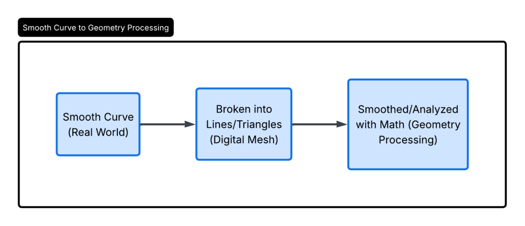
Geometry is a branch of Mathematics that studies properties of space such as shape, size, distance, and relative position of objects.

Geometry processing is a subfield of Computer Graphics (more generally, Computer Science and Engineering) and Applied Mathematics that develops algorithms to analyze, reconstruct, edit, and simulate 3D shapes

Essentially, geometry processing is the field that sits between “a shape exists” and “a computer can do something useful with that shape.”

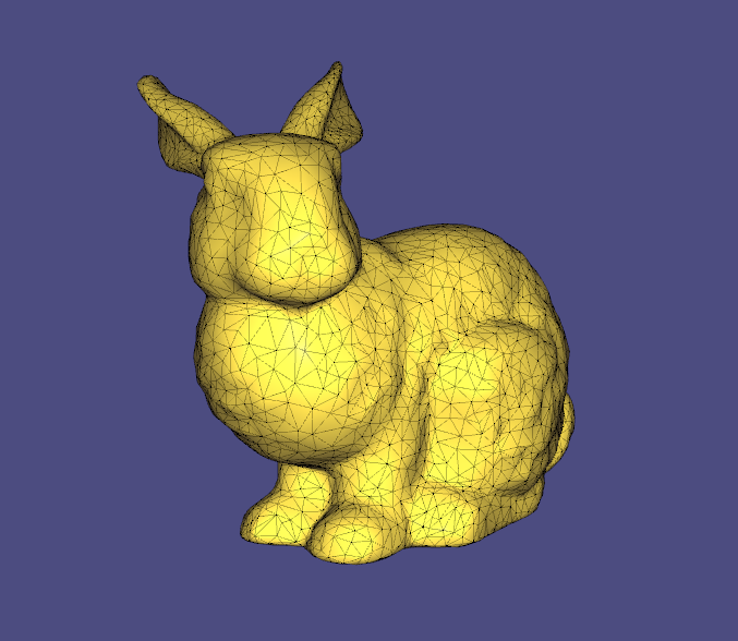
Think of a 3D mesh as a mountain scanned by a drone, a character in a game, a protein structure, or your own face captured by a phone camera. To a computer, that’s just a giant list of triangles: vertices, edges, faces. No inherent sense of “smooth,” “curved,” “similar to this other shape,” or “this is the front.”

The Stanford Bunny (source: https://en.wikipedia.org/wiki/File:Mesh_bunny.png)

Geometry processing is the toolkit that puts that sense back in. It asks questions like:

  • How curved is this surface, at this specific point, and how do we even define “curved” without calculus breaking on a sharp mesh edge?
  • If I deform this shape, what stays invariant?
  • Can I describe this shape as “a point in a space of shapes” so that “similar shapes” means “nearby points”?

and so on.

Process Overview

At first glance, geometry processing may seem like just another area of computer graphics. In reality, it draws ideas from differential geometry, linear algebra, numerical analysis, optimization, and computer science. Throughout SGI Tutorials Week, Fellows explored this interdisciplinary field from several complementary perspectives, each highlighting a different way of thinking about the same geometric object.

Now, why is this perspective important?

Earlier during the Tutorials Week, we were introduced to the field of Geometry and Geometry Processing from four different perspectives.

To the

  1. Layman – A figurative shape may hold some value but not necessarily insight.
  2. Mathematician – The same shape gives rise to a plethora of questions followed by a paramount of insight. The Mathematician defines the shape as a smooth manifold, which is a surface that locally looks like flat Euclidean space, allowing us to measure lengths, angles, and areas on it. The main challenge lies in approximating smooth geometry using triangles. Gaussian curvature K is defined from the shape operator (equivalently, the product of the principal curvatures). A remarkable result, the Gauss–Bonnet theorem, connects the total curvature of a surface to its topology (for a closed surface):
    MKdA=2πχ(M)\int_M K \, dA = 2\pi \chi(M)where χ\chi is the Euler characteristic (a single number that measures the global topology and “hole structure” of a 3D object or 2D surface).

  3. Programmer – While the Mathematician views the pristine manifold with rigor and perfection, the Programmer’s world demands that it be represented as a discrete mesh. This means the “manifold” from the mathematician’s world has to be discretized, and every discrete operator is an approximation whose convergence to the smooth operator must be justified as the mesh is refined. One common discrete analogue of Gaussian curvature is the angle defect at a vertex v:
    K(v)=2πiθiK(v) = 2\pi – \sum_{i} \theta_i
    where θi\theta_i​ are the interior angles of the triangles meeting at v.

    Flat vertex (angles sum to 2π2\pi) means zero curvature. A cone-like vertex results in nonzero curvature. Behind the scenes, it’s all discrete mathematics bonding with mathematical theorems, which gives rise to some wonders to be discussed in the Artist’s section.
  4. Artist – The Artist’s lens allows them to spot any phenomenon, in the absence of rigorous Mathematics or heavy computation, to give insights that are meaningful regardless of your background. The Artist appreciates what the scientifically grounded eye misses. To illustrate this perspective, I rendered several visualizations of the Stanford Bunny using Open3D.

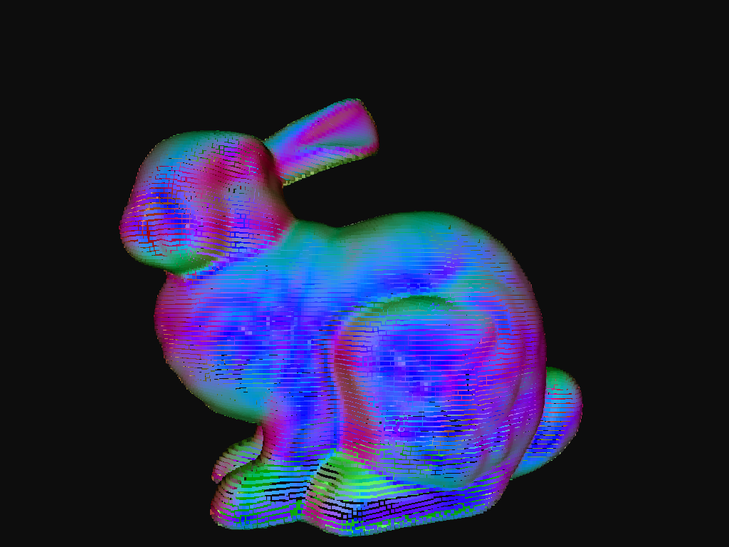
Surface normals: vectors indicating which direction the surfaces of the standard Stanford Bunny 3D model are facing, used for accurate lighting and 3D processing.
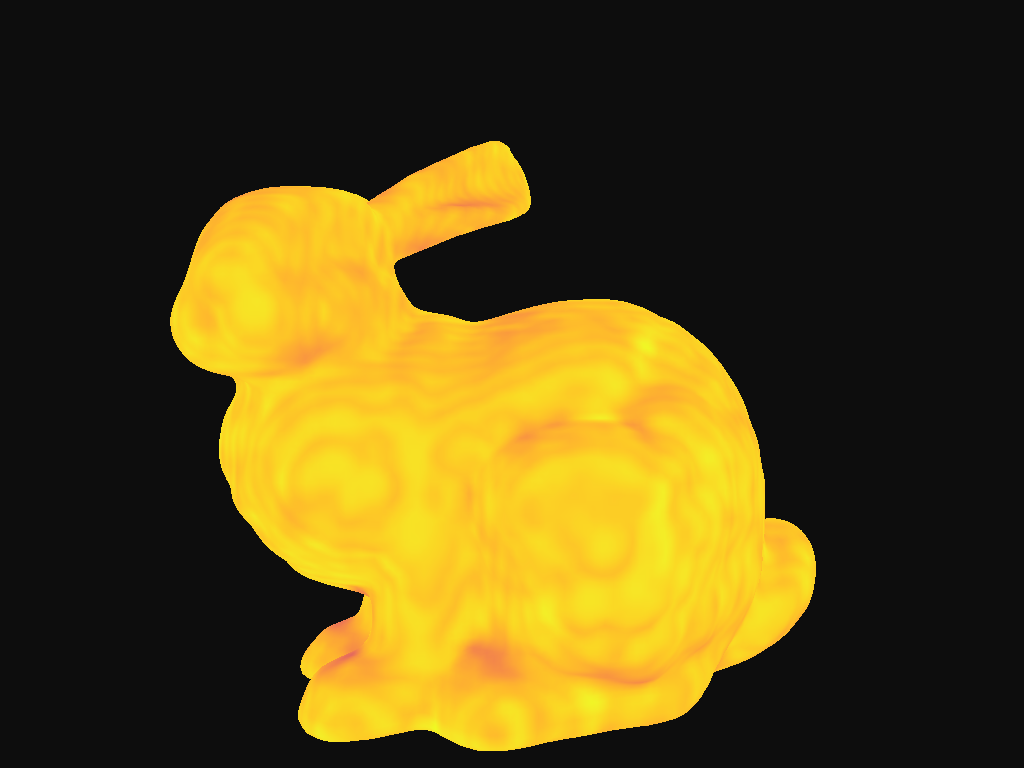
Stanford Bunny with Poisson Density
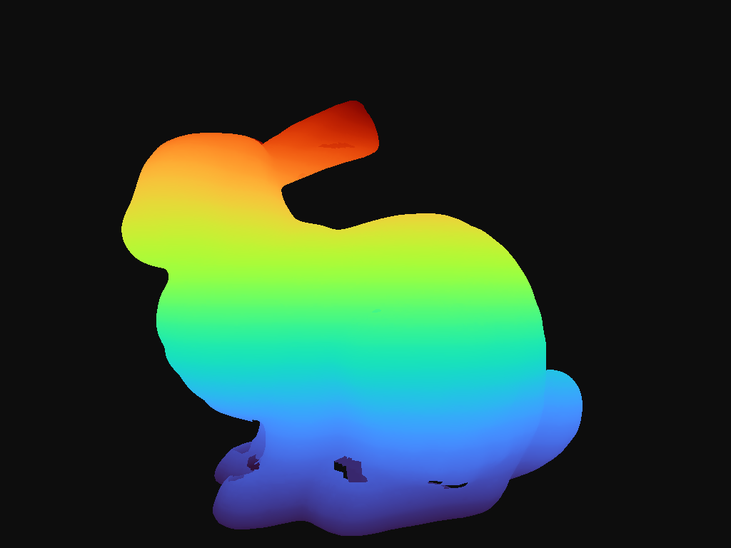
Elevation map
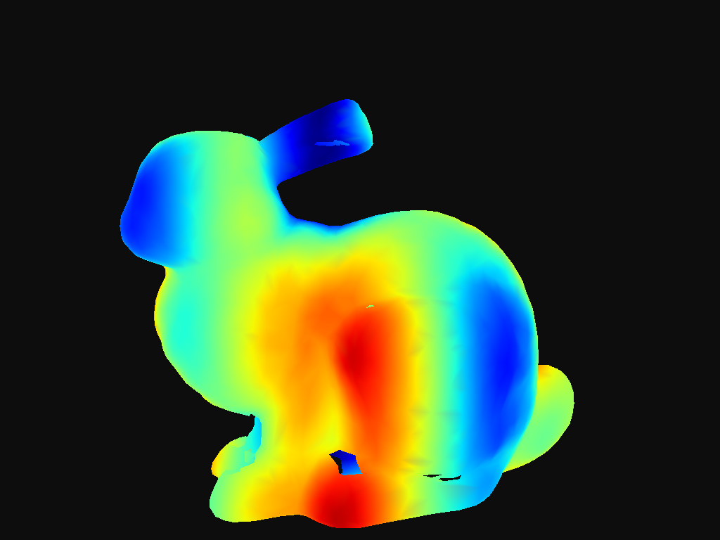
Wireframe curvature
Voxelized bunny view

And in a nutshell, that’s the beauty of this field. It is visually stunning, mathematically rigorous, and computationally elegant. And above everything, fascinating enough to sustain a research area for nearly half a century now.

Thank you to everyone at SGI for this wonderful initiative and for facilitating my research experience this summer.

Categories
Research

Navigating the Galaxy: RRT-Connect, C-Space, and Narrow Passages

Have you ever tried moving a sofa through a narrow staircase? Every twist, turn, and pivot matters, and one wrong angle means you’re stuck. In robotics and computational geometry, this is famously known as the “Piano Mover’s Problem.”

But what if the “piano” is a highly intricate, symmetrically interlocked mathematical sculpture?

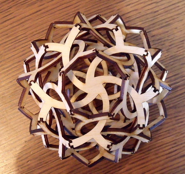
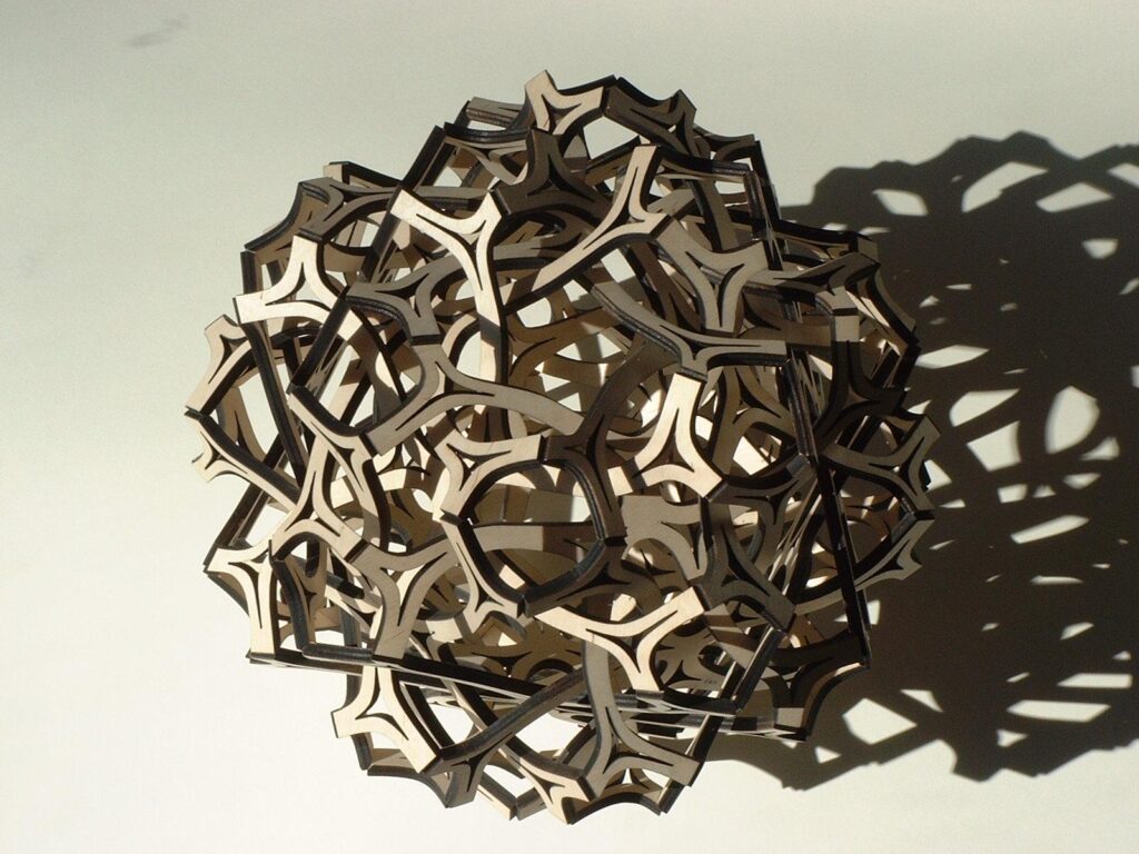
For my project, I decided to tackle the challenge of computationally disassembling the beautiful, mind-bending geometric sculptures designed by George Hart.

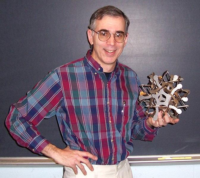
George Hart with a physical sculpture

To do this, I built a motion planning pipeline using the Open Motion Planning Library (OMPL) to find collision-free paths, Polyscope to visualize the 3D physical world, and Matplotlib to peek into the “brain” of the algorithm by plotting the 2D Configuration Space (C-Space).

Let’s dive into how we can use geometry to escape the cage, navigate the galaxy, and eventually… get completely snarled.

The Setup: Workspace vs. Configuration Space

To disassemble these symmetric sculptures, all identical pieces must move away from the center simultaneously. To simplify our problem, we define our state by a translation displacement “d” and a local rotation. While our algorithm supports rotation in “x”, “y”, and “z”, we found that moving outward with respect to the origin and rotating around the Z-axis is often the key to unlocking these puzzles.

This gives us two very different ways to look at the same problem:

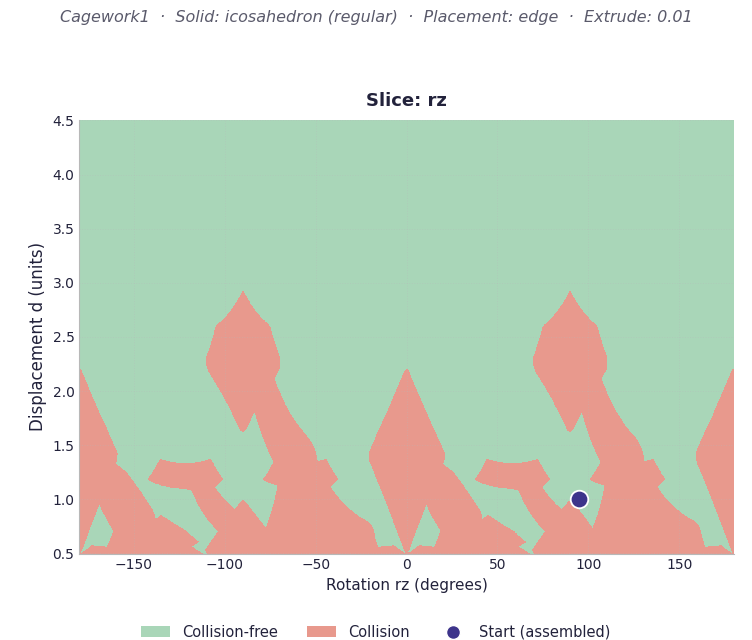
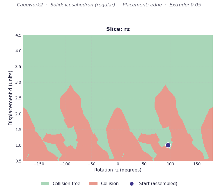
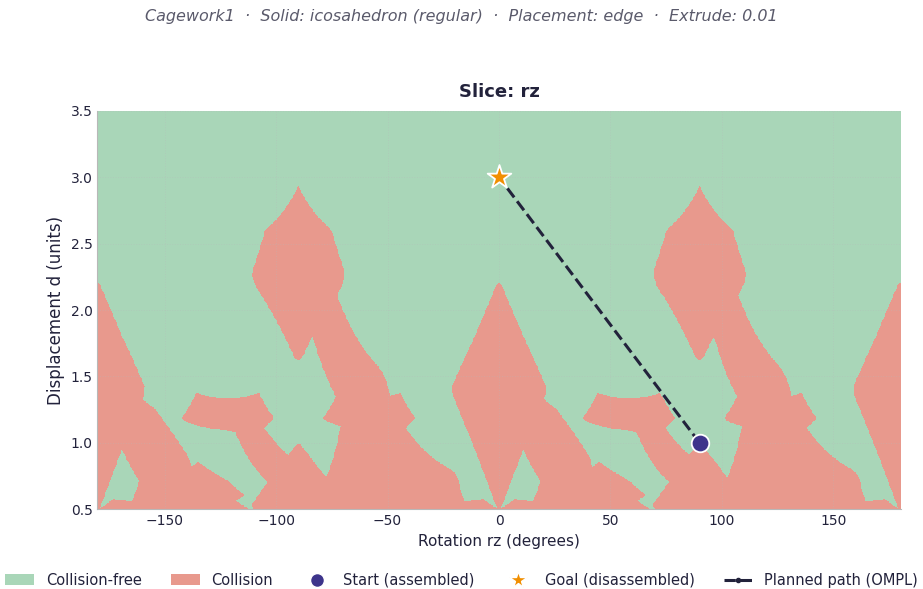
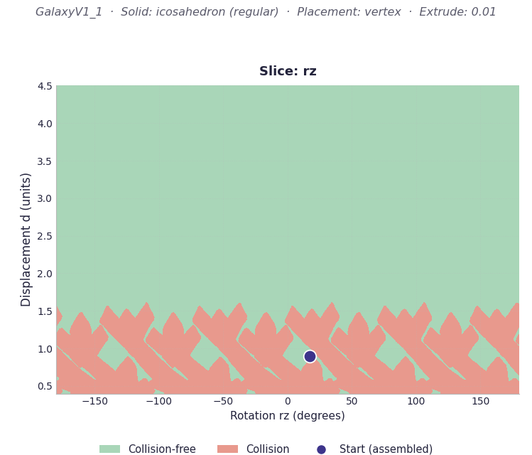
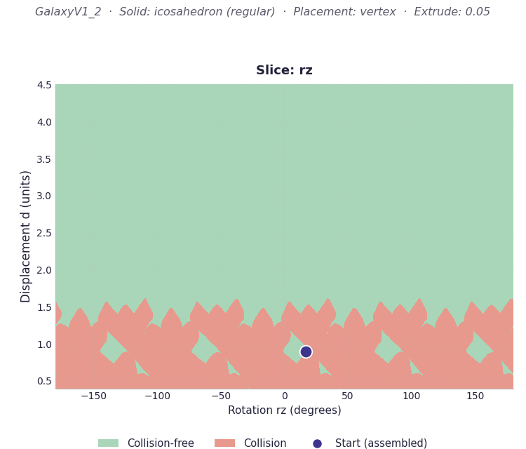
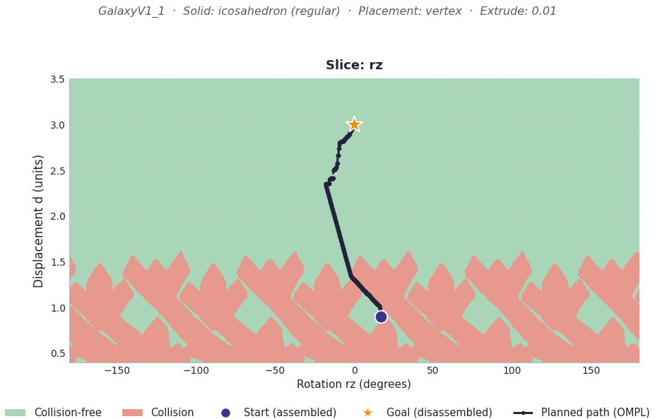
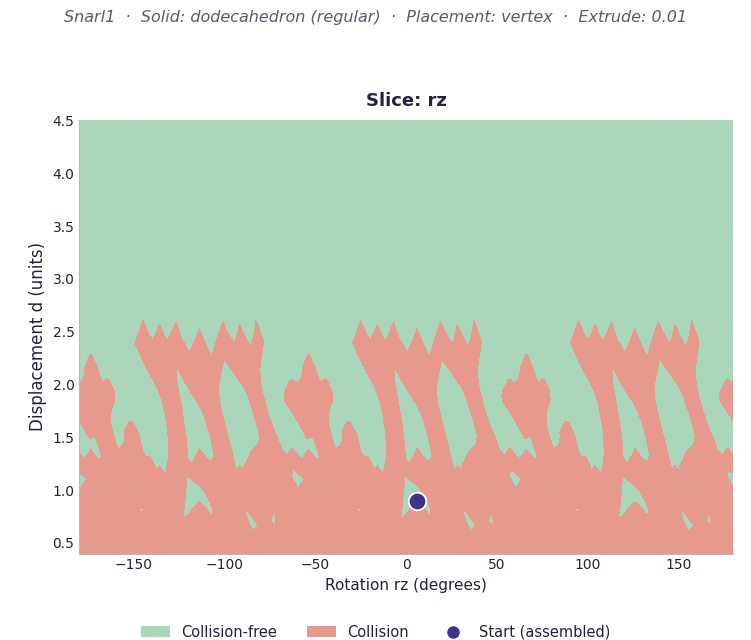
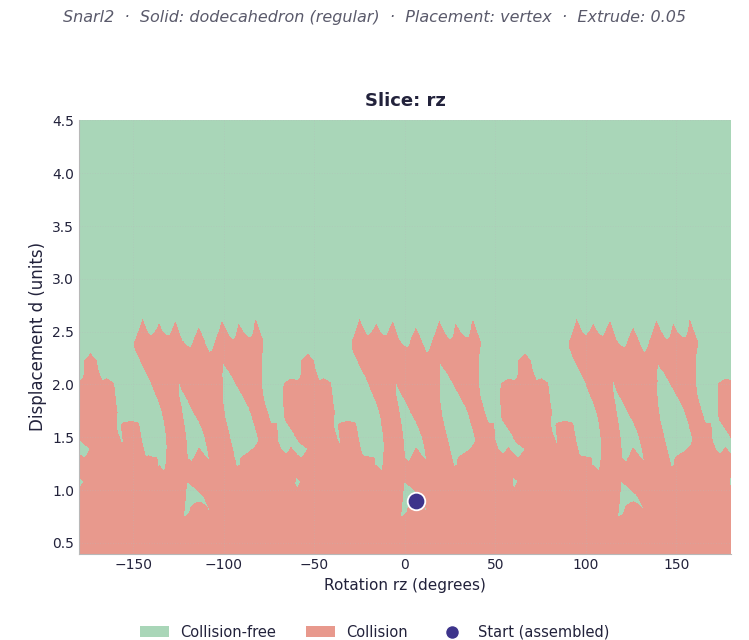
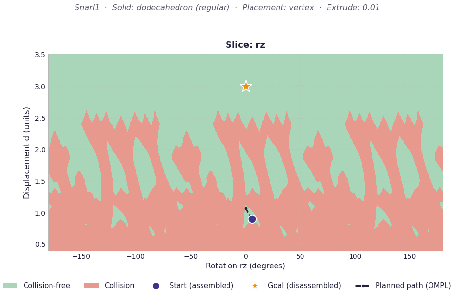
The C-Space (Matplotlib): The Configuration Space is a theoretical space where the entire sculpture is represented as a single point. I used Matplotlib to take 2D slices of this space (Displacement “d” vs. Rotation in Z). We evaluate thousands of states using the FCL (Flexible Collision Library). If a state has overlapping meshes, we color it red (Collision). If it’s safe, we color it green (Free Space).

The Workspace (Polyscope): This is the 3D physical space where the meshes actually exist and move. It’s what we see with our eyes.

The Algorithm: Growing Trees with OMPL

To find a valid path from the assembled state (Start) to the fully separated state (Goal), I used RRT-Connect from OMPL.

Imagine two vines growing blindly—one from the Start state and one from the Goal state. They branch out randomly into the free space of our C-Space, hoping to eventually touch and connect.

RRT-Connect is incredibly fast in wide-open spaces. However, it has a famous Achilles’ heel: The Narrow Passage Problem. If the only way to solve a puzzle is through a tiny, precise series of movements, the random vines have a very low probability of growing exactly into that microscopic corridor.

To test this, I ran the planner on three different George Hart sculptures. Here is what happened.

Experiment 1: Cagework (The Walk in the Park)

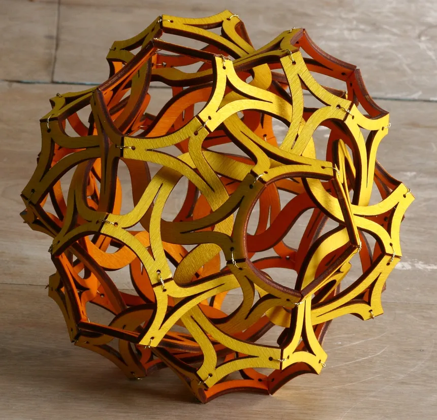
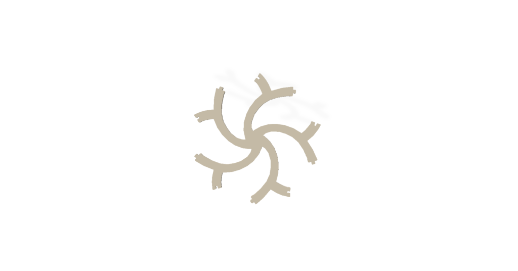
We started with Cagework. In the physical world, it looks like a complex cage of intersecting edges. But what does the algorithm see?

Because the C-Space has wide, forgiving green areas, our RRT-Connect algorithm has no trouble finding a path. Any random sample is likely to fall in a valid state.

The result in the workspace is a smooth, immediate disassembly.

Experiment 2: Galaxy (The Narrow Passage)

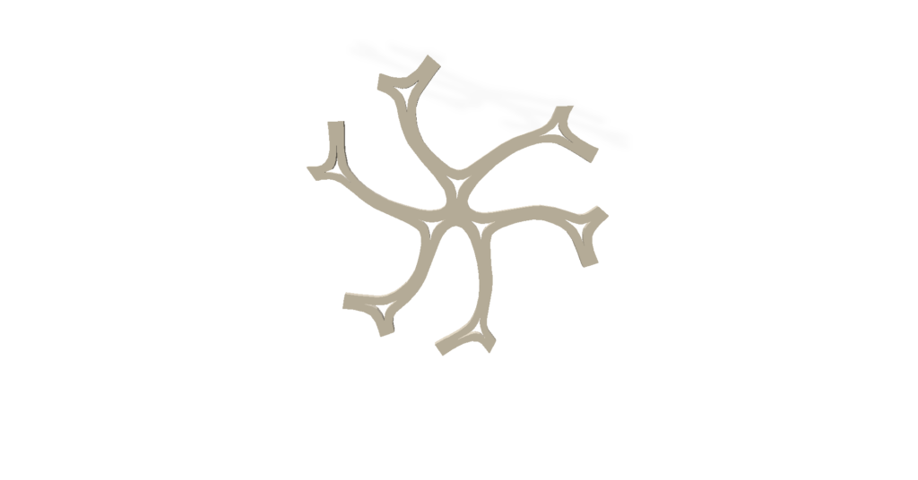
Next, we tried Galaxy. This is where things got interesting. The pieces are much more tightly packed, requiring a very specific twisting motion to separate.

This is a classic narrow passage. OMPL’s RRT-Connect had to work much harder here. The algorithm threw thousands of random branches, most of them hitting the red “collision” walls, until one lucky branch managed to thread the needle through the bottleneck.

When we animate the OMPL path in Polyscope, you can see exactly why this was so hard: the pieces barely scrape past each other, requiring a perfectly timed Z-rotation paired with the outward displacement.

Experiment 3: Snarl (The Impossible Snag)

Finally, we tested Snarl. As the name implies, this sculpture is a geometric knot. I set up the planner, hit run, and… nothing. The planner timed out. Instead of staring at a blank screen, we can use our Matplotlib C-Space plots to diagnose why it failed.

The 2D C-Space slice tells the whole story. The green space is completely disconnected, or the required passage is so microscopically narrow that it falls below our collision_tolerance (0.0001) and state_validity_resolution. The vines of our RRT-Connect were trapped in a cage of collisions, unable to reach the goal.

While a pure symmetrical displacement + rotation couldn’t solve Snarl, this “failure” is actually a success in visualization. It proves that the topology of the sculpture inherently locks itself in place under these symmetric constraints!

Conclusion & Future Work

Working on this project was a fantastic journey into how robots “think” about space. What looks like a physical interlocking puzzle to us is just a maze of high-dimensional obstacles to an algorithm.

By bridging OMPL, Polyscope, and Matplotlib, I learned that:

  1. Visualization is debugging: I wouldn’t have understood why Snarl failed without plotting the C-Space.
  2. Topology dictates performance: An algorithm is only as fast as the width of its narrowest passage.

In the future, it would be fascinating to expand the Matplotlib visualization to 3D slices (adding Rx or Ry into the mix) to see if Snarl has a hidden escape route in higher dimensions, or to implement path smoothing to make the Galaxy disassembly look less erratic.

A huge thank you to the SGI mentors and the amazing community for this experience!

Categories
Research

Surface Log Maps

by Anja Milutinovic and Shannon Cudworth

Geodesics and geodesic distance

Suppose we have a curved surface M⊂3\mathbb{R}^3. If we want to measure distances or move from one point to another, Euclidean straight lines are no longer appropriate because they leave the surface. So we generalise the notion of a “straight line”, by seeking the straightest possible path that remains on the surface. This is called a geodesic.

More formally, a geodesic is a curve that locally minimizes the length L of the curve:

L(γ)=01γ(t)dt,where γ(t)Tγ(t)M.L(\gamma)=\int_0^1 \|\gamma'(t)\|\,dt,\quad \text{where }\gamma'(t)\in T_{\gamma(t)}M.

The geodesic distance between two points p, q M is:

dM(p,q)=infγ:[0,1]M,γ(0)=p,γ(1)=qL(γ)d_M(p,q)=\inf_{\gamma:[0,1]\to M,\,\gamma(0)=p,\,\gamma(1)=q}L(\gamma)

Exponential and logarithmics maps

Given a point pMp\in M and a tangent vector vTpMv\in T_pM, there exists a unique geodesic γ\gamma such that γ(0)=p\gamma(0)=p and γ(0)=v\gamma'(0)=v. Exponential map Expp:TpMM\operatorname{Exp}_p:T_pM\rightarrow M is a map that for every vTpMv\in T_pM gives the endpoint of the geodesic starting at p with the direction vv and length v\|v\|

Then, the logarithmic map is the inverse of the exponential map,  Logp:MTpM\operatorname{Log}_p:M\rightarrow T_pM, whenever the exponential map is invertible. Logarithmic map for any given point qMq\in M is a tangent vector that gives the initial direction of a geodesic starting at p and ending at q.

Combining the logarithmic map with the frame ϕp:TpM2\phi_p:T_pM\rightarrow\mathbb{R}^2, we get 

z=ϕpLogpz=\phi_p\circ\operatorname{Log}_p, that maps any point q on a surface into 2\mathbb{R}^2.

Local parameterization of the Stanford Bunny using a logarithmic map centered at a selected point.

Levi Civita connections

Given two neighboring vertices v1,v2v_1, v_2 on a discrete triangle mesh, we can define corresponding tangent vectors t1,t2,t_1, t_2, such that t1t_1and t2t_2 belong to the tangent planes at v1v_1 and v2,v_2,respectively. Since t1, t2t_1,\ t_2 lie on different tangent planes, we cannot meaningfully compare them. Our goal is to define a parallel transport, which moves one tangent vector to another tangent plane at an adjacent vertex, while minimizing rotation, known as the Levi Civita connection.

To implement the Levi Civita connection, we are given a dictionary containing all vertices with a shared edge, and the normal vector defined at every vertex viv_i. By looping over all shared edges i,ji,j, we take neighboring vertices vi,vjv_i, v_j and we index and define the normal vectors corresponding with the vertices, labeled n1n_1 and n2n_2, respectively.  We then use the normals to calculate the Rodrigues Rotation, or the rotation of a vector by a specific angle around a fixed axis. The formula to determine this rotation matrix is given by:

R=I+vx+vx2×1cs2R = I + v_x + v_x^2 \times \frac{1-c}{s^2}

where v=n1×n2, c=n1n2, s=||v||, 𝐯×=[0v2v1v20v0v1v00]v = n1 \times n2,\ c = n1 \cdot n2, \ s = ||v||, \ \mathbf{v}_{\times}=\left[\begin{array}{ccc}0&-v_2&v_1\\v_2&0&-v_0\\-v_1&v_0&0\end{array}\right]

Then R approximates Levi Civita connection between adjacent tangent planes.

Connection Laplacian

After constructing the Levi Civita connection, we want to compare the tangent vectors at neighboring vertices, which is accomplished through the Connection Laplacian. As before, we loop over all vertices i,j with shared edges, and first define the cotangent weights, which are given by:

wij=12(cotαij+cotβij)w_{ij} = \frac{1}{2}(cot\alpha_{ij} + cot\beta_{ij})

where αij\alpha_{ij} and βij\beta_{ij} are the two angles opposite the edge (i, j). Now we can define the Connection Laplacian matrix, defined as:

Lij={(kN(i)wik)I,amp;i=j,wijRji,amp;(i,j) is an edge,0,amp;otherwise. L_{ij}= \begin{cases} \left(\displaystyle\sum_{k\in N(i)} w_{ik}\right)I, & i=j, \\[1.2ex] -w_{ij}R_{ji}, & (i,j)\text{ is an edge}, \\[0.8ex] 0, & \text{otherwise}. \end{cases}

where wijw_{ij} is the cotangent weight between vertex i and vertex j, RijR_{ij} is the Levi Civita connection between vertex i and vertex j, and N(i)N(i) is the set of adjacent vertices to vertex i. Once the Connection Laplacian is defined, we can now measure how tangent vector fields change across vertices and our mesh.

Heat Diffusion & Vector Heat Method

With the Levi Civita connection and the Connection Laplacian, we can now define the Vector Heat Method (VHM), which approximates parallel transports between arbitrary vertices on our surface.

Given a mass matrix M, a connection laplacian L, an initial vector field V, and a small time step h, we can solve the vector heat equation:

(M+hL)X=V(M + hL)X = V

where X is a vector field that approximates the parallel transport of V along the minimal geodesics.

We now introduce a set of user-selected seed vertices S = { s1, ... ,sks_1,\ … \ , s_k } ⊂V. Via the VHM, we can approximate the parallel transport between any arbitrary seed vertices. Our goal is to extend this to the Affine Heat Method, which will use the VHM estimations of parallel transport between seed frames to optimize a set of tangent frames, allowing adjacent logarithmic maps to be more effectively blended.

Seed graph with optimal frames & UV offset

A single logarithmic map only provides a low-distortion parameterization around one point on the surface. To cover the entire mesh, we choose a small set of seed verticesS={s1,,sk}V,S=\{s_1,\ldots,s_k\}\subseteq V,and compute one logarithmic map around each seed. Each seed defines its own local coordinate system describing the nearby geometry.

Since these maps are computed independently, their coordinate systems are arbitrary. Even if two neighboring maps describe the same part of the surface, one may be rotated relative to the other. Before we try to combine the maps, their orientations must be made consistent.

We therefore associate each seed with a local frame tsTsMt_s \in T_sM. Specifically, we define a linear map Ψs:TsMR2\Psi_s : T_sM \rightarrow \mathbb{R}^2 that maps the local frame to the horizontal axis of the plane.

However, the maps may still be translated.o fix this, we assign each seed a UV offset wsR2w_s\in\mathbb{R}^2. Neighboring logarithmic maps should predict the same relative displacement, leading to the consistency condition:

wsws+Ψs(logs(s)).w_{s’} \approx w_s + \Psi_s\!\left(\log_s(s’)\right).

he UV offsets are then computed by minimizing the disagreement between neighboring seeds.

Blending seed’s log maps

The final step was to combine the local parameterizations into a single global UV map. This involves deciding which local maps influence each part of the surface and how they should be combined. One way to this is to partition the surface into Voronoi cells, where each vertex is assigned to its nearest seed according to geodesic distance and inherits that seed’s local parameterization. While this approach is simple and efficient, it creates visible seams at the boundaries between neighboring cells.

Global UV parameterization of the Stanford Bunny using a Voronoi partition of local logarithmic maps.

Categories
Tutorials

From Discrete Points to Smooth Manifolds: The Elegant Architecture of Geometry Processing

To a layperson, geometry is simply the study of interesting shapes, and geometry processing is the software pipeline that acquires, manipulates, and outputs them. But to researchers, mathematicians, and programmers in computational geometry, a surface represents something far deeper. It is a continuous topological space that is locally homeomorphic to a Euclidean plane. The defining challenge of geometry processing is discretized representation. How do we preserve the continuous, elegant properties of smooth differential geometry within the rigid, discrete confines of computer memory?

Discrete Topology: The Piecewise Approximation of Manifolds

In computer graphics and geometric modeling, we mathematically transition from smooth 1D polylines to 2D surfaces by utilizing triangle meshes. These meshes are piecewise-linear approximations of continuous surfaces. Under the hood, this elegant approximation relies on a surprisingly simple graph-based data structure: the vertex-list-face-list representation.

Rather than storing redundant spatial coordinates for every single polygon, the geometry is split into two clean matrices:

The Vertex List

An n x 3 matrix storing the precise spatial coordinates (xi, yi, zi) of every triangle corner in 3D space:

V = {x1 y1 z1

x2 y2 z2

Xn yn zn }

The Face List

An m x 3 matrix storing the topological connectivity. Each row contains three integer indices that reference the vertex list, defining exactly which three vertices form a triangle face:

F = ( f1,1 f1,2 f1,3

f2,1 f2,2 f2,3

fm,1 fm,2 fm,3 )

By decoupling the spatial geometry (the vertex coordinates) from the topological connectivity (the face indices), a triangle mesh is fundamentally transformed into a graph. This structure is incredibly robust. It allows scientists to build closed 3D topologies, such as a simple tetrahedron, or represent incredibly complex, high-resolution models like the classic Stanford Bunny or Blender’s Suzanne monkey head. In fact, standard exchange formats like .obj store this exact coordinate and index pairing directly.

Defining Functions and Interpreting Fields

Once a surface is represented as a mesh, the next frontier in geometry processing is defining functions over these domains. Mathematically, a function f maps elements from a geometric domain to a codomain, such as mapping points on a 2D surface to real-world scalar values:

f:R² — R, f(x,y) = x² + y²

In practical applications, these functions represent physical properties like temperature distribution, deformation fields, or surface texture coordinates. However, visualizing and analyzing these continuous mathematical fields on a discretized computer screen introduces another layer of complexity: shading and perspective. A critical part of geometry processing is knowing how to interpret these plots, as the choice between flat rendering, smooth Gouraud/Phong shading, and shadow mapping drastically alters our perception of the underlying geometric curvature.

Hands-On Exploration

For researchers looking to prototype algorithms, compute discrete differential operators, or visualize complex functions on manifolds, modern Python ecosystems make these tools highly accessible. Using the gpytoolbox library for geometry operations and polyscope for rich, interactive 3D visualization, you can implement and observe these geometric principles firsthand.

Categories
Tutorials

Connecting the Dots: How Computers Map Geometry Using Polylines

To represent visual shapes and curves digitally, computer systems must translate geometry into structured, machine-readable data. While simply storing a finite set of coordinate points is highly memory-efficient, this method lacks the connectivity information required to define a cohesive shape. By pairing these coordinate points with explicit connectivity instructions and applying linear interpolation, which mathematically draws straight lines between designated point pairs, computers construct a “polyline” that successfully bridges the gap between raw spatial data and continuous geometric forms.

This polyline framework serves as a cornerstone of computational geometry due to its remarkable efficiency and versatility. By breaking complex curves down into simple, straight line segments, polylines are exceptionally easy for graphics cards to store and render rapidly on screen. Furthermore, this linear structure simplifies complex spatial calculations, making it highly efficient for software to query spatial relationships or calculate geometric intersections, such as determining where a path crosses a boundary.
Categories
Administrative

Behind the SGI 2026 Mug

Hello, my name is Oras, and I am the main designer behind the SGI 2026 mug :). I wanted to write a bit about the design process, and to also share some design tidbits that may not be so obvious from the outside.

Flat form of the final design, to be wrapped around a mug

One very nice thing about SGI that I have not seen talked about much: because the first iteration of SGI occurred in 2021, the last digit of the year tells us which iteration we are in! (At least, until 2029.) This year, 2026, corresponds to the 6th cohort, so I set out to use the number 6 as often as possible in my design.

SGI as a program is all about geometry. Now, what kind of geometric patterns we can use that look pretty and can incorporate the number 6? The first thing my mind went to was…

The Fractals

Fractals are self-similar patterns, usually generated from a very concise set of predefined rules. Apart from being very mathematical, I also find them incredibly satisfying to look at. Most readers will likely be familiar with the Sierpinski triangle seen in the fractals sequence. A triangle is scaled down, copied three times, and put at the corners of the original triangle. Then you repeat the process.

Sierpinski triangle

But what about the other ones? Turned out, the concept of Sierpinski polygons does actually generalize to any n-gon, and that is what all these shapes are!

So the choice was obvious: I wanted to feature the Sierpinski hexagon in my design. And what does it look like? Well, not as interesting as its triangle counterpart, as it turned out.

Basic Sierpinski hexagon

It’s not horrible by any means, but I was hoping to use this as the attention grabber, and this variation had more negative space than I would’ve liked. It also looked too regular for my taste. What I like about fractals is the controlled chaos, how it can look locally chaotic yet attains a striking symmetry as a whole.

Turned out, there was a way to mitigate this: a Sierpinski polygon depends on the scaling factor rr. In order for the iterated shape to fit together without overlapping, a specific rr value has to be used, depending on the number of sides. For hexagons, r=13r=\frac{1}{3} is the “correct” ratio.

First iteration of the Sierpinski hexagon visualizing the scaling factor

What happens when we vary rr? We get some pretty interesting results!

Sierpinski hexagon with the scaling factor (r) varying between 1/2 and 1/3

We can also do the same for pentagons, whose “correct” scaling factor is r=11+ϕ12.618r=\frac{1}{1+\phi} \approx \frac{1}{2.618}, where ϕ\phi is the golden ratio

Sierpinski pentagons with scaling factor (r) varying between 1/2 and 1/2.618

In the end, I just chose an rr value that looked good. For the hexagon, that turned out to be r=11+2r=\frac{1}{1+\sqrt{2}}. I did not realize this at the time, but this was a fairly special value: it was the value that made the corners of the hexagons “touch” at the third iteration. The result: the gaps between hexagons form perfect six-sided stars with sharp points!

(I didn’t realize this at the time, so the pentagon just used a somewhat random value of r12.273r \approx \frac{1}{2.273}. Question for the readers: what would be an equivalent rr for a pentagon?)

Bonus: the six iterations of the Sierpinski hexagon and pentagon

Progression of Sierpinski hexagon from iteration 1 to 6
Progression of Sierpinski pentagon from iteration 1 to 6

And yes, I use 6 iterations for all of the fractals, so there’s another hidden number 6 for you ;).

What About the Other Ones?

I wanted to have a sequence of 6 fractals, symbolizing the iterations of SGI itself, which would increase in sophistication and complexity over time. The Sierpinski triangle was simple enough, but how would I make Sierpinski 2-gon and 1-gon? This took some interpretations

  • For the 1-gon, I decided to treat it as a point, which has no size. So a Sierpinski-type iteration would just product a point. I visualized this with an empty circle, since you technically can’t draw an infinitesimal point on a 2D canvas.
  • I interpreted 2-gon as a line, with the two sides overlapping. Since it also has no area, a Sierpinski 2-gon would also be just a line. To make this more interesting, I decided to create a binary tree instead, which is create from a set of self-similar “I” shapes.
  • Sierpinski square was replaced with a QR code leading to the SGI website ;).
Iterated figure “I” (or maybe short H?) used to represent Sierpinski “2-gon”

Honorable Mentions

I considered a few other fractals to include in the design as well, but ended up going for a simpler design, partially due to time constraint.

Koch’s Snowflake

4 iterations of Koch’s snowflake

Very iconic, and a natural fit for the number 6. I decided against using it in the end because it was a little too well known, and I wanted a more unique look for our mug.

Dragon Curve

10th iteration of the Dragon curve, illustrating the limit shape

Arguably my favorite fractal of all time, especially for its connection to paper folding. Unfortunately, I couldn’t quite figure out how to incorporate it into the design. And there is also a similar issue of negative space: the interesting parts are at the outline, but the interior is plain.

Levy Dragon

Fancy SGI acronym made from a bunch of Levy Dragons

For a while, I really wanted the SGI acronym itself to be a fractal. I ended up playing around the the Levy Dragon, which I arranged into the letters. In the end, I decided it was much too ornate compared to the rest of the design, and did not use it.

Other Mug Designs

There were many other awesome mug designs proposed, most of which served as inspirations for my design!

Gokul S was the first person who proposed a design element in the group chat: a sequence of L-System-based trees. I basically stole the six-fractals-sequence-as-SGI-cohorts from him. I tried really hard to include these trees in my design as well, but unfortunately could not find a good place for them in time :(.

Similarly, Rahim Hossain proposed using levels of decimation of a Stanford Bunny, which I also copied wholesale into my design.

Kyle Loh created this awesome design. In his own words:

[The design] is a continuous-time dynamical system called the Thomas attractor (it is strange and chaotic, by the way).

Finally, Loiruck Godwin proposed a couple of designs, featuring a “grid of bunnies,” and a crystalline cliff that “captures the collaborative nature of SGI, where people of various background’s help each other and work together to climb a geometric mountain of knowledge.”

I would not have been able to push my design as far as I could without these inspirations, and I’m glad I get to at least showcase these designs here, as they deserve to be :).

Final Thoughts

Apparently, a blog post doesn’t feel complete without a concluding section like this, but I also don’t really have a conclusion to offer. So I will just include some tidbits about the design I couldn’t fit elsewhere.

  • The first iteration of the design incorporated a giant number 6. My logic was “if you look at this mug on your shelf from a distance, you’d be able to tell it’s the SGI 6 mug right away!” Turned out, everyone unanimously hated the giant 6 😂. Subsequent design iterations featured the year 2026 of a regular size.
The first iteration of the design with the universally hated giant number 6
  • One goal I had for the design was it MUST look good wrapped around a mug. Blender was very useful for visualizing this. I downloaded a 3D mesh of a mug from Sketchfab, and learned to manually unwrap the UV for the first time, which was fun :).
3D visualization was how I realized the borders on my original design would have introduced a very harsh edge, and were thus removed in subsequent designs
Categories
Administrative

Welcome to SGI 2026!

Welcome to the official blog of the Summer Geometry Initiative (SGI) 2026, taking place July 6-August 14! I’m Justin Solomon, director of SGI 2026 and PI of the MIT Geometric Data Processing Group.

First launched in 2021, SGI is a completely online program engaging a paid cohort of undergraduate and early master’s students in six weeks of training and research experiences related to applied geometry and geometry processing. SGI Fellows come from all over the globe and represent a wide variety of educational institutions, life/career paths, and fields of interest.

SGI aims to accomplish the following objectives:

  • spark collaboration among students and researchers in geometry processing,
  • launch inter-university research projects in geometry processing involving team members across broad levels of seniority (undergraduate, graduate, faculty, industrial researcher),
  • introduce students to geometry processing research and development, and
  • expand the “pipeline” of students entering geometry processing research.

SGI aims to address a number of challenges and inequities in geometry processing. Not all universities host faculty whose work touches on this emerging field, reducing the cohort of students exposed to this discipline during their undergraduate careers. By giving a broad set of students access to geometry processing research experiences, over the longer term we hope to affect the composition and size of the geometry processing community.

SGI is supported by a worldwide network of volunteers, including faculty, graduate students, and research scientists in geometry and related disciplines. This team supports the SGI Fellows through mentorship, instruction, panel discussions, and several other means.

SGI 2026 is due to start in a few days! Each SGI Fellow will be mailed a box of swag from our many sponsors, a certificate, and a custom-made coffee mug designed by SGI 2026 Fellow Oras Phongpanangam and others.

We’ll kick off next week with tutorials in geometry processing led by Oded Stein (Technion), Silvia Sellán (Columbia University), Nicole Feng (Carnegie Mellon University), Dale Decatur/Richard Liu (University of Chicago), and Nick Sharp (NVIDIA). Then, in the remaining 5 weeks, our Fellows will have the opportunity to participate in multiple short-term (1-2 week) research projects, intended to kick off collaborations that last over the longer term. Check out last year’s SGI blog for examples of the kinds of projects they’ll be working on.

Revisit this blog as the summer progresses for updates on SGI 2026 and to read about the exciting ideas our Fellows are developing in geometry!