Categories
Tutorials

A Beginner’s Take On Geometry & Geometry Processing

Hello! My name is Nafisa Nawrin Labonno, and I am an undergraduate student at the University of Texas at Arlington, studying Physics and Computer Science. In this blog post, I will walk you all through my journey as an SGI 2026 Fellow.
To a beginner, everything feels exciting and overwhelming. But to a curious beginner, things feel challenging enough to channel their inquisitiveness into something meaningful. I would say this is my experience with my fellowship at SGI. From the tutorials week to my first week of mentored research here at SGI, I had an amazing time dipping my toe into the shallow waters of Geometry, which is eventually (and hopefully) taking a deep dive into wonderful research.

Geometry is a branch of Mathematics that studies properties of space such as shape, size, distance, and relative position of objects.

Geometry processing is a subfield of Computer Graphics (more generally, Computer Science and Engineering) and Applied Mathematics that develops algorithms to analyze, reconstruct, edit, and simulate 3D shapes

Essentially, geometry processing is the field that sits between “a shape exists” and “a computer can do something useful with that shape.”

Think of a 3D mesh as a mountain scanned by a drone, a character in a game, a protein structure, or your own face captured by a phone camera. To a computer, that’s just a giant list of triangles: vertices, edges, faces. No inherent sense of “smooth,” “curved,” “similar to this other shape,” or “this is the front.”
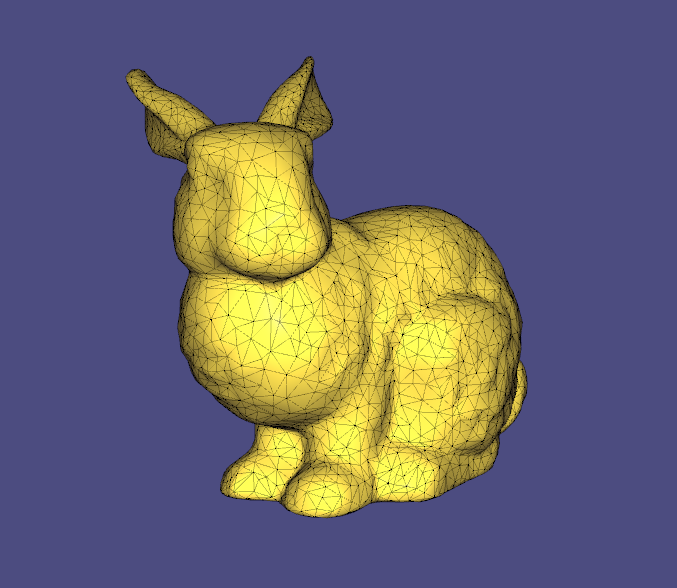
The Stanford Bunny (source: https://en.wikipedia.org/wiki/File:Mesh_bunny.png)

Geometry processing is the toolkit that puts that sense back in. It asks questions like:

  • How curved is this surface, at this specific point, and how do we even define “curved” without calculus breaking on a sharp mesh edge?
  • If I deform this shape, what stays invariant?
  • Can I describe this shape as “a point in a space of shapes” so that “similar shapes” means “nearby points”?

and so on.

Process Overview

At first glance, geometry processing may seem like just another area of computer graphics. In reality, it draws ideas from differential geometry, linear algebra, numerical analysis, optimization, and computer science. Throughout SGI Tutorials Week, Fellows explored this interdisciplinary field from several complementary perspectives, each highlighting a different way of thinking about the same geometric object.
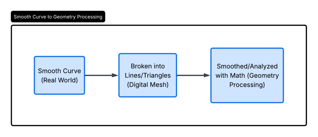
Now, why is this perspective important?

Earlier during the Tutorials Week, we were introduced to the field of Geometry and Geometry Processing from four different perspectives.

To the

  1. Layman – A figurative shape may hold some value but not necessarily insight.
  2. Mathematician – The same shape gives rise to a plethora of questions followed by a paramount of insight. The Mathematician defines the shape as a smooth manifold, which is a surface that locally looks like flat Euclidean space, allowing us to measure lengths, angles, and areas on it. The main challenge lies in approximating smooth geometry using triangles. Gaussian curvature K is defined from the shape operator (equivalently, the product of the principal curvatures). A remarkable result, the Gauss–Bonnet theorem, connects the total curvature of a surface to its topology (for a closed surface):
    MKdA=2πχ(M)\int_M K \, dA = 2\pi \chi(M)where χ\chi is the Euler characteristic (a single number that measures the global topology and “hole structure” of a 3D object or 2D surface).
  3. Programmer – While the Mathematician views the pristine manifold with rigor and perfection, the Programmer’s world demands that it be represented as a discrete mesh. This means the “manifold” from the mathematician’s world has to be discretized, and every discrete operator is an approximation whose convergence to the smooth operator must be justified as the mesh is refined. One common discrete analogue of Gaussian curvature is the angle defect at a vertex v:
    K(v)=2πiθiK(v) = 2\pi – \sum_{i} \theta_i
    where θi\theta_i​ are the interior angles of the triangles meeting at v.

    Flat vertex (angles sum to 2π2\pi) means zero curvature. A cone-like vertex results in nonzero curvature. Behind the scenes, it’s all discrete mathematics bonding with mathematical theorems, which gives rise to some wonders to be discussed in the Artist’s section.
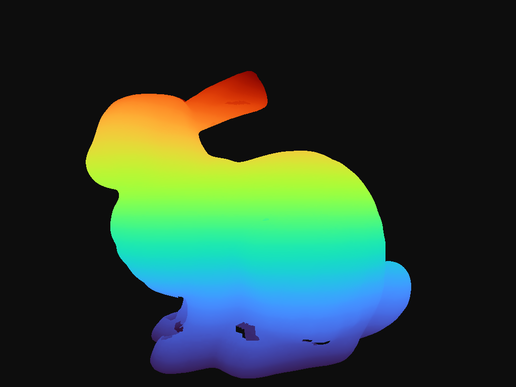
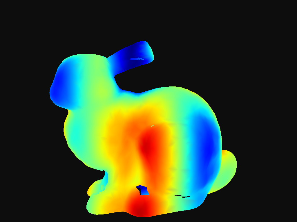
  4. Artist – The Artist’s lens allows them to spot any phenomenon, in the absence of rigorous Mathematics or heavy computation, to give insights that are meaningful regardless of your background. The Artist appreciates what the scientifically grounded eye misses. To illustrate this perspective, I rendered several visualizations of the Stanford Bunny using Open3D.
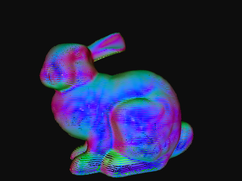
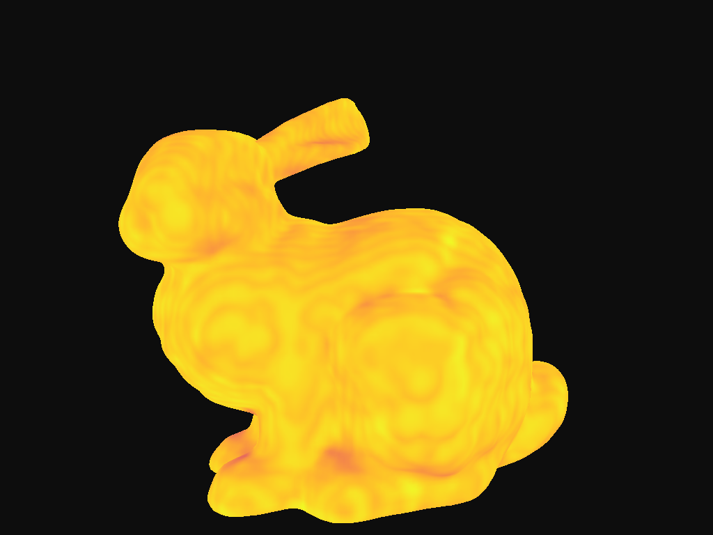
Surface normals: vectors indicating which direction the surfaces of the standard Stanford Bunny 3D model are facing, used for accurate lighting and 3D processing.
Stanford Bunny with Poisson Density
Elevation map
Wireframe curvature
Voxelized bunny view

And in a nutshell, that’s the beauty of this field. It is visually stunning, mathematically rigorous, and computationally elegant. And above everything, fascinating enough to sustain a research area for nearly half a century now.

Thank you to everyone at SGI for this wonderful initiative and for facilitating my research experience this summer.

Categories
Tutorials

From Discrete Points to Smooth Manifolds: The Elegant Architecture of Geometry Processing

To a layperson, geometry is simply the study of interesting shapes, and geometry processing is the software pipeline that acquires, manipulates, and outputs them. But to researchers, mathematicians, and programmers in computational geometry, a surface represents something far deeper. It is a continuous topological space that is locally homeomorphic to a Euclidean plane. The defining challenge of geometry processing is discretized representation. How do we preserve the continuous, elegant properties of smooth differential geometry within the rigid, discrete confines of computer memory?

Discrete Topology: The Piecewise Approximation of Manifolds

In computer graphics and geometric modeling, we mathematically transition from smooth 1D polylines to 2D surfaces by utilizing triangle meshes. These meshes are piecewise-linear approximations of continuous surfaces. Under the hood, this elegant approximation relies on a surprisingly simple graph-based data structure: the vertex-list-face-list representation.

Rather than storing redundant spatial coordinates for every single polygon, the geometry is split into two clean matrices:

The Vertex List

An n x 3 matrix storing the precise spatial coordinates (xi, yi, zi) of every triangle corner in 3D space:

V = {x1 y1 z1

x2 y2 z2

Xn yn zn }

The Face List

An m x 3 matrix storing the topological connectivity. Each row contains three integer indices that reference the vertex list, defining exactly which three vertices form a triangle face:

F = ( f1,1 f1,2 f1,3

f2,1 f2,2 f2,3

fm,1 fm,2 fm,3 )

By decoupling the spatial geometry (the vertex coordinates) from the topological connectivity (the face indices), a triangle mesh is fundamentally transformed into a graph. This structure is incredibly robust. It allows scientists to build closed 3D topologies, such as a simple tetrahedron, or represent incredibly complex, high-resolution models like the classic Stanford Bunny or Blender’s Suzanne monkey head. In fact, standard exchange formats like .obj store this exact coordinate and index pairing directly.

Defining Functions and Interpreting Fields

Once a surface is represented as a mesh, the next frontier in geometry processing is defining functions over these domains. Mathematically, a function f maps elements from a geometric domain to a codomain, such as mapping points on a 2D surface to real-world scalar values:

f:R² — R, f(x,y) = x² + y²

In practical applications, these functions represent physical properties like temperature distribution, deformation fields, or surface texture coordinates. However, visualizing and analyzing these continuous mathematical fields on a discretized computer screen introduces another layer of complexity: shading and perspective. A critical part of geometry processing is knowing how to interpret these plots, as the choice between flat rendering, smooth Gouraud/Phong shading, and shadow mapping drastically alters our perception of the underlying geometric curvature.

Hands-On Exploration

For researchers looking to prototype algorithms, compute discrete differential operators, or visualize complex functions on manifolds, modern Python ecosystems make these tools highly accessible. Using the gpytoolbox library for geometry operations and polyscope for rich, interactive 3D visualization, you can implement and observe these geometric principles firsthand.

Categories
Tutorials

Connecting the Dots: How Computers Map Geometry Using Polylines

To represent visual shapes and curves digitally, computer systems must translate geometry into structured, machine-readable data. While simply storing a finite set of coordinate points is highly memory-efficient, this method lacks the connectivity information required to define a cohesive shape. By pairing these coordinate points with explicit connectivity instructions and applying linear interpolation, which mathematically draws straight lines between designated point pairs, computers construct a “polyline” that successfully bridges the gap between raw spatial data and continuous geometric forms.

This polyline framework serves as a cornerstone of computational geometry due to its remarkable efficiency and versatility. By breaking complex curves down into simple, straight line segments, polylines are exceptionally easy for graphics cards to store and render rapidly on screen. Furthermore, this linear structure simplifies complex spatial calculations, making it highly efficient for software to query spatial relationships or calculate geometric intersections, such as determining where a path crosses a boundary.