Categories
Research

Research and Production for Games

Visualizing and Evaluating Skin Weight Transfer

My goal for this project was to implement visualization methods that help artists gauge the accuracy of skin weight transfer methods, which takes the skin weights from an already rigged mesh, and assigns the correct weights to the target mesh. I compared two different weight transfer methods. First, Maya’s built-in copySkinWeights: which takes a vertex on the unrigged mesh, finds the closest point on the source mesh, and interpolates the weights at that point to determine the weights at the vertex. Next, a method developed by EpicGames, which copies the weights from the source mesh that have a high-confidence correspondence. For the remaining vertices, it computes the weights by interpolating from the transferred high-confidence weights.

To begin, I downloaded a character with an animation from Mixamo and imported it into Maya. In my first pass comparison, I unbound the shirt from the character, and then rebound it using Maya’s copySkinWeights and EpicGames’ Weight Inpaint method. Below is a playblast of each character. Notice that with the copySkinWeights there is a jagged concave area in the upper back region, while with the Weight Inpaint method, that area is smooth.

Now, I wanted to develop a method to visually compare the two algorithms. I created a heatmap using the error formula.

Expanding on the previous idea, I wanted to develop a dynamic heat map that shows the areas with the highest deformation error over the entire animation. I created a node that took the display/method mesh and reference mesh as inputs, and then took the 3D vertex position of each of the meshes. To calculate the deformation error, I calculated the Euclidean distance between the 3D vertex positions of the method I was evaluating and the 3D vertex position of the original mesh. This is calculated with:

di(t)=ximethod(t)xioriginal(t)2d_i(t) = \left\| x_i^{\mathrm{method}}(t) – x_i^{\mathrm{original}}(t) \right\|_2

where i represents the ith vertex of the matrix, ximethod(t)x_i^{\mathrm{method}}(t) is the 3D position of vertex i on the method mesh at frame t, xioriginal(t)x_i^{\mathrm{original}}(t) is the 3D position of vertex i on the original method at frame t.

To construct the heat map, we normalize and clamp with:

d~i(t)=min(di(t)c,1)\tilde{d}_i(t) = \min\left(\frac{d_i(t)}{c},\,1\right)

where c is the maximum deformation distance.

We then mapped the errors to colors and wrote all vertex colors to the output mesh with setVertexColors(). We then have our finished output mesh with our desired heatmap. As the animation changes, the input meshes will change, causing the heatmap to update with each frame. This was packaged into a UI for easier use.

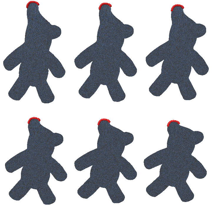
Here is the heat map applied to a shirt that was rigged using Maya’s copySkinWeights:

Here is the heat map applied to a shirt that was rigged using EpicGames Inpaint method:

Reference: EpicGames Inpaint Method

TextDeformer: How can words shape the (virtual) world

Researched by: José Pablo Soto Sánchez

Introduction

Imagine handing a sculptor a block of clay and, instead of tools, just a sentence: “make this a giraffe.” No reference photos, no measurements, just words, and the expectation that the clay reshapes itself to match. That’s roughly what TextDeformer (Gao et al., SIGGRAPH 2023) does to a 3D mesh: given a source shape and a target text prompt, it deforms the geometry until a frozen vision-language model agrees that the render looks like the prompt.

What makes this interesting isn’t just the result it’s used purely as a differentiable critic. The actual “learning” happens directly on the geometry: a set of per-triangle Jacobian matrices gets optimized by gradient descent, the same way you’d optimize the weights of a network, except here the “weights” are literally how each triangle is allowed to stretch and rotate.

This post walks through reproducing the official TextDeformer codebase end-to-end on consumer hardware, the math that makes text-to-geometry gradients possible at all, and the specific things that broke along the way and how they got fixed.

Background

A few terms are worth pinning down before the method section, since the pipeline sits at the intersection of graphics and vision-language modeling:

TermPlain-language definition
CLIPA frozen, pretrained model that embeds images and text into the same vector space, so cosine similarity between an image embedding and a text embedding measures “how well does this image match this caption.”
Differentiable renderingTurning a 3D mesh + camera into a 2D image using operations (rasterization, shading) that support backpropagation, so pixel-level loss can flow gradients back to vertex positions.
Jacobian (per-triangle)A 3×3 matrix describing how a single triangle is locally stretched/rotated relative to its original shape. TextDeformer optimizes one of these per face, directly.
Poisson mesh reconstructionGiven a target Jacobian per triangle, solving a linear system to recover the vertex positions whose actual local deformation best matches those targets, in a least-squares sense.
Cotangent LaplacianA sparse matrix built from mesh geometry that encodes how each vertex relates to its neighbors; it’s the operator at the center of the Poisson solve.
ViT patchA Vision Transformer splits an image into fixed-size square tiles (“patches”) and treats each one like a token — patch size determines how fine-grained the model’s spatial resolution is.

Method

CLIP-guided losses

The core signal is cosine similarity between a rendered image’s CLIP embedding and the target text’s CLIP embedding:

Δclip=cos(fimg(I^)fimg(Ibase),  ftext(target)ftext(base))\mathcal{L}_{\Delta\text{clip}} = -\cos\big(f_{\text{img}}(\hat{I}) – f_{\text{img}}(I_{\text{base}}),\ \ f_{\text{text}}(\text{target}) – f_{\text{text}}(\text{base})\big)

But optimizing this alone tends to drift toward whatever image maximizes similarity to the prompt, not necessarily a smooth deformation of the source shape. TextDeformer adds a delta-CLIP term that instead matches the change in image embedding against the *change* in text embedding, relative to a fixed base render/prompt (e.g. “a cow”):

clip=cos(fimg(I^), ftext(“a giraffe”))\mathcal{L}_{\text{clip}} = -\cos\big(f_{\text{img}}(\hat{I}),\ f_{\text{text}}(\text{“a giraffe”})\big)

This directional formulation (used in prior CLIP-guided editing work) keeps the deformation anchored to the source identity instead of collapsing onto an unrelated “giraffe-like” blob.

Per-triangle Jacobians and the Poisson solve

This is the part that replaces a neural decoder entirely. Given the mesh’s gradient operator GG (one 3×3 block per face) and a diagonal mass matrix MM of face areas, the cotangent Laplacian is built as:

L=GMGL = G^\top M G

LL has a one-dimensional null space (constant functions), so the implementation drops the first row/column to pin a single vertex before it’s usable for Cholesky factorization. To go from optimized per-face Jacobians JJ back to vertex positions vv, the code solves the normal equations of a least-squares problem — find the vv whose actual gradient GvGv is as close as possible to the target Jacobians JJ, weighted by face area:

v=argminvGvJM2Lv=GMJv^* = \arg\min_v \| Gv – J \|_M^2 \quad\Longrightarrow\quad L\, v = G^\top M J

That linear system is factorized once per mesh with a sparse Cholesky solver (`cholespy`, GPU-resident) and re-solved every optimization step as JJ changes — cheap after the one-time factorization. A Jacobian regularization term, JI2\| J – I \|^2, keeps triangles from stretching into degenerate shapes.

Rendering and camera augmentation

Each step, a batch of random cameras (elevation drawn from a Beta distribution, azimuth uniform over 360°, random distance/FOV/lighting/background) renders the current mesh via nvdiffrast‘s differentiable rasterizer. Randomizing viewpoint and lighting every step is what prevents the optimizer from exploiting a single “good” camera angle instead of actually deforming the geometry.

Patch-level consistency loss

A second, separate CLIP ViT is used only for its intermediate patch features (via forward hooks on each transformer block). For pairs of cameras within the same batch that are close in elevation/azimuth, the patches that project to the same 3D vertex are compared — encouraging the same surface point to look consistent from nearby viewpoints, which curbs the multi-view incoherence (“Janus-face”-style artifacts) common to CLIP-guided 3D optimization.

Implementation

Getting the reference implementation running at all. 

The repo pins specific commits for nvdiffrast and installs igl unpinned via conda-forge. The unpinned igl immediately caused a break: igl.random_points_on_mesh  in  MeshProcessor.py expected a 2-tuple return (bary, face_idx), but the installed libigl build now returns a 3-tuple (B, FI, P). Fixed by unpacking a third, unused value — a reminder that “no version pin” in a 2023 paper repo means the API surface has already drifted.

Fighting the GPU context, not the geometry. 

The next failure had nothing to do with the algorithm:  dr.RasterizeGLContext() threw cudaGraphicsGLRegisterBuffer (CUDA error 304, cudaErrorOperatingSystem) on first render. [VERIFY: root cause inferred from the error code and hybrid-GPU laptop symptoms, not confirmed via driver-level logs] — the working hypothesis is that Windows was creating the OpenGL context on the integrated GPU while CUDA ran on the discrete GPU, breaking the CUDA↔GL interop nvdiffrast relies on. The pinned nvdiffrast commit doesn’t expose the pure-CUDA rasterizer (RasterizeCudaContext isn’t present in this build), so the fix was OS-level: explicitly forcing the Python process to the discrete GPU in Windows’ graphics settings, rather than a code change.

Finding the actual VRAM ceiling. 

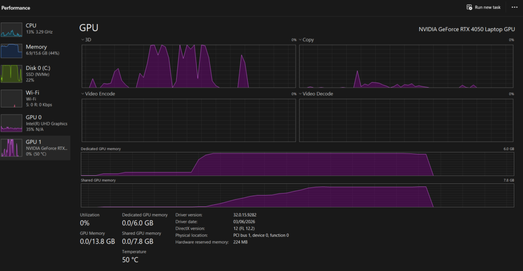
With rendering working, the default config (batch_size=25train_res=512) ran out of memory on a 6 GB laptop GPU (RTX 4050) partway through the first step. The batch dimension and the render resolution both scale memory close to linearly, so both got reduced (batch_size=4train_res=256) until a full 2,500-step run completed without OOM. This became the baseline configuration for every later experiment.
Swapping CLIP backbones without breaking assumptions baked into the code. 

clip_model and consistency_clip_model are independently configurable, but the consistency-loss implementation (utilities/clip_spatial.py) hardcodes assumptions that only hold for the “Base” ViT variants: a for i in range(12) loop over transformer blocks (ViT-L/14 has 24), and an assertion that the patch stride evenly divides the patch size (ViT-L/14‘s 14px patch isn’t divisible by the default stride of 8, unlike 32px/16px). RN50 — a convolutional backbone — can’t be used for the consistency loss at all, since that code depends on ViT-style patch tokens that a ResNet simply doesn’t produce. ViT-B/32ViT-B/16, and RN50 (as the primary loss only) were compared under an identical seed/mesh/prompt to keep the comparison controlled; ViT-B/32 was kept as the default going forward, primarily because it fit the VRAM budget without further code changes.

Debugging a mesh, not the code.

A custom tuna.obj mesh failed with CHOLMOD: not positive definite inside the Cholesky factorization. The Laplacian LL is only positive-definite after pinning one null-space direction — which is correct for a single connected mesh, but insufficient if the mesh has multiple disconnected components (each contributes its own null direction). The tuna model’s eyes turned out to be separate, unwelded geometry. Diagnosing this required leaving the codebase entirely and going into Maya: using Mesh → Separate to count connected shells, Combine + Merge (vertex welding by distance) to attempt reattachment, and re-running Separate as the verification step (if it can no longer split the mesh, it’s genuinely one piece). Welding never fully closed the gap without visibly displacing the eyes during remeshing, so the pragmatic fix was deleting the eye geometry outright, producing tunaNoEyes.obj — a reminder that not every mesh bug is worth solving at the mesh level when the pipeline’s actual requirement (single connected component) can be satisfied more simply.

Stale caches and unattended runs.

MeshProcessor caches differential operators and Jacobian .npz files under <output_path>/tmp/ and silently reuses them if present — convenient for resuming, dangerous if the source mesh changes but the output path doesn’t: a later run against a re-exported (different vertex count) tuna.obj crashed in a sparse matrix multiply because the cached operators no longer matched. Once that class of bug was understood, a small driver script (run_batch.py) was written to chain multiple mesh/prompt runs sequentially — the single 6 GB GPU rules out any parallelism — each with a fresh output directory and its own log file, so a several-hour unattended batch could run overnight without one failed run silently corrupting the next.

Results

Five source→target pairs were run to completion on the final configuration (batch_size=4train_res=256ViT-B/32, single RTX 4050 Laptop GPU):

Source → TargetStepsWall-clock
cow → giraffe (spot.obj)5,0001h 14m
fish → shark10,0002h 37m
eiffel tower → rocket10,0003h 21m
tuna → shark (tunaNoEyes.obj, remeshed)10,0002h 33m
guitar → axe6009m 39s

Per-step cost stayed in a fairly narrow band (~0.89–1.2 s/step) across meshes of similar triangle count, and scaled with batch_size × train_res as expected from the rendering cost analysis above — the guitar → axe run at 600 steps was deliberately short (~10 minutes) as a fast-iteration sanity check rather than a converged result, and looks correspondingly less refined than the 10k-step runs.

Future Work

Validate mesh topology before the Poisson solve, not during it. 

The tuna.obj failure surfaced as a Cholesky exception deep inside training, three layers of traceback away from the actual cause (disconnected components). A pre-flight check — counting connected components with igl and failing fast with a clear message before any GPU work starts — would turn a confusing runtime crash into an immediate, actionable one, and is a small, self-contained addition to MeshProcessor.py.

Generalize the consistency-loss encoder beyond the “Base” ViT assumption. 

The hardcoded 12-layer loop and stride-divisibility requirement in clip_spatial.py make ViT-L/14 unusable for the consistency loss without a code change, and rule out testing community-trained checkpoints (e.g. LAION’s ViT-B-32 retrained on LAION-2B via open_clip) that share the same architecture but arrive through a different loading path than OpenAI’s clip package. Both are architecture-family limitations, not fundamental ones — worth fixing before running a broader backbone ablation.

Reference

https://threedle.github.io/TextDeformer

ShapeFlow: Morphing Between 3D Shapes

We also explored a method for morphing one 3D shape into another target 3D shape. We worked with ShapeFlow, a neural network that learns to deform an existing 3D shape into another through a continuous flow field. Given latent space encodings of a source and target shape, the model outputs a velocity field describing how each point on the source should move to arrive at the target. Because the flow is continuous and (under the right conditions) bijective, the resulting deformation is guaranteed to be free of self-intersections, and can optionally preserve volume. Both of these properties can be desirable for artists working with meshes, which makes ShapeFlow attractive for toolification.

The Model

ShapeFlow’s creators frame the deformation of source shape XiX_i into target shape XjX_j as an advection process–the movement of a conserved property through fluid flow. Each point xx on the source is carried along a flow field f(x,t)f(x,t) over an interpolation parameter t[0,1]t\in[0,1]. Then, the points of the deformed source shape ϕij\phi_{ij} are described as:

Φij(x)=x(1), where x(t)=x(0)+0tfij(x(τ),τ)dτ\Phi_{ij}(x)=x(1) , \text{ where } x(t)=x(0)+\int_0^t f_{ij}(x(\tau),\tau)\;d\tau

Training seeks the mapping Φθij\Phi_{\theta}^{ij} that minimizes the symmetric Chamfer distance between the deformed source and the target:

minθC(Φθij(Xi),Xj)+C(Xi,Φθji(Xj))min_\theta \quad C(\Phi_{\theta}^{ij}(X_i), X_j) + C(X_i, \Phi_{\theta}^{ji}(X_j))

So the output of ShapeFlow is this flow field or mapping Φθij\Phi_{\theta}^{ij} that describes how each point on the source shape should advect in order for the source to become the target shape. How are the inputs to ShapeFlow created? What do we feed to the model?

Recall, we said that the input to ShapeFlow is the pair of latent space encodings from the source and target shapes. For our implementation, we use an encoder that maps a mesh’s vertices to a latent space encoding using a single forward pass. The encoder is trained jointly with the deformer model, using the same Chamfer distance loss, so it learns to produce encodings that are useful for conditioning the flow field.

The Toolification

Our goal was to implement ShapeFlow as a Maya plug-in for artists’ use in stylization and retopology of one mesh to another. To increase usability, we added blendshapes between the source mesh and the deformed source mesh by extracting and exporting intermediate results along the deformation path (sampling ϕij(x)ϕ_{ij}(x) at intermediate values of tt). This way, an artist can scrub through the flow and select whichever stage best fits their needs.

Future Exploration & Improvement

While implementing ShapeFlow as a Maya tool for artists, we ran into some areas of exploration for the performance of the tool. With more time we would have done more experimenting and development to ensure the model’s capabilities are consistent and high-performing for our desired use cases. On the SGI timeline we ultimately decided to balance exploration and execution and forge ahead with building out the tool while noting areas for improvement:

  • Initialization Sensitivity: Since the initialization of the model weights are random, results can vary widely based on whether one initialization was “good” for the specific meshes being used.
  • Loss Function Limitations: One of the use cases we wanted to develop ShapeFlow for was to create intermediate expressions for a given face mesh with certain extreme expressions. However, when morphing between meshes that differ only in a small region–for example puckered lips vs. a neutral expression–the region may be too small to affect the Chamfer distance loss during optimization. Other loss functions are worth evaluating for these cases.
  • Pretraining: If there are certain use cases (classes of objects, faces) that ShapeFlow will be used for, it might be beneficial to do pretraining on those types of shapes. Currently, our tool trains the deformer model from scratch every time. (This is also why the initialization sensitivity affects the results so strongly.) As a result, the model either will take an extremely long time with an appropriate amount of training iterations, or be used after a lower number of training iterations with reduced fidelity.

We did some manual tuning to get workable results on our test meshes, but making this robust enough for an artist’s workflow requires additional experimentation, testing, and development.

Results

Below is a video demonstrating the Maya tool workflow. For the sake of time, in the video the model is only trained for 200 iterations (very low), which is one source of the poor or unfinished-looking output flow.

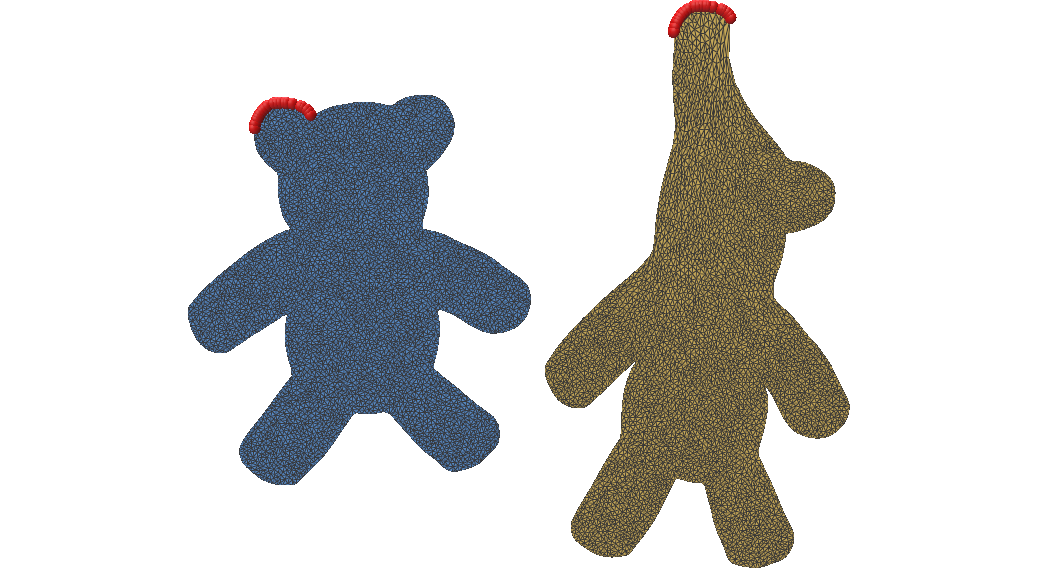
Below is an image showing how ShapeFlow can be used to produce a blend of two meshes. The ShapeFlow output (middle) is result of Toilet 1 (left) morphing into toilet 2 (right).

Reference

ShapeFlow

Categories
Research

Linear Subspace Exploration for Mechanical Systems

Project Members: Al Rahim Hossain, Stephanie Jung, Aleksa Milovanović, Reid Tang

Mentors: Otman Benchekroun, Ty Trusty

Introduction

Simulating deformable objects often requires optimizing over a large number of unknowns. For example, a 2D mesh with nn vertices has 2n2n positional variables: an xx and yy coordinate for each vertex. A 3D mesh similarly has 3n3n positional variables.

In a full order model, the deformed shape is represented by a vector 𝐱\mathbf{x} containing all vertex positions. It is found by minimizing the total energy of the object:

𝐱=argmin𝐱(Eelastic(𝐱)+Eext(𝐱))\mathbf{x}^*=\underset{\mathbf{x}}{\text{argmin}}\left(E_{\mathrm{elastic}}(\mathbf{x})+E_{\mathrm{ext}}(\mathbf{x})\right)

where EelasticE_{\mathrm{elastic}} measures how much the object resists being deformed from its rest shape and EextE_{\mathrm{ext}} represents external forces. The solution 𝐱\mathbf{x}^* is the state with the lowest total energy, where the elastic response and external forces are balanced. However, this solution may be computationally expensive as it treats every vertex position as an independently moving variable.

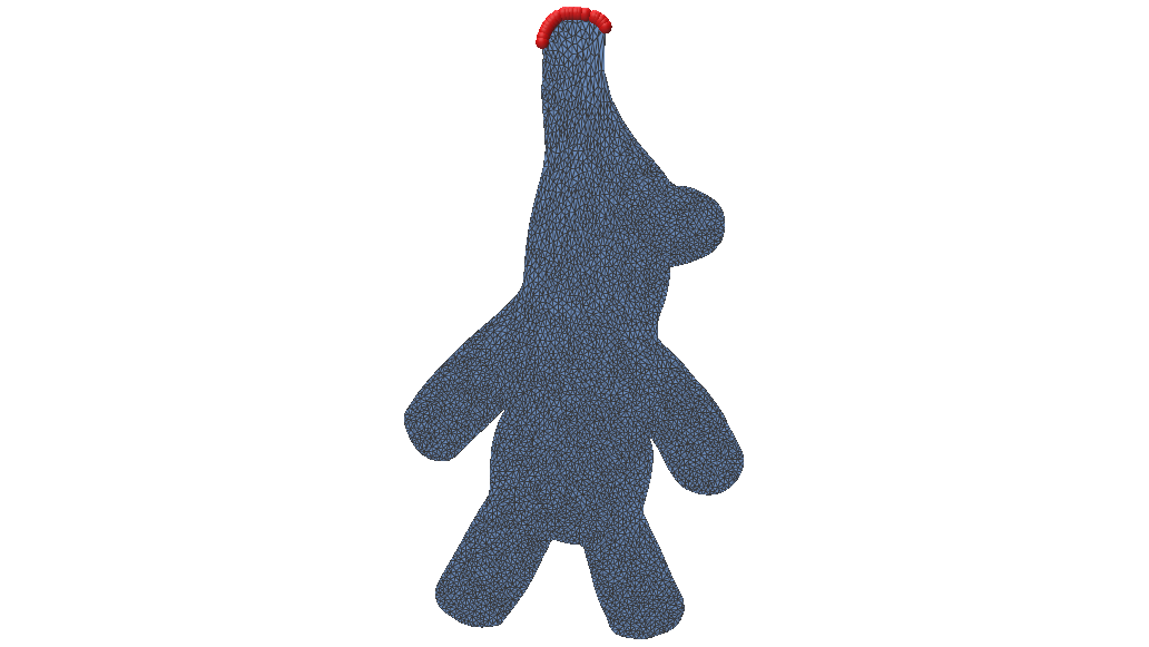
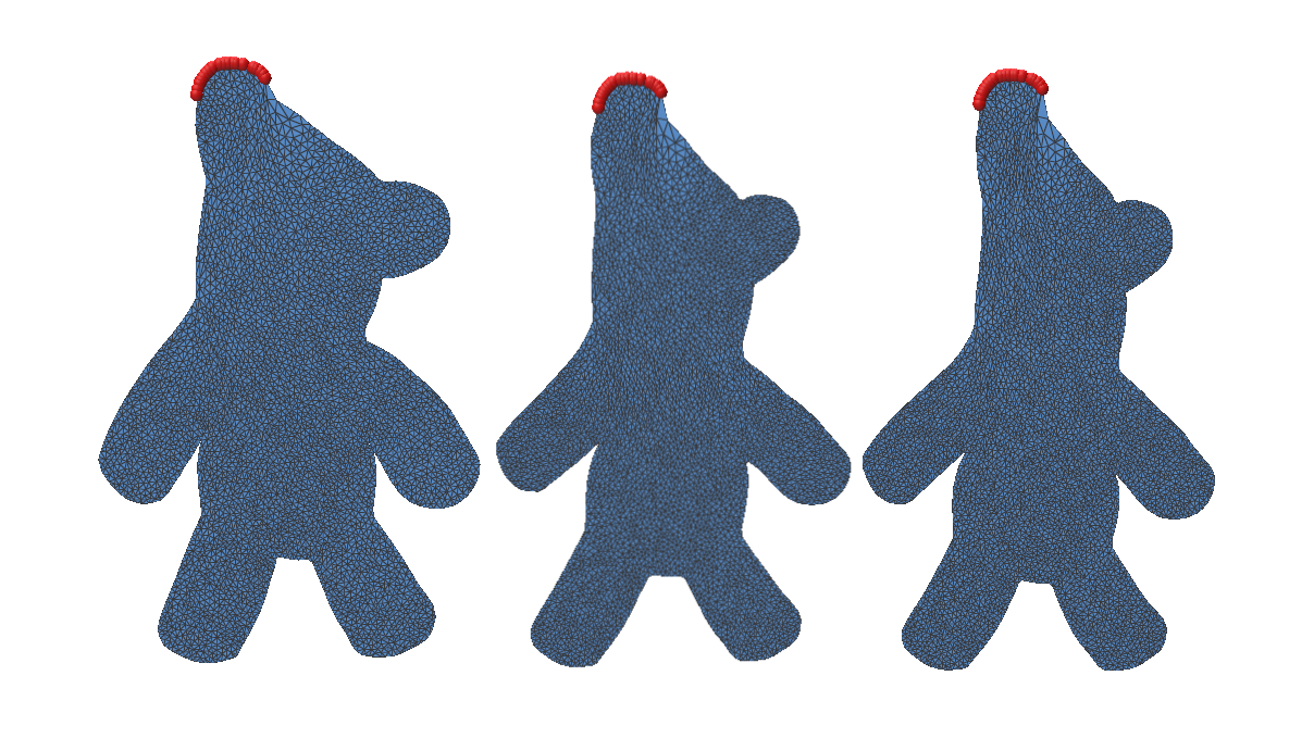
Figure 1: Comparison of the original 2D mesh (left) and its Neo-Hookean deformation (right) under gravity (g=0.1g = -0.1), with fixed vertices highlighted in red. This represents the exact solution 𝐱\mathbf{x}^* found using Newton’s method.

Reduced-Order Model

Reduced-order modelling reduces the size of this optimization by restricting the solution to a low-dimensional subspace. Instead of tracking every point independently, we choose a small set of meaningful deformation patterns. We then approximate the full configuration as 𝐱𝐱𝟎+𝐁𝐳\mathbf{x} \approx \mathbf{x_0 + Bz} where 𝐱𝟎\mathbf{x_0} is the rest state of the object, the columns of matrix 𝐁\mathbf{B} represent the selected deformation patterns, and vector 𝐳\mathbf{z} contains their corresponding coefficients [1]. We can now solve for

𝐳=argmin 𝐳E(𝐱𝟎+𝐁𝐳)\mathbf{z}^* = \underset{\mathbf{z}}{\text{argmin }}E(\mathbf{x_0 + Bz})

and the final full-space solution is given by 𝐱𝐱𝟎+𝐁𝐳\mathbf{x}^* \approx \mathbf{x_0 + Bz}^*.

The effectiveness of a reduced-order model depends heavily on the choice of the basis 𝐁\mathbf{B}. Ideally, its columns should capture the important deformation patterns of the object using as few modes as possible. There are several ways to construct such a basis.

Proper Orthogonal Decomposition

Proper Orthogonal Decomposition constructs the basis from a dataset of observed or simulated deformations [2]. It finds the directions that best capture the variation present in the example shapes, making it a data-driven approach. It is found by solving

𝐁=argmin 𝐁||𝐗𝐁𝐁T𝐗||2\mathbf{B} = \underset{\mathbf{B}}{\text{argmin }} ||\mathbf{X – BB}^T\mathbf{X}||^2 such that 𝐁T𝐁=𝐈\mathbf{B}^T\mathbf{B=I}

Here, 𝐗\mathbf{X} is a matrix whose columns contain example displacement vectors from the rest configuration of the object. We use singular value decomposition, 𝐗=𝐔𝐒𝐕T\mathbf{X} = \mathbf{USV}^T, to find the deformation patterns that best represent these examples. The columns of 𝐔\mathbf{U} are ordered from most to least important so if we want a reduced space with 20 modes, for example, we simply take the first 20 columns 𝐁=𝐔[:,:20]\mathbf{B} = \mathbf{U}[:, :20].

Figure 2: Top: Full-order solutions with gravity g[0.002,0.003,0.004,0.005,0.006,0.007]g \in [-0.002, -0.003, -0.004, -0.005, -0.006, -0.007] used to form the dataset. Bottom: Deformation under gravity g=0.1g = -0.1 using POD. Fixed vertices highlighted in red.

A main drawback of POD is that it requires collecting a representative set of deformation examples beforehand. The resulting subspace can only represent deformation patterns present in, or similar to, this training data, so unseen motions may be captured poorly.

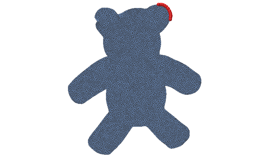
Figure 3: Deformation under gravity g=0.1g = -0.1 using the POD basis from Figure 2 but with fixed vertices on the opposite ear. It fails since this configuration is not represented in the basis.

Linear Modal Analysis

Linear Modal Analysis builds the reduced basis from the object’s natural vibration modes around its rest shape [3]. The basis vectors are deformation modes obtained from the mesh’s stiffness and mass matrices, so the subspace is determined by the physics of the object rather than by example deformation data. These modes are found by solving the generalized eigenvalue problem

𝐇ϕ=λ𝐌ϕ\mathbf{H}\phi = \lambda\mathbf{M}\phi.

Here, 𝐇\mathbf{H} is the elastic stiffness of the object and 𝐌\mathbf{M} accounts for its mass. Solving the eigenvalue problem gives the natural deformation patterns ϕ\phi, or modes, of the object. The lowest-frequency modes are usually the most important and are chosen as the columns of the reduced basis 𝐁\mathbf{B}.

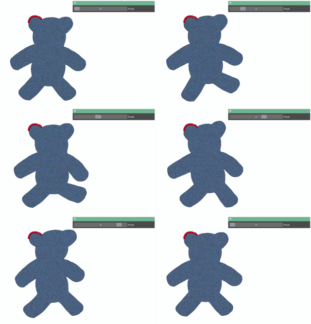
Figure 4: Top: Animation of the first 10 deformation modes. Bottom: Deformation under gravity g=0.1g = -0.1 using an LMA basis with 5 modes (left), 10 modes (center), and 20 modes (right).
However, LMA is based on a linearization around the rest shape, so it works best for small deformations. Large rotations or strongly nonlinear deformations may not be represented well by a basis of linear vibration modes.

Actuation-Aware Subspaces

POD can capture large deformations, but it requires representative simulation data. LMA avoids this data collection, but its basis is not aware of the parameters driving the simulation. Actuation-aware subspaces build the reduced basis directly from how the object deforms as the actuation parameters change. We write

𝐱(𝐚)=argmin 𝐱E(𝐱,𝐚)\mathbf{x(a)} = \underset{ \mathbf{x} } { \text{argmin } } E(\mathbf{x, a})

where 𝐚\mathbf{a} may represent quantities such as spring rest lengths, gravity, muscle activation, or collider parameters. The goal is to approximate how 𝐱(𝐚)\mathbf{x(a)} changes as 𝐚\mathbf{a} changes.

We can first approximate this relationship using a first-order Taylor expansion around a reference actuation 𝐚0\mathbf{a}_0:

𝐱(𝐚)𝐱(𝐚0)+i(aia0,i)𝐱ai\mathbf{x}(\mathbf{a})\approx\mathbf{x}(\mathbf{a}_0)+\sum_i(a_i-a_{0,i})\frac{\partial\mathbf{x}}{\partial a_i}.

The derivatives 𝐱ai\frac{\partial \mathbf{x}}{\partial a_i} describe the deformation caused by changing each actuation parameter. For example, if the object is driven by springs, each parameter could control the rest length of one spring. However, this is still a linear approximation and works best for small deformations near 𝐚0\mathbf{a}_0. Larger motions such as bending, rotation, and compression follow curved deformation paths that cannot be represented well using only fixed linear directions.

To capture these effects, we include second-order derivatives, 2𝐱aiaj\frac{\partial^2 \mathbf{x}} {\partial a_i \partial a_j}, for the second-order Taylor expansion:

𝐱(𝐚)𝐱(𝐚0)+i(aia0,i)𝐱ai+12ij(aia0,i)(aja0,j)2𝐱aiaj\mathbf{x}(\mathbf{a}) \approx \mathbf{x}(\mathbf{a}_0) + \sum_i (a_i-a_{0,i}) \frac{\partial \mathbf{x}}{\partial a_i} + \frac{1}{2} \sum_i\sum_j (a_i-a_{0,i})(a_j-a_{0,j}) \frac{\partial^2 \mathbf{x}}{\partial a_i \partial a_j}

If the first derivatives describe the response to actuation, the second derivatives describe how that response changes as the actuation changes. These terms help capture deformation patterns that appear together during larger motions, allowing the reduced space to follow nonlinear deformation paths more closely.

The reduced subspace can therefore be formed by

𝐁=[𝐱a1  𝐱ap 2𝐱a12  2𝐱aiaj]\mathbf{B} = \left[ \frac{\partial \mathbf{x}}{\partial a_1} \ \cdots\ \frac{\partial \mathbf{x}}{\partial a_p} \ \frac{\partial^2 \mathbf{x}}{\partial a_1^2} \ \cdots\ \frac{\partial^2 \mathbf{x}}{\partial a_i \partial a_j} \right]

such that this space is tailored to the parameters driving the simulation.

This idea is similar to modal derivatives [1], which describe how linear vibration modes change and interact. Here, we apply the same idea to actuation parameters, so the basis is tailored to the forces that will actually drive the simulation.

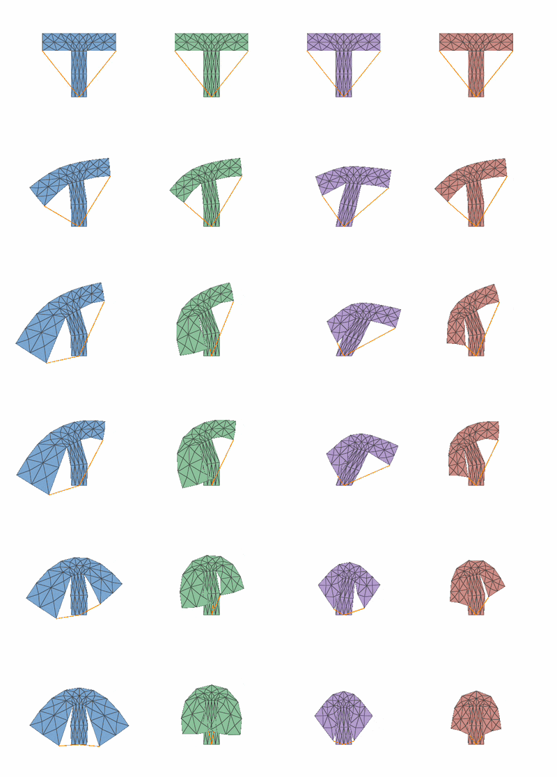
Figure 5: Deformation under spring actuation as the spring is made tighter using (from left to right): first-order approximation, second-order approximation, LMA, and an exact solution using Newton’s method.
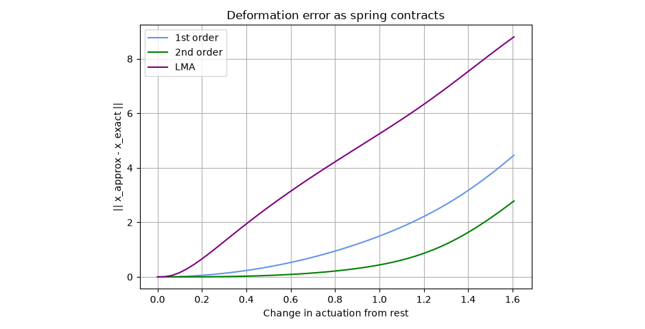
Figure 6: Deformation error as the spring contracts for the first-order, second-order, and LMA reduced models compared with the exact solution.

Conclusion

Reduced-order models can make deformable simulations more efficient by representing motion with a small number of deformation patterns. In this project, we explored an actuation-aware basis that is built from how the equilibrium shape changes with the parameters driving the simulation. First-order derivatives capture the main response to actuation, while second-order derivatives help represent larger and more nonlinear deformations.

There are still several directions for future work. Hyper-reduction is needed to further reduce computational cost [4], and the current method relies on a PSD-projected Hessian for stable basis construction. The number of basis terms also grows with the number of actuation parameters. Future work could address these limitations and extend the method to more complex 3D scenes and different types of actuation.

References

[1] J. Barbič and D. L. James. Real-Time Subspace Integration for St. Venant-Kirchhoff Deformable Models. ACM Transactions on Graphics, 2005.

[2] L. Sirovich. Turbulence and the Dynamics of Coherent Structures. I. Coherent Structures. Quarterly of Applied Mathematics, 45(3), 561–571, 1987.

[3] A. Pentland and J. Williams. Good Vibrations: Modal Dynamics for Graphics and Animation. SIGGRAPH, 1989.

[4] C. Brandt, E. Eisemann, and K. Hildebrandt. Hyper-Reduced Projective Dynamics. ACM Transactions on Graphics, 2018.

Categories
Research

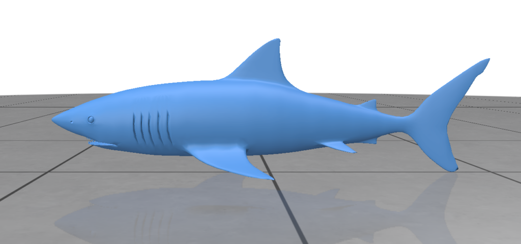
Teaching a Mesh Which Way to Swim: Intrinsic Triangulations and the Anisotropic Laplacian

Introduction

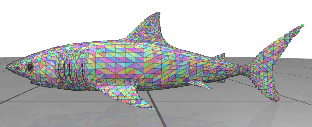
Swimming with a current feels effortless; swimming across it is exhausting — even over the same distance in meters. That asymmetry isn’t a fact about water, it’s a fact about which notion of “distance” you’re using. This week’s project builds exactly that idea into a triangle mesh: a metric that makes some directions cheaper to move through than others. Along the way we needed two core tools from discrete differential geometry — intrinsic triangulations and the anisotropic Laplacian — and had to make both of them survive a real 3D shark scan, not just a hand-drawn toy mesh.

Background

A quick glossary before the derivations:

  • Mesh (V, F): vertex positions and the triangles connecting them.
  • Halfedge: a directed half of an edge, belonging to one triangle; its twin is the matching half from the triangle on the other side. This lets code ask “what’s across this edge?” in constant time.
  • Tensor field / metric S: a small symmetric, positive-definite matrix per triangle (2×2 in 2D, 3×3 on a 3D surface) describing how expensive movement is in each direction. S = I recovers ordinary Euclidean distance.
  • Intrinsic triangulation: a different triangulation of the same surface, changing only connectivity — never vertex positions.
  • Edge flip: the only move allowed — swap the diagonal of the quad formed by two triangles sharing an edge.
  • Delaunay triangulation: every edge satisfies the empty-circumcircle property; avoids thin, needle-like triangles.
  • Cotangent weight (wij): built from the two angles opposite an edge; decides both whether to flip it and what enters the Laplacian.
  • Harmonic field: a function solving Lf=0Lf=0 with fixed boundary values — “ink diffusing smoothly” between two fixed points.

Method: Intrinsic Triangulations

An intrinsic triangulation keeps a mesh’s lengths and angles — what an ant walking on the surface could measure — while reconnecting vertices via edge flips:

  i                 i
 /|\               / \
/ | \             /   \
m |  k   ====>   m --- k
\ | /             \   /
 \|/               \ /
  j                 j

This matters because it can fix badly-shaped triangles without adding a single vertex — useful whenever an algorithm only needs lengths and angles, not raw coordinates.

The special case is the Delaunay triangulation, equivalent to:
wij=12(cotα+cotβ)0    α+β180°w_{ij} = \tfrac12(\cot\alpha+\cot\beta) \geq 0 \iff \alpha+\beta \leq 180°

The proof is short: cotα+cotβ=sin(α+β)sinαsinβ\cot\alpha+\cot\beta = \frac{\sin(\alpha+\beta)}{\sin\alpha\sin\beta}​, and since α,β(0°,180°)\alpha,\beta\in(0°,180°) the denominator is always positive — so the sign of wij​ depends only on sin(α+β). Empty-circumcircle and angle-sum are the same condition. In code, this is a queue: flip any edge with negative weight, re-check its neighbors, repeat until none remain.

Method: The Anisotropic Laplacian

To make distance direction-dependent, attach a metric MMM to each triangle: vM=vMv\|v\|_M=\sqrt{v^\top Mv}​. M must be symmetric (for real eigenvalues/perpendicular axes) and positive-definite (so no length comes out negative or imaginary).

The pleasant surprise: the Delaunay proof above never used Euclidean angles specifically — only that they’re triangle angles in (0°,180°). Measuring α,β with M instead, the same algebra holds, so the criterion is unchanged in form. On a fixed test quad, switching S from identity to diag(1,16) flips the verdict entirely (w: +0.72 → -1.37) — same vertices, different verdict on whether the edge should exist.

The same wijw_{ij}​ assembles the Laplacian (Lij=wijL_{ij}=-w_{ij}, Lii=jwijL_{ii}=\sum_j w_{ij}​), which must satisfy: rows sum to zero, symmetric, constants in the kernel. When all wij0w_{ij}\geq0 (i.e., Delaunay), LL also satisfies the maximum principle — solutions to Lf=0Lf=0 extremize only on the boundary. That guarantee is the entire reason the flip exists before building anything on top of LL.

Implementation

The build order, including what broke:

Synthetic 2D test bed: HalfedgeMesh with flip_edge/flip_to_delaunay, validated on a hand-built non-Delaunay quad and a randomly-scrambled disc.

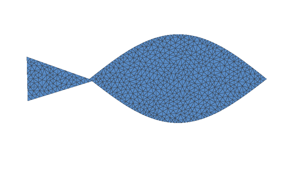
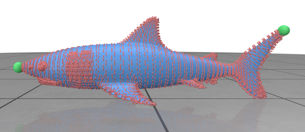
Toy 2D fish: solved a harmonic field (nose=0, tail=1) with the ordinary Laplacian, took its per-triangle gradient as the “body direction” dd, and built S=αdd+β(Idd)S=\alpha\,dd^\top+\beta(I-dd^\top), α<β\alpha<\beta— cheap along the body, expensive across it.

Real 3D shark scan — the actual porting work:

Cleanup: weld coincident vertices, drop degenerate (zero-area) faces, since these send cotangent weights to nan and corrupt connectivity.

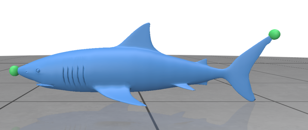
Automatic nose/tail: SVD on centered vertices finds the principal axis; nose and tail are its two extremes.

A genuinely 3D gradient: no single “perpendicular” exists on a surface, so the normal nn and cross product replace 2D rotation: f=12Aifi(n×ei)\nabla f = \frac{1}{2A}\sum_i f_i(n\times e_i), and the tensor grows to 3×3 with a transverse direction t=n×dt=n\times d.

Hardening the flip queue: index by (face, corner) instead of hashing mutable Halfedge objects; return None instead of nan for degenerate triangles; reject flips that would duplicate an existing edge.

Results

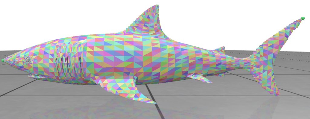
The Polyscope UI toggles between the original mesh and the re-triangulated one, with a live counter of non-Delaunay edges before/after and total flips performed. Recomputing the direction field after flipping shows the payoff: geometry never moved, but connectivity reorganized to better respect the metric — the field still tracks the shark’s body, now on better-conditioned triangles.

Categories
Research

Hyper dimension Editing

By Evelyn Zhu, Mentor: Alvin Shi,

Have you ever wondered what 4D actually looks like? I do, I have always imagined what will 4D world looks like, and in this project I was able to take a small peak at this enigmatic world.

But before I show you, there’s one thing I need to introduce first. Here’s the problem: we live in three dimensions. Our eyes, our screens, our intuition are all 3D. A four-dimensional object simply doesn’t fit into the world we’re able to look at. So how could we possibly “see” one?

The trick is to translate between dimensions. There are two operations that do exactly that: one to build a dimension up, and one to peek a dimension down. They’re called extrusion and slicing, and once you have them, 4D stops being impossible to picture [1].

Extrusion: building a dimension up

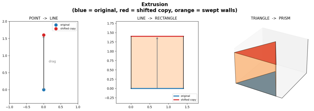
Extrusion is something you already know, even if you’ve never called it that. Take a shape, make a copy, drag the copy along a brand-new direction, and fill in everything it sweeps through. A point dragged becomes a line. A square dragged becomes a cube. And a 3D object dragged along a fourth axis becomes a genuine 4D object (See figure 1).

Figure 1: explain extrusion in 1D, 2D, and 3D respectively.

Every rung of that ladder climbs one dimension. The secret is the direction you drag: as long as it points along a fresh axis the shape wasn’t already using, you gain a dimension. Drag a cube in a direction perpendicular to width, height, and depth all at once — a direction we can’t even point at and we’vejust built a shape in 4D.

Slicing: peeking a dimension down

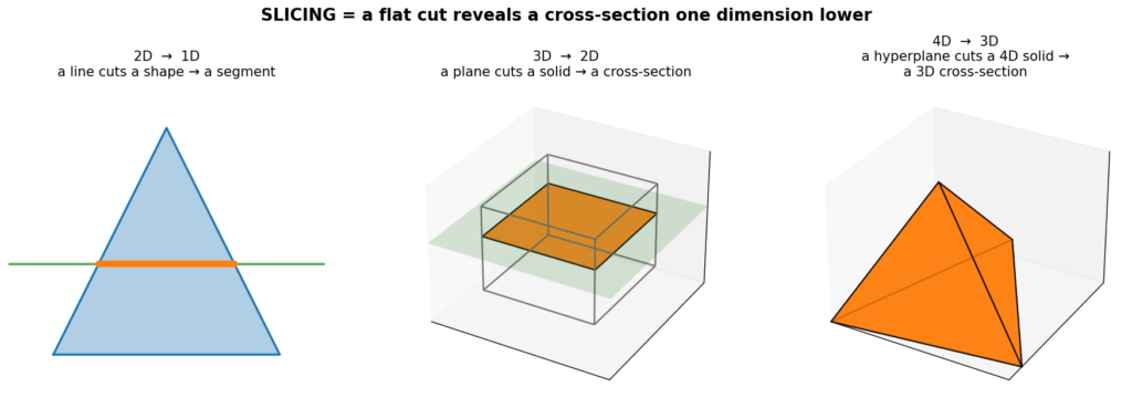
Slicing is the opposite move. Instead of building up, we cut across. Pass a flat plane through a solid, and where it cuts, you get a cross-section one dimension lower. Slice an 2D triangle, you get a line segment; slicing a 3D cube, you will get a 2D square (see figure 2).

Figure 2: explain slicing in 2D, 3D, and 4D respectively. orange represent the cross-section.

Now push that one rung higher: if we slice a 4D object with a “flat 3D plane” (a hyperplane), and the cross-section is a 3D shape, and this is finally something we can look at. That’s the whole idea. We can’t see the 4D object directly, but we can see its 3D slices.

Putting it together: watching 4D

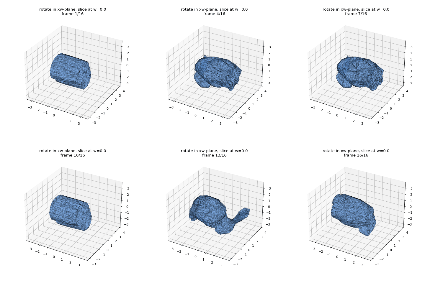
So here’s how we can actually “see” 4D object in our 3D world. We take a 4D objects and we slice it (1 dimension down). One slice gives one 3D snapshot. But a single snapshot isn’t enough to feel a 4D shape, so we do something more: we slowly rotate the object through the fourth dimension and re-slice it at every step.

Figure3: Each frame is a single 3D cross-section of a 4D object at fixed w. This mesh is the standford bunny.

Here’s exactly what you’re looking at, step by step:

  1. The object is 4D version of the stanford bunny. Every one of its points has four coordinates: the usual x, y, z, plus a fourth one we’ll call w. We can’t display it directly, because w points in a direction our world doesn’t have.
  2. We fix w and take the cross-section. Holding w at a single value, we ask: which parts of the object live exactly there? That set of points forms a 3D shape — one slice. This is the slicing operation, applied to every little piece of the object and stitched together into the shape you see.
  3. We rotate in 4D. Between frames, we turn the object by a small angle in a plane that involves w (here, the xw-plane). This is a true four-dimensional rotation, and it tips parts of the object that were “elsewhere along w” toward our fixed slice.
  4. We re-slice, and repeat. Because the rotation carries new material through the slice, each frame’s 3D cross-section differs from the last. Play the frames in sequence and the shape appears to be growing, shrinking, splitting, and merging.

And this is the whole magic trick: we use extrusion to build a 4D object from 3D object then slicing to see it. Two simple moves and now a dimension we were never supposed to be able to view suddenly becomes something we can sit back and watch.

References

[1] Alvin Shi, Haomiao Wu, and Theodore Kim. 2025. Hyper-Dimensional Deformation Simulation. In ACM SIGGRAPH 2025 Conference Papers. ACM. https://doi.org/10.1145/3721238.3730730

Categories
Research

Exploring Dependence Between Curvature and Heat Diffusion on a Mesh

By Shannon Cudworth, Mentors: Alek Fröhlich and Daniel Perazzo

Introduction

The goal of the project was to study statistical dependence from geometric perspective, where we define two random variables X, Y are defined on a surface \mathcal{M}, rather than in a Euclidean space. Specifically, we explore whether heat diffusion across a surface is dependent on the local curvature.

To study this relationship, we randomly sample a triangle face from a mesh and then construct one heat diffusion variable and one curvature variable for this sampled face. The former variable was defined using the Laplace-Beltrami operator, and for the latter variable we used the mean curvature value at the sampled face’s barycenter. We then employed the Hilbert–Schmidt Independence Criterion (HSIC) to investigate if faces with similar heat diffusion also have similar curvature.

To implement, we first sample faces with a probability proportional to their area, to avoid oversampling smaller triangles. After constructing the two aforementioned variables, we make curvature and heat kernel matrices to describe pairwise curvature and heat similarity, run a permutation test, and repeat for various sample sizes to estimate the power of the sample HSIC test.

Constructing the Heat Diffusion Variable

To approximate heat diffusion, we’re going to use the Laplace-Beltrami operator. For this, we need the cotangent Laplacian and mass matrix.

Cotangent Laplacian: A discrete approximation of the Laplace-Beltrami operator, used on triangle meshes. We define this matrix using the piecewise function:

Lij={12(cotαij+cotβij),ij, (i,j)E,k𝒩(i)12(cotαik+cotβik),i=j,0,otherwise.L_{ij} = \begin{cases} -\frac{1}{2}\left(\cot\alpha_{ij}+\cot\beta_{ij}\right), & i\neq j,\ (i,j)\in E,\\ \sum_{k\in\mathcal{N}(i)} \frac{1}{2}\left(\cot\alpha_{ik}+\cot\beta_{ik}\right), & i=j,\\ 0, & \text{otherwise.} \end{cases}

Where αij\alpha_{ij} and βij\beta_{ij} are opposite angles for the edge (ij), and N(i) is the set of neighboring vertices to vertex i.

Mass Matrix: Represents how much of the mesh’s surface area is associated with each individual vertex, and was defined using gpy toolbox.

With both of these components, we can understand the geometric variation of the mesh’s surface (through the Laplacian), and how much the variation contributes to the overall surface area of the mesh (though the Mass Matrix).

To actually approximate the heat diffusion over the area, we need to solve the eigenvalue problem:

Lϕi=λiMϕiL\phi_i = \lambda_iM\phi_i

where L is the cotangent laplacian, M is the mass matrix, ϕi\phi_i is the ith eigenvector, and λi\lambda_i is the corresponding ith eigenvalue.

Using Scipy, we solve for the first 100 eigenvector-eigenvalue pairs, which represents the 100 smoothest solutions to the equation above. The eigenvector defines a basis function over the mesh vertices, and the eigenvalue is the rate of decay under heat diffusion.

Now, to construct our random variable X, we must recall that we have sampled a random face of the triangle mesh, and we have two arrays eigenvectors and eigenvalues, where:

eigenvectors[i]
eigenvalues[i]

returns the first 100 eigenvectors and eigenvalues at vertex i of the mesh. To utilize these arrays, we must directly evaluate the eigenvalue problem at the sampled face’s barycenter. Then for the sampled face with vertices i,j,k we calculate:

(eigenvectors[i] + eigenvectors[j] + eigenvectors[k]) / 3

which gives us a vector of the form:

[ϕ1(bi)ϕ2(bi)ϕ100(bi)]\begin{bmatrix} \phi_1(b_i) \\ \phi_2(b_i) \\ \vdots \\ \phi_{100}(b_i) \end{bmatrix}

where bib_i is the barycenter of the ith sampled face.

Then using the respective eigenvalue, we can construct a random variable XiX_i that represents the heat diffusion from barycenter of the ith sampled face with:

Xi=[etλ1/2ϕ1(bi)etλ2/2ϕ2(bi)etλ100/2ϕ100(bi)].X_i = \begin{bmatrix} e^{-t\lambda_1/2}\phi_1(b_i) \\ e^{-t\lambda_2/2}\phi_2(b_i) \\ \vdots \\ e^{-t\lambda_{100}/2}\phi_{100}(b_i) \end{bmatrix}.
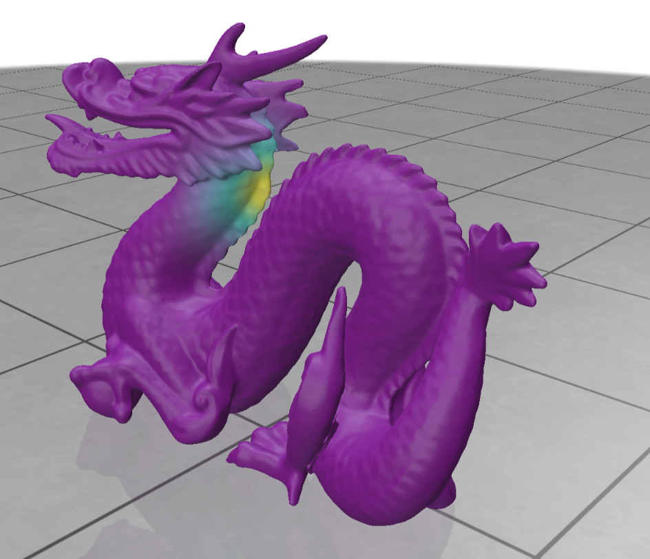
Figure: Heat diffusion from the barycenter of the sampled face on the dragon mesh

Constructing the Curvature Variable

To construct the curvature variable, we calculate the mean curvature at each of the sampled face’s three vertices. Using libigl’s principal curvature value function, we return k1, k2,k_1, \space k_2, the maximum and minimum curvature values at a vertex, respectively. We can then calculate the mean curvature value, defined as:

H=(k1+k2)2H = \frac{(k_1 + k_2)}{2}

If the mean curvature is small or 0, we can interpret either a locally flat surface, or a saddle structure where k1k_1 and k2k_2 cancel each other out. A larger mean curvature indicates bending.

Then for the ith sampled face with vertices i,j,k, we can construct the random variable YiY_i, which will calculate the curvature at the face’s barycenter, defined as:

Yi=H(bi)=(Hi+Hj+Hk)3Y_i = H(b_i) = \frac{(H_i + H_j + H_k )}{3}

where Hi, Hj, HkH_i,\space H_j, \space H_k are the mean curvature values at vertex i, j, k, and H(bi)H(b_i) is the mean curvature at the barycenter of the ith sampled face.

Kernels

To check independence between our two random variables X and Y, we must construct kernel matrices, which will measure the similarity between pairs Xi, XjX_i, \space X_j and Yi, YjY_i, \space Y_j (Schrab 19).

X variable: By construction of the laplacian, we can calculate the heat kernel KXK_X by:

KX=XXTK_X = XX^T

By definition:

Xi=[etλ1/2ϕ1(bi)etλ2/2ϕ2(bi)etλ100/2ϕ100(bi)].X_i = \begin{bmatrix} e^{-t\lambda_1/2}\phi_1(b_i) \\ e^{-t\lambda_2/2}\phi_2(b_i) \\ \vdots \\ e^{-t\lambda_{100}/2}\phi_{100}(b_i) \end{bmatrix}.

Then we can say for any i,j:

XiXj==1100(etλ/2ϕ(bi))(etλ/2ϕ(bj))X_{i}X_{j}^{\top} = \sum_{\ell=1}^{100} \left( e^{-t\lambda_\ell/2}\phi_\ell(b_i) \right) \left( e^{-t\lambda_\ell/2}\phi_\ell(b_j) \right)

Then,

XiXj==1100etλϕ(bi)ϕ(bj)X_{i}X_{j}^{\top} = \sum_{\ell=1}^{100} e^{-t\lambda_\ell}\phi_\ell(b_i) \phi_\ell(b_j)

which is the heat kernel formula (Mostowsky et al.).

Y variable: Unlike the heat diffusion variable X, we need to do a few more calculations to compute the curvature kernel KYK_Y, which we will do by using the Gaussian Kernel formula.

First, we define σY\sigma_Y, which represents the median pairwise distance for each Yi, YjY_i,\space Y_j pair. Then we can calculate the kernel KYK_Y using the formula, for each i,j pair:

KY(i,j)=exp(||YiYj||22σY2)K_Y(i,j) = exp(-\frac{||Y_i – Y_j||^2}{2\sigma_Y^2})

If KX, KYK_X, \space K_Y are large, then it follows that the ith and jth sampled faces have similar diffusion or similar curvature, respectively. Rather, if the kernels are small, then we can say the ith and jth sampled faces have different diffusion or curvature, respectively.

Hilbert-Schmidt Independence Criterion (HSIC)

The kernel matrices KX,KYK_X, K_Y allow us to determine if there are any similarities between pairs Xi, XjX_i, \space X_j or Yi,YjY_i, Y_j. Now, we want to examine that if pair Xi,XjX_i, X_j are similar, if it is true that pair Yi,YjY_i, Y_j are similar as well. To acheive this, we compute the sample HSIC.

To ensure valid comparability between variables, we first make a centering matrix, defined as:

H=Inxn1nJnxnH = I_{nxn} – \frac{1}{n}J_{nxn}

where JnxnJ_{nxn} is a matrix of all ones.

We can then define the centered kernels for X and Y as:

KXC=HKxH KYC=HKYHK_{XC} = HK_xH \\\\\\\\\\\\\ K_{YC} = HK_YH

Then, by definition,

HSIC(KX,KY)=1(n1)2tr(KXCKYC)HSIC(K_X,K_Y) = \frac{1}{(n-1)^2}tr(K_{XC}K_{YC})

Here, a large sample HSIC value indicates dependence between heat diffusion and curvature (Schrab 25).

Permutation Testing and Power

One sample HSIC value isn’t enough to statistically determine whether or not X, Y have dependence. So, we must undergo a permutation test. To start, we define a null and alternative hypothesis:

H0:X,Y are independentHA:X,Y are dependentH_0: X, Y \space are \space independent \\ H_A: X, Y \space are \space dependent

Our goal for this test is to simulate under the null hypothesis, and then see how likely our originally observed sample HSIC is to occur in those conditions. We permute the order of KYK_Y, recompute the sample HSIC, and repeat 200 times to create the null distribution. We then use the observed sample HSIC to calculate a p-value, which indicates whether or not we should reject or fail to reject the null hypothesis.

Taking a step further, we calculated the power of the sample HSIC test, which will give us the probability that, when X and Y are dependent, the sample HSIC will correctly detect that dependence. We do this by repeating the permutation test, and dividing the amount of times we rejected the null (p-value was less than 0.05, depending on significance level) by the total amount of retrials.

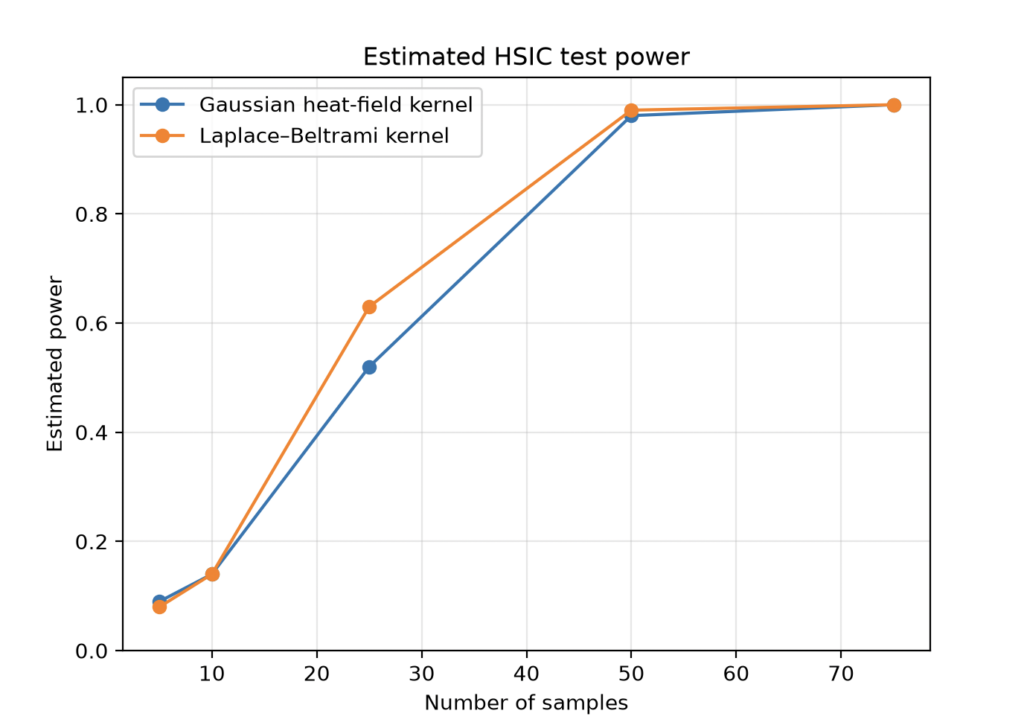
In our project, we compared the power of the sample HSIC test across sample sizes: 5, 10, 25, 50, 75, and repeated the permutation test 100 times per each sample size. We also compared the sample HSIC using the aforementioned heat diffusion kernel that was calculate with the Laplace-Beltrami operator, and another heat diffusion X variable and kernel, that was constructed using a numerical approximation and Gaussian Kernel method.

Figure: Shows the HSIC test power between random variables X,Y with a Gaussian heat diffusion kernel and Laplace-Beltrami heat diffusion kernel. Note that while the Laplace-Beltrami kernel does better for smaller samples, both converge to 1 as sample size increases.

From the figure, we can see that, as the sample size increases, the power of sample HSIC test equals 1. This means that every trial rejected the null hypothesis, and the sample HSIC test is successful at detecting dependence between heat diffusion and curvature.

Possible Extensions of the Project

I think it would be fun to compare the sample HSIC across different meshes, and maybe how quickly the power of the sample HSIC test converges to one across different meshes. We could also compare different curvature formulas with heat diffusion, or vary the time that we allow heat diffusion to occur. Or, we can explore with different variables, such as letting X represent the geodesic field from a sampled face, and compare that to curvature.

Works Cited

Schrab, Antonin. “Optimal Kernel Hypothesis Testing.” University College London, 2025.

Mostowsky, Peter, et al. “The GeometricKernels Package: Heat and Matérn Kernels for Geometric Learning on Manifolds, Meshes, and Graphs.” Journal of Machine Learning Research, vol. 26, no. 276, 2025, pp. 1–14.

odedstein. sgi-introduction-course. GitHub, https://github.com/ddecatur/sgi-introduction-course.

Categories
Research

Self-Rectifying Textures

By: Kyle Loh, Mahlet Girma, Max Dunitz

If you have ever had to flatten out a bag of chips so the checkout scanner would finally read it, you already understand the problem we worked on this week. A code printed on a surface that bends, folds, or curves is hard to read, and QR codes and barcodes carry one disadvantage here: they are obvious. In supply-chain tracking, that single visible code can be tampered with, causing a product to be moved into a market it was not meant for. Our project examines self-rectifying textures, which are patterns that look like random noise, but their autocorrelation contains a regular lattice. By measuring how that lattice bends in a photo, we can recover how the surface was deformed, without printing a single visible marker.

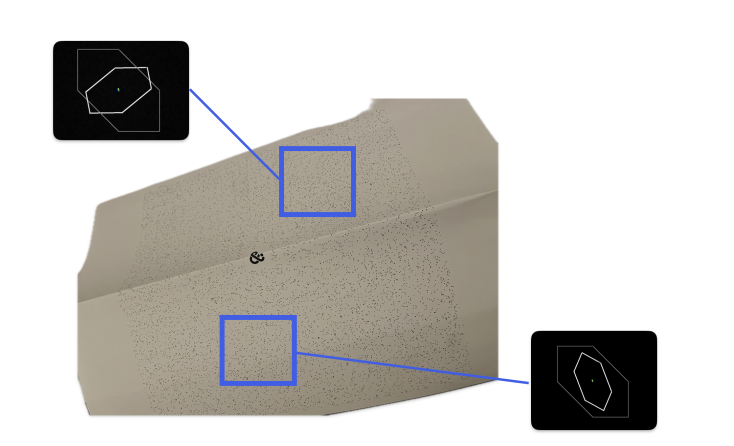
A self-rectifying texture and a QR code printed on paper folded across an edge. The fold makes the QR code unreadable, but the texture reader still recovers the deformation and decodes the tracking information (Bencheikh et al., WACV 2026).

The usual way to undo a perspective distortion is to find distinct points (for example, the three eyes of a QR code) and use their pixel positions to solve for a homography. To stay hidden, self-rectifying textures move the landmarks into the autocorrelation of the image.

Definition of Autocorrelation: The autocorrelation measures how much an image resembles a shifted copy of itself. It is basically a dot product. For a 2D image f:2f: \mathbb{R}^2 \rightarrow \mathbb{R}, the autocorrelation is defined as follows:

Rf,f(τ)=2f(x)f(x+τ)dx R_{f,f}(\tau) = \int_{\mathbb{R}^2} f(x)\, f(x + \tau)\, dx

where xx is a pixel position and the lag (or shift) τ2\tau \in \mathbb{R}^2. A peak is defined as the τ\tau where Rf,f(τ)R_{f,f}(\tau) attains a local maximum. This operation is translation-invariant.

As autocorrelations are computationally expensive (𝒪(N2))(\mathcal{O}(N^2)), we never compute them directly. Instead, we invoke the Wiener-Khinchin theorem, allowing us to compute the autocorrelation in terms of Fourier transforms (\mathcal{F}): R=1(|(f)|2)R = \mathcal{F}^{-1}(|\mathcal{F}(f)|^2) in 𝒪(NlogN)\mathcal{O}(N\log N).

Task 1 – Constructing Textures: We used a grayscale-version of Steamboat Willie with a fronto-parallel view as our base image.

The base image (left) and its autocorrelation plot (right) with unshifted copy τ=0.\tau=0. A plain image with no modifications give one peak at the center corresponding to τ=0\tau=0.

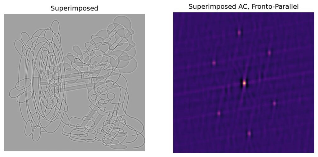
Next, we superimposed three copies of the image, each offset by shift vectors 0,+u,+v20, +u, +v \in \mathbb{R}^2, using zero-padding. We call the superimposed image the base texture. The following autocorrelation plot would have six peaks, at {±u,±v,±(uv)}\{ \pm u, \pm v, \pm (u-v)\} . This is known as the Fundamental Hexagon. Then, we apply a deformation AA to the superimposed image, causing the fundamental hexagon to become {±Au,±Av,±A(uv)}.\{ \pm Au, \pm Av, \pm A(u-v)\}.

The superimposed texture (left) and its six-peak fundamental hexagon (right).
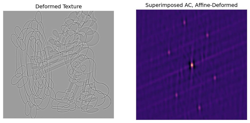
The deformed texture (left) and its warped hexagon (right).

The Assignment Problem: Suppose you know the original shifts {±u,±v,±(uv)}\{ \pm u, \pm v, \pm (u-v)\} and have access to the base texture, but not the deformation. Unfortunately, the deformed hexagon {±Au,±Av,±A(uv)}\{ \pm Au, \pm Av, \pm A(u-v)\} alone does not tell you which peak corresponds to AuAu and which to AvAv, or their signs. However, if you can figure out this assignment problem, then you can immediately solve for AA with some linear algebra.

Given the symmetries, there are eight sign-and-order combinations. Using certain invariance properties, this can be reduced to six combinations. We find and apply six candidate inverse maps A1A^{-1} and select the inverse map with the highest normalized cross-correlation score against the base texture. This is a computationally expensive solution, and for future work, we will explore more efficient methods for the assignment problem.

Task 2 – Full Rectification Pipeline: We introduce a method that no longer assumes a uniform linear deformation. Our goal is to recover a global inverse map ϕ1\phi^{-1} that maps the observed texture back to a fronto-parallel image.
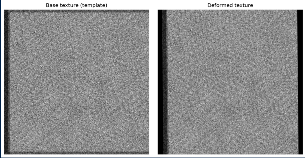
For this experiment, we used blurred Gaussian white noise as our base image, constructing a texture by superimposing it with two shifted copies of itself and zero-padding. We then apply a homography deformation AA.

Methodology: We sample small square patches from the grid. Then, we compute each patch’s autocorrelation and patches with “unreliable measurements” are discarded — criteria include: no valid fundamental hexagon detected or the inverse Jacobian’s determinant is a statistical outlier). For each patch, we detect the warped fundamental hexagon in each patch’s autocorrelation. Comparing these peaks with the known original shifts provides six candidates for the local inverse Jacobian Dϕ1(yi)D\phi^{-1}(y_i).

Then, we construct a Delaunay triangulation mesh of the center points of the remaining patches. Two measurements are treated as neighbors when their centers share an edge in the mesh. To select on candidate Jacobian at each vertex, we assume that the physical deformation varies smoothly, so the correct matrices at neighboring vertices should be similar.

We resolve the candidate ambiguity using Minimum Spanning Tree propagation. First, we use a phase correlation on one patch with the original template to select one initial vertex and its actual local Jacobian Dϕ1(yi)D\phi^{-1}(y_i). Suppose vertex ii has been already assigned the matrix GiG_i^\ast while an adjacent vertex jj remains unassigned. For each of the six candidates at jj, we compute the mismatch

dij(k)=GiGj(k)Fd_{ij}^{(k)} = \| G_i^\ast – G_j^{(k)} \|_F

and take the candidate with the minimum Frobenius norm. All edges from assigned vertices to unassigned vertices are stored in a priority queue, and we iteratively assign matrices to unassigned vertices adjacent to vertices with assignment.
Finally, we use a finite-element method that reconstructs a global inverse map whose gradient best matches the selected local Jacobians:

ϕ^1=arg minψVhΩψ(y)A1(y)Fdy.\hat{\phi}^{-1} = \argmin_{\psi \in V_h} \int_\Omega \| \nabla \psi(y)- A^{-1}(y)\|_F dy.

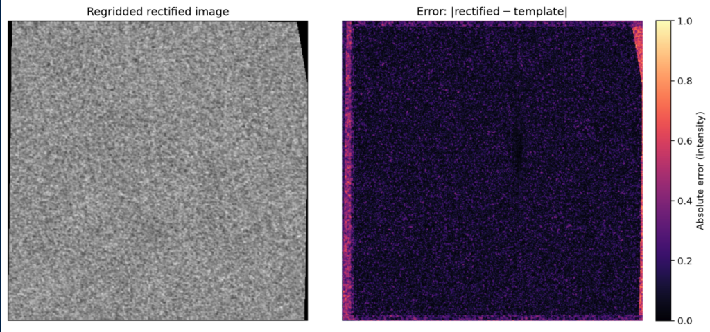
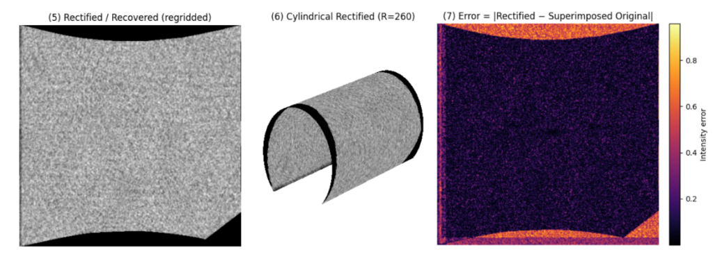
This determines the map up to a constant translation (the +C in integration), so we anchor the reconstructed mesh to the image boundary. We then regrid the deformed pixel values through the recovered map to produce a rectified image. For validation, we compare this result with the original template using the absolute error |rectifiedtemplate||rectified – template|.

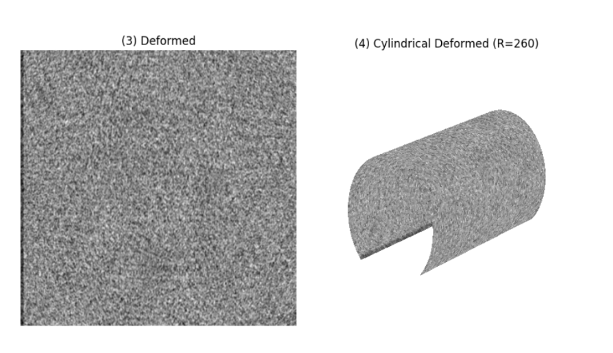
Task 3 – Non-Planar Texture Rectification via Cylindrical Mapping: We extend our rectification pipeline to non-planar surfaces (particularly, a homography-deformed white-noise texture wrapped around a cylinder) utilizing the same MST and Finite Element Method pipeline from Task 2 to recover a global inverse deformation map.

Flattened base texture (left) and cylindrically warped base texture (right).

Note: To model deformations on cylindrical geometry, spatial coordinates (X,Y)(X,Y) in the planar texture domain are mapped to 3D surface coordinates (X,Y,Z)(X,Y, Z) for a cylinder of radius R=260px. To unroll or warp texture fields back into the reference domain, we map the angular coordinates θ=atan2(Y,X)\theta = \text{atan2}(Y,X) back into 2D planar coordinates (X,Y)(X,Y).

Flattened deformed texture (left) and cylindrically warped deformed texture (right)
The resultant unrolled rectified texture (left), cylindrically warped rectified texture (center), and the absolute error against template (right).

Conclusion: Our rectification pipeline has a clear strength: most internal vertices (from the Delaunay triangulation) have sub-pixel error in the rectification and are accurate intensity-wise. However, the pipeline also has two clear weaknesses: (1) there are larger intensity errors at the edges and corners, most likely from our failure to collect as many “good” observations near the edges and corners of the texture and (2) the dependency on accessing the template at least once in the process. Future work would entail resolving these two issues.

References:
[1] Bencheikh, Ismail, et al. “Autocorrelation-based Fiducial Markers for Traceability.” Proceedings of the IEEE/CVF Winter Conference on Applications of Computer Vision. 2026.