Categories
Research

Vortex Loops for Jupiters’ Stripes

Project Members: Aleksa Milovanović, Reid Tang

Mentor: Sadashige Ishida

Introduction to Fluid Dynamics

Fluid motion in computer graphics is typically modeled by the incompressible Navier-Stokes equations:

∂u→∂t+u→⋅∇u→+1ρ∇p=g→+ν∇⋅∇u→,\frac{\partial \vec{u}}{\partial t} + \vec{u} \cdot \nabla \vec{u} + \frac{1}{\rho} \nabla p = \vec{g} + \nu \nabla \cdot \nabla \vec{u},
∇⋅u→=0,\nabla\cdot\vec{u} = 0,

where is the velocity of the fluid, density, pressure, body force and kinematic viscosity. The first equation (momentum) is Newton’s second law applied to fluid elements, and the second one constrains the flow to be volume-preserving.

An important concept is the material derivative, which measures the rate of change of a quantity following a fluid parcel (Lagrangian) rather than at a fixed point in space (Eulerian).

This allows us to write the momentum equation compactly as

Du→Dt+1ρ∇p=g→+ν∇⋅∇u→,\frac{D\vec{u}}{Dt} + \frac{1}{\rho}\nabla p = \vec{g} + \nu\nabla\cdot\nabla\vec{u},

and defines advection s.t. means the quantity is carried by the flow without changing.

Vorticity

Vorticity is defined as the curl of velocity , and measures the local rate of rotation of the fluid. For inviscid flow with no body force, taking the curl of the momentum equation gives the vorticity transport equation

Dω→Dt=(ω→⋅∇)u→\frac{D\vec{\omega}}{Dt} = (\vec{\omega}\cdot\nabla)\vec{u}

where the right-hand side is the vortex-stretching term (as shown in Section 2.1, this term vanishes identically in the 2D setting used throughout this report, so vorticity there is materially conserved exactly, ); it is simply carried by the flow. This makes vorticity important for simulating turbulent and swirl-dominated phenomena, since instead of solving for pressure and velocity everywhere, one only tracks regions where vorticity is concentrated.

The key problem is recovering the velocity field given a vorticity field. In 3D, this is posed as a least-squares problem, i.e. find minimizing

∭‖∇×u→−ω→‖2dV\iiint \|\nabla\times\vec{u} – \vec{\omega}\|^2\,dV

solved via calculus of variations, yielding the Poisson problem , whose solution is the Biot-Savart law:

u→(x→)=∭−∇Φ3(x→−p→)×ω→(p→)dp→,Φ3(x→)=−14π‖x→‖\vec{u}(\vec{x}) = \iiint -\nabla\Phi_3(\vec{x} – \vec{p})\times\vec{\omega}(\vec{p})\,d\vec{p}, \quad \Phi_3(\vec{x}) = -\frac{1}{4\pi\|\vec{x}\|}
Deriving the 2D analogue

Jupiter’s bands and jet streams are a 2D phenomenon (a thin shell on the planet’s surface), so we re-derive the above for a 2D velocity field , where vorticity reduces to a scalar:

ω=∂v∂x−∂u∂y=:curl2(u→)\omega = \frac{\partial v}{\partial x} – \frac{\partial u}{\partial y} =: \mathrm{curl}_2(\vec{u})

In this 2D setting points purely out of the plane while is purely in-plane, so the vortex-stretching term from Section 2 vanishes identically — not as an extra assumption, but automatically, because there is no out-of-plane direction left for vorticity to be stretched or tilted into. The vorticity transport equation therefore simplifies exactly to in 2D, which is what we use throughout.

As in 3D, we seek minimizing

∬(curl2(u→)−ω)2dA\iint \big(\mathrm{curl}_2(\vec{u}) – \omega\big)^2\,dA

Perturbing and using linearity of , the stationarity condition gives, with ,

∬fcurl2(p→)dA=0 , for all p→\iint f\, \mathrm{curl}_2(\vec{p})\,dA = 0 \ \text{, for all } \vec{p}

Unlike 3D, maps a vector field to a scalar, so its adjoint maps a scalar back to a vector. Integrating by parts term by term (boundary terms vanish as fields decay at infinity),

∬fcurl2(p→)dA=∬p→⋅∇⟂fdA,∇⟂f≡(∂f∂y,−∂f∂x)\iint f\,\mathrm{curl}_2(\vec{p})\,dA = \iint \vec{p}\cdot\nabla^\perp f\,dA, \quad \nabla^\perp f \equiv \left(\frac{\partial f}{\partial y},-\frac{\partial f}{\partial x}\right)

so that, since this must vanish for all ,

∇⟂(curl2(u→))=∇⟂ω\nabla^\perp\big(\mathrm{curl}_2(\vec{u})\big) = \nabla^\perp\omega

The same vector identity used in 3D,

∇×∇×u→=−∇⋅∇u→+∇(∇⋅u→)\nabla\times\nabla\times\vec{u} = -\nabla\cdot\nabla\vec{u} + \nabla(\nabla\cdot\vec{u})

restricted to 2D becomes . With the constraint , we obtain a Poisson problem:

−∇⋅∇u→=∇⟂ω-\nabla\cdot\nabla\vec{u} = \nabla^\perp\omega

The 2D fundamental solution of the Laplacian is

Φ2(x→)=12πlog⁡‖x→‖\Phi_2(\vec{x}) = \frac{1}{2\pi}\log\|\vec{x}\|

satisfying , verified by the divergence theorem on the unit circle:

∮∇Φ2⋅n^dℓ=∮12πdℓ=1\oint \nabla\Phi_2\cdot\hat{n}\,d\ell = \oint \frac{1}{2\pi}\,d\ell = 1

The solution to the Poisson problem, via convolution with :

u→(x→)=∬Φ2(x→−p→)∇⟂ω(p→)dp→\vec{u}(\vec{x}) = \iint \Phi_2(\vec{x} – \vec{p})\,\nabla^\perp\omega(\vec{p})\,d\vec{p}

Integrating by parts once again (moving off onto ) gives the 2D Biot-Savart law in the form:

u→(x→)=∬ω(p→)∇⟂Φ2(x→−p→)dp→\vec{u}(\vec{x}) = \iint \omega(\vec{p})\,\nabla^\perp\Phi_2(\vec{x}-\vec{p})\,d\vec{p}

Discretizing as a sum of Dirac deltas collapses the integral to a sum:

u→(x→)=∑iΓi2π(x→−x→i)⟂‖x→−x→i‖2\vec{u}(\vec{x}) = \sum_i \frac{\Gamma_i}{2\pi} \frac{(\vec{x} – \vec{x}_i)^\perp}{\|\vec{x} – \vec{x}_i\|^2}

Since inviscid vorticity is materially conserved, each point vortex simply moves with the velocity induced by all other vortices at its own location (the self-term is excluded), giving the point vortex dynamics equation:

dx→idt=∑j≠iΓj2π‖x→i−x→j‖2(−(yi−yj),xi−xj)\frac{d\vec{x}_i}{dt} = \sum_{j\neq i}\frac{\Gamma_j}{2\pi\|\vec{x}_i-\vec{x}_j\|^2}\big(-(y_i-y_j),\,x_i-x_j\big)

This is the equation we implemented and verified on various examples (e.g. leapfrogging etc.) before extending it to the sphere.

Implementation and Validation in the Plane

The point vortex dynamics equation above was implemented in Houdini using a custom SOP Solver: each timestep, a VEX wrangle reads the previous frame’s point cloud (position and circulation per point), evaluates the Biot–Savart sum, and advances each point’s position. Before trusting this on any nontrivial configuration, it was validated against two exactly-solvable two-vortex cases: equal circulations , where both vortices orbit a common, stationary centroid on a circular path, and opposite circulations , where the pair instead translates together in a straight line at constant speed. Both matched their analytic period/speed formulas.

As a further, qualitative check, a classical four-vortex leapfrogging configuration (two counter-rotating pairs, arranged so the trailing pair periodically overtakes the leading pair) was simulated and reproduced the expected periodic behavior.

Trajectories of the four-vortex leapfrogging configuration at three points in the cycle (frames 20, 80, 140). Each mark traces the recent path of one vortex; the pairs periodically exchange places as they orbit and overtake one another.

A Vortex-Ring Model of Kelvin–Helmholtz Instability

To move from the plane to Jupiter’s spherical atmosphere, the point vortex equation was extended to the unit sphere by replacing the planar kernel with the spherical Biot–Savart law and integrating positions via the exponential map, , so that points remain exactly on the sphere regardless of step size. Because has no boundary, the total vorticity must also integrate to zero, — a constraint with no analogue in the plane, enforced here by construction (equal numbers of positive and negative vortices, or an explicit normalization step subtracting the mean circulation from every point).

On this spherical setup, a shear layer was modeled as a vortex sheet: a ring of point vortices along a line of latitude, one sign on each side of the interface, with a small sinusoidal perturbation added to seed the instability. With no additional forcing, mutual induction alone causes the shear layer to roll up into a periodic array of vortices, as expected from classical vortex-sheet theory.

A single vortex-sheet interface at three stages: the initial perturbed line (frame 50), partial roll-up into discrete billows (frame 250), and a more developed, mixed state (frame 450).

This was then generalized to several alternating-sign rings restricted to a narrower latitude band, approximating Jupiter’s alternating belt/zone structure. Passive marker particles (zero circulation, contributing nothing to the velocity field but advected by it) were added and colored with a Jupiter-like palette for visualization.

Multi-band configuration (M=3) at frames 20, 250, and 500. Marker particles, seeded uniformly, are progressively advected and mixed along the band-induced shear flow.

Modeling the Coriolis Effect

To incorporate planetary rotation, the momentum equation was written in a frame rotating with angular velocity . Taking the curl and combining terms gives the vorticity equation with a rotational source,

DωDt=−2u→⋅Ω→,\frac{D\omega}{Dt} = -2\vec{u}\cdot\vec{\Omega},

in place of the inviscid used above. This was implemented by updating each vortex’s circulation every step, , so that circulation is no longer materially conserved. This is a first, direct discretization of the effect; a more careful treatment (in particular, its interaction with the constraint over long integration times) is left for future work.

Discussion and Limitations

The point-vortex approach reproduces known analytic solutions in the plane, the classical leapfrogging trajectory, and qualitatively correct Kelvin–Helmholtz roll-up on the sphere, both for a single interface and for a multi-band configuration resembling Jupiter’s belts and zones. The Coriolis implementation here is a direct, unrefined discretization rather than a fully validated one, and the multi-band results are qualitative: parameters such as band spacing, perturbation amplitude, and desingularization radius were chosen for a visually clear roll-up rather than calibrated against a specific analytic growth rate or against Jupiter’s actual physical parameters. Extending the integrator beyond forward Euler, and validating the Coriolis term against a known conserved quantity, are the natural next steps.
Categories
Research

Linear Subspace Exploration for Mechanical Systems

Project Members: Al Rahim Hossain, Stephanie Jung, Aleksa Milovanović, Reid Tang

Mentors: Otman Benchekroun, Ty Trusty

Introduction

Simulating deformable objects often requires optimizing over a large number of unknowns. For example, a 2D mesh with nn vertices has 2n2n positional variables: an xx and yy coordinate for each vertex. A 3D mesh similarly has 3n3n positional variables.

In a full order model, the deformed shape is represented by a vector 𝐱\mathbf{x} containing all vertex positions. It is found by minimizing the total energy of the object:

𝐱∗=argmin𝐱(Eelastic(𝐱)+Eext(𝐱))\mathbf{x}^*=\underset{\mathbf{x}}{\text{argmin}}\left(E_{\mathrm{elastic}}(\mathbf{x})+E_{\mathrm{ext}}(\mathbf{x})\right)

where EelasticE_{\mathrm{elastic}} measures how much the object resists being deformed from its rest shape and EextE_{\mathrm{ext}} represents external forces. The solution 𝐱∗\mathbf{x}^* is the state with the lowest total energy, where the elastic response and external forces are balanced. However, this solution may be computationally expensive as it treats every vertex position as an independently moving variable.

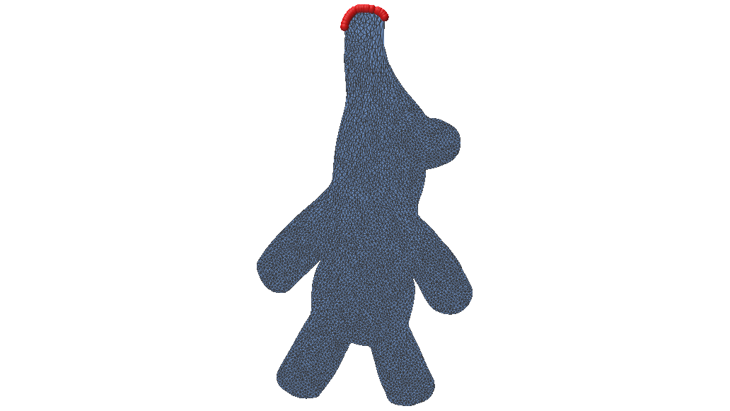
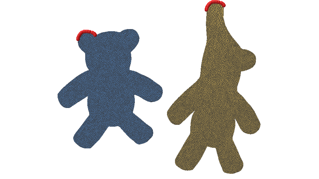
Figure 1: Comparison of the original 2D mesh (left) and its Neo-Hookean deformation (right) under gravity (g=−0.1g = -0.1), with fixed vertices highlighted in red. This represents the exact solution 𝐱∗\mathbf{x}^* found using Newton’s method.

Reduced-Order Model

Reduced-order modelling reduces the size of this optimization by restricting the solution to a low-dimensional subspace. Instead of tracking every point independently, we choose a small set of meaningful deformation patterns. We then approximate the full configuration as 𝐱≈𝐱𝟎+𝐁𝐳\mathbf{x} \approx \mathbf{x_0 + Bz} where 𝐱𝟎\mathbf{x_0} is the rest state of the object, the columns of matrix 𝐁\mathbf{B} represent the selected deformation patterns, and vector 𝐳\mathbf{z} contains their corresponding coefficients [1]. We can now solve for

𝐳∗=argmin 𝐳E(𝐱𝟎+𝐁𝐳)\mathbf{z}^* = \underset{\mathbf{z}}{\text{argmin }}E(\mathbf{x_0 + Bz})

and the final full-space solution is given by 𝐱∗≈𝐱𝟎+𝐁𝐳∗\mathbf{x}^* \approx \mathbf{x_0 + Bz}^*.

The effectiveness of a reduced-order model depends heavily on the choice of the basis 𝐁\mathbf{B}. Ideally, its columns should capture the important deformation patterns of the object using as few modes as possible. There are several ways to construct such a basis.

Proper Orthogonal Decomposition

Proper Orthogonal Decomposition constructs the basis from a dataset of observed or simulated deformations [2]. It finds the directions that best capture the variation present in the example shapes, making it a data-driven approach. It is found by solving

𝐁=argmin 𝐁||𝐗−𝐁𝐁T𝐗||2\mathbf{B} = \underset{\mathbf{B}}{\text{argmin }} ||\mathbf{X – BB}^T\mathbf{X}||^2 such that 𝐁T𝐁=𝐈\mathbf{B}^T\mathbf{B=I}

Here, 𝐗\mathbf{X} is a matrix whose columns contain example displacement vectors from the rest configuration of the object. We use singular value decomposition, 𝐗=𝐔𝐒𝐕T\mathbf{X} = \mathbf{USV}^T, to find the deformation patterns that best represent these examples. The columns of 𝐔\mathbf{U} are ordered from most to least important so if we want a reduced space with 20 modes, for example, we simply take the first 20 columns 𝐁=𝐔[:,:20]\mathbf{B} = \mathbf{U}[:, :20].

Figure 2: Top: Full-order solutions with gravity g∈[−0.002,−0.003,−0.004,−0.005,−0.006,−0.007]g \in [-0.002, -0.003, -0.004, -0.005, -0.006, -0.007] used to form the dataset. Bottom: Deformation under gravity g=−0.1g = -0.1 using POD. Fixed vertices highlighted in red.

A main drawback of POD is that it requires collecting a representative set of deformation examples beforehand. The resulting subspace can only represent deformation patterns present in, or similar to, this training data, so unseen motions may be captured poorly.

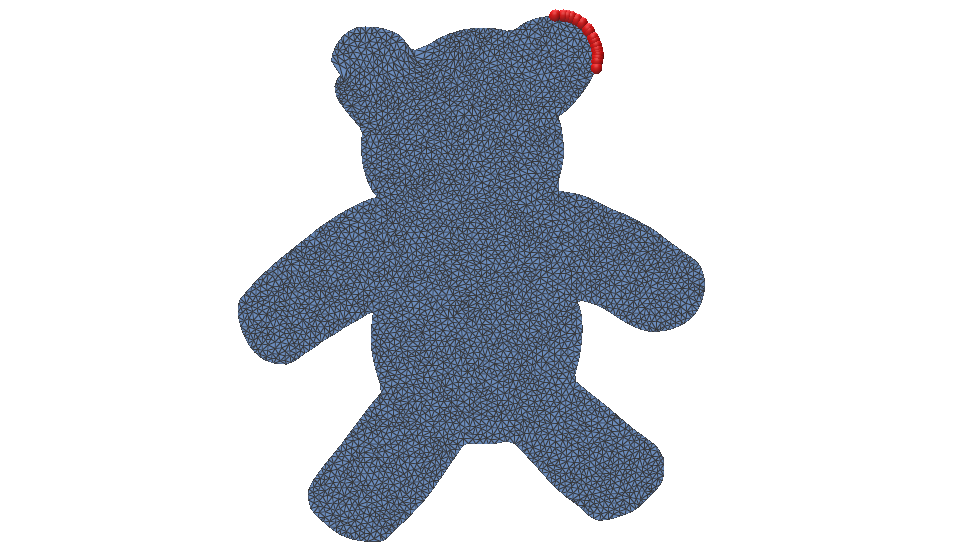
Figure 3: Deformation under gravity g=−0.1g = -0.1 using the POD basis from Figure 2 but with fixed vertices on the opposite ear. It fails since this configuration is not represented in the basis.

Linear Modal Analysis

Linear Modal Analysis builds the reduced basis from the object’s natural vibration modes around its rest shape [3]. The basis vectors are deformation modes obtained from the mesh’s stiffness and mass matrices, so the subspace is determined by the physics of the object rather than by example deformation data. These modes are found by solving the generalized eigenvalue problem

𝐇ϕ=λ𝐌ϕ\mathbf{H}\phi = \lambda\mathbf{M}\phi.

Here, 𝐇\mathbf{H} is the elastic stiffness of the object and 𝐌\mathbf{M} accounts for its mass. Solving the eigenvalue problem gives the natural deformation patterns ϕ\phi, or modes, of the object. The lowest-frequency modes are usually the most important and are chosen as the columns of the reduced basis 𝐁\mathbf{B}.

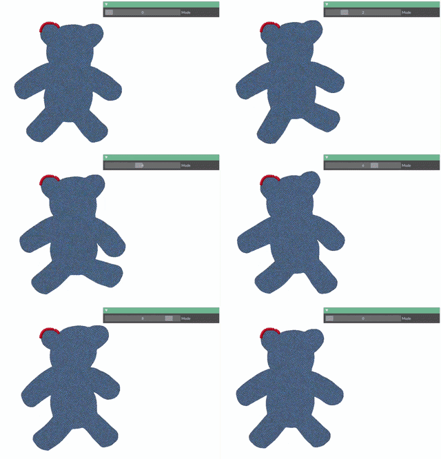
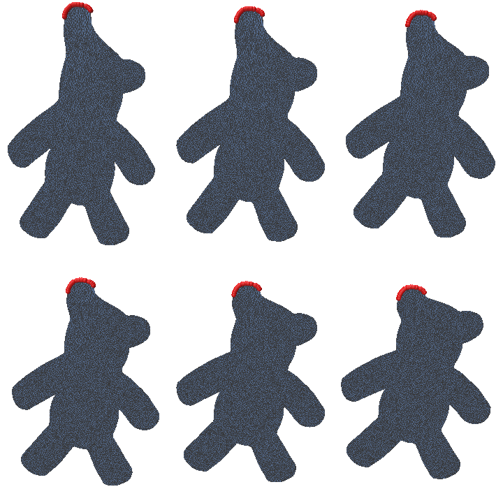
Figure 4: Top: Animation of the first 10 deformation modes. Bottom: Deformation under gravity g=−0.1g = -0.1 using an LMA basis with 5 modes (left), 10 modes (center), and 20 modes (right).

However, LMA is based on a linearization around the rest shape, so it works best for small deformations. Large rotations or strongly nonlinear deformations may not be represented well by a basis of linear vibration modes.

Actuation-Aware Subspaces

POD can capture large deformations, but it requires representative simulation data. LMA avoids this data collection, but its basis is not aware of the parameters driving the simulation. Actuation-aware subspaces build the reduced basis directly from how the object deforms as the actuation parameters change. We write

𝐱(𝐚)=argmin 𝐱E(𝐱,𝐚)\mathbf{x(a)} = \underset{ \mathbf{x} } { \text{argmin } } E(\mathbf{x, a})

where 𝐚\mathbf{a} may represent quantities such as spring rest lengths, gravity, muscle activation, or collider parameters. The goal is to approximate how 𝐱(𝐚)\mathbf{x(a)} changes as 𝐚\mathbf{a} changes.

We can first approximate this relationship using a first-order Taylor expansion around a reference actuation 𝐚0\mathbf{a}_0:

𝐱(𝐚)≈𝐱(𝐚0)+∑i(ai−a0,i)∂𝐱∂ai\mathbf{x}(\mathbf{a})\approx\mathbf{x}(\mathbf{a}_0)+\sum_i(a_i-a_{0,i})\frac{\partial\mathbf{x}}{\partial a_i}.

The derivatives ∂𝐱∂ai\frac{\partial \mathbf{x}}{\partial a_i} describe the deformation caused by changing each actuation parameter. For example, if the object is driven by springs, each parameter could control the rest length of one spring. However, this is still a linear approximation and works best for small deformations near 𝐚0\mathbf{a}_0. Larger motions such as bending, rotation, and compression follow curved deformation paths that cannot be represented well using only fixed linear directions.

To capture these effects, we include second-order derivatives, ∂2𝐱∂ai∂aj\frac{\partial^2 \mathbf{x}} {\partial a_i \partial a_j}, for the second-order Taylor expansion:

𝐱(𝐚)≈𝐱(𝐚0)+∑i(ai−a0,i)∂𝐱∂ai+12∑i∑j(ai−a0,i)(aj−a0,j)∂2𝐱∂ai∂aj\mathbf{x}(\mathbf{a}) \approx \mathbf{x}(\mathbf{a}_0) + \sum_i (a_i-a_{0,i}) \frac{\partial \mathbf{x}}{\partial a_i} + \frac{1}{2} \sum_i\sum_j (a_i-a_{0,i})(a_j-a_{0,j}) \frac{\partial^2 \mathbf{x}}{\partial a_i \partial a_j}

If the first derivatives describe the response to actuation, the second derivatives describe how that response changes as the actuation changes. These terms help capture deformation patterns that appear together during larger motions, allowing the reduced space to follow nonlinear deformation paths more closely.

The reduced subspace can therefore be formed by

𝐁=[∂𝐱∂a1 ⋯ ∂𝐱∂ap ∂2𝐱∂a12 ⋯ ∂2𝐱∂ai∂aj]\mathbf{B} = \left[ \frac{\partial \mathbf{x}}{\partial a_1} \ \cdots\ \frac{\partial \mathbf{x}}{\partial a_p} \ \frac{\partial^2 \mathbf{x}}{\partial a_1^2} \ \cdots\ \frac{\partial^2 \mathbf{x}}{\partial a_i \partial a_j} \right]

such that this space is tailored to the parameters driving the simulation.

This idea is similar to modal derivatives [1], which describe how linear vibration modes change and interact. Here, we apply the same idea to actuation parameters, so the basis is tailored to the forces that will actually drive the simulation.

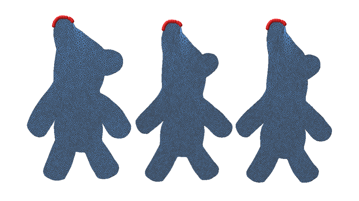
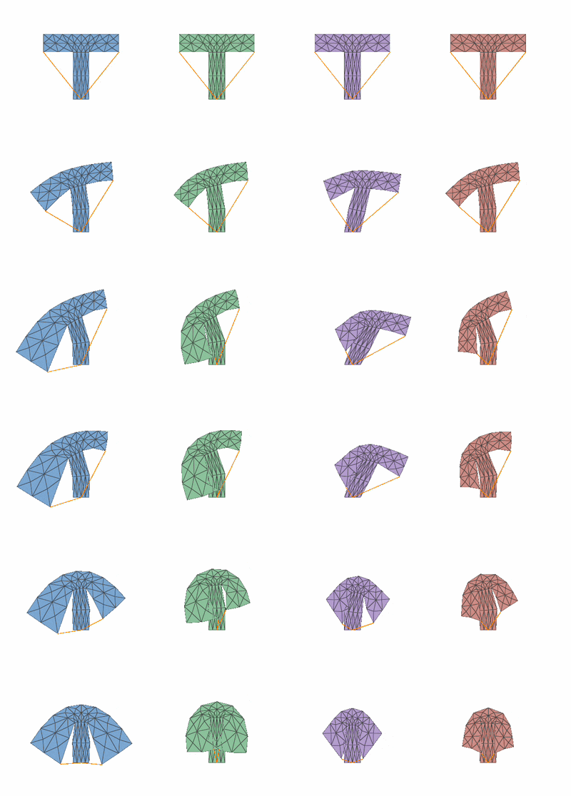
Figure 5: Deformation under spring actuation as the spring is made tighter using (from left to right): first-order approximation, second-order approximation, LMA, and an exact solution using Newton’s method.
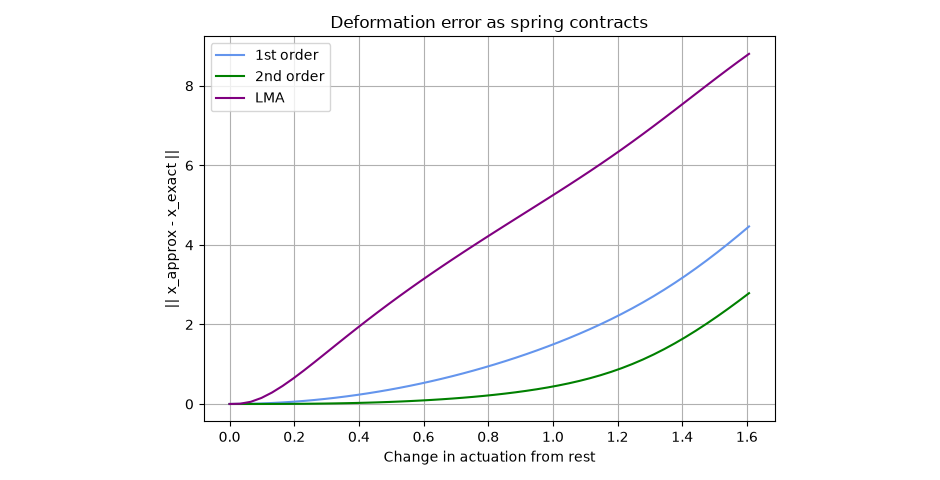
Figure 6: Deformation error as the spring contracts for the first-order, second-order, and LMA reduced models compared with the exact solution.

Conclusion

Reduced-order models can make deformable simulations more efficient by representing motion with a small number of deformation patterns. In this project, we explored an actuation-aware basis that is built from how the equilibrium shape changes with the parameters driving the simulation. First-order derivatives capture the main response to actuation, while second-order derivatives help represent larger and more nonlinear deformations.

There are still several directions for future work. Hyper-reduction is needed to further reduce computational cost [4], and the current method relies on a PSD-projected Hessian for stable basis construction. The number of basis terms also grows with the number of actuation parameters. Future work could address these limitations and extend the method to more complex 3D scenes and different types of actuation.

References

[1] J. Barbič and D. L. James. Real-Time Subspace Integration for St. Venant-Kirchhoff Deformable Models. ACM Transactions on Graphics, 2005.

[2] L. Sirovich. Turbulence and the Dynamics of Coherent Structures. I. Coherent Structures. Quarterly of Applied Mathematics, 45(3), 561–571, 1987.

[3] A. Pentland and J. Williams. Good Vibrations: Modal Dynamics for Graphics and Animation. SIGGRAPH, 1989.

[4] C. Brandt, E. Eisemann, and K. Hildebrandt. Hyper-Reduced Projective Dynamics. ACM Transactions on Graphics, 2018.