by Jayati Sood, Uriel Martínez, Miles Silberling-Cook and Josue Perez
Introduction
The geodesic distance between two points x and y on a mesh is the length of the shortest path from x to y, along the surface. In the first and final weeks of SGI, under the mentorship of Professor Justin Solomon and Professor Nester Guillen, we worked on finding numerical approximations of geodesic distance functions that are low in accuracy and hence faster to compute.
Given a point a set \(S\) of points on the surface \(\mathcal{M}\), we can define a function \(f_S(x):\mathcal{M}\mapsto\mathbb{R}^+\) such that
\[f_S(x) = d(x, S) = \min_{y\in S} d(x,y),\]
where \(d\) is the geodesic distance function in \(\mathcal{M}\). \(f\) satisfies the eikonal equation, i.e.,
\[||\nabla f(x)||_2=1.\]
Solving the eikonal equation with \(f_{S}(x_0)=0\) gives us the geodesic distance function from a given set of points on the mesh/manifold to all other points on the mesh. However, the eikonal equation is a non-linear PDE and hard to solve. To speed up the process, we employ Perron’s method to solve for \(f_{S}(x)\) by finding the maximum of the subsolutions of the above boundary value problem, which leads to the following convex optimization problem:
Our first task was to reformulate this optimization problem for triangle meshes. By restricting paths to the edges of the mesh we arrive at the following. Take our triangle mesh to be an edge-weighted, undirected graph \(G\).
If \(S\subset G\) is the set of vertices to which we are calculating a geodesic, then the distance function \(x\mapsto d(x, S)\) is the unique solution of the following second-order cone program (SOCP):
\[ \begin{align*} \max_f& \;\; \sum \limits_{i=1}^N f(x_i) \\ \text{subject to } & \;\; f(x_i) = 0\;\forall\;x_i\in S \\ & \;\;f(x_i)-f(x_j) \leq \ell_{e} \text{ anytime } e := (x_i,x_j) \in E \end{align*} \]
We can observe from the formulation of the problem that we have two types of constraints. The number of equations we have of the first kind depends directly on the cardinality of \(S\), meanwhile, the number of equations we have of the second type depend on the cardinality of the edges on the mesh. Hence an upper bound on the number of constraints of this particular problem is \(|S|+|E|=\frac{|S|(|S|+1)}{2}\). In other words, the number of constraints in our problem grows quadratically on the amount of vertices on the mesh. Furthermore, there is no good reason why \(f\) should be linear in general, which makes solving this problem even more computationally taxing.
We found that this formulation of the problem (with paths restricted to edges) resulted in poor-quality geodesics with negligible increase in speed. For the remainder of this project we used a form closer to the original, and approximated the gradient with finite differences. Our observations about the number of constraints still apply.
Approach
The approach we took on this project to solve these inconveniences proceeds twofold.
On a first instance, we represent \(f\) in terms of a convenient linear basis, just only for building an approximate notion of distance which takes into account only the elements on the basis that influence the most the values of \(f\), in other words, we build a low resolution geodesic. For selecting this linear base we start calculating the laplacian of the mesh. Then, we select a fixed number of eigenvectors of the matrix, giving preference to those with a lower eigenvalue.
On a second instance, we require the solution of our problem to be of low resolution. We do this by imposing new linear constraints. This could be thought to be contradictory with the goal of the project, however, with the proper use of some standard tools of convex optimization, for example the active set method, in theory we could actually reduce the number of constraints in the original problem. A consequence that we observed by using this approach on reasonably behaved meshes is that the number of active constraints on the problem depends on the size of sampled basis, yielding a method that is almost independent of the cardinallity of \(S\).
Throughout the project, we used cvx in MATLAB to solve our convex program for different sets \(S\) of vertices on the mesh, concluding with \(S\) being the set of all vertices on the mesh, which gave us the distance function for all pairs of vertices. Over the course of the project, we employed various techniques to increase the efficiency of our solver, and were successful in obtaining an all-pairs geodesic distance function on the Spot mesh.
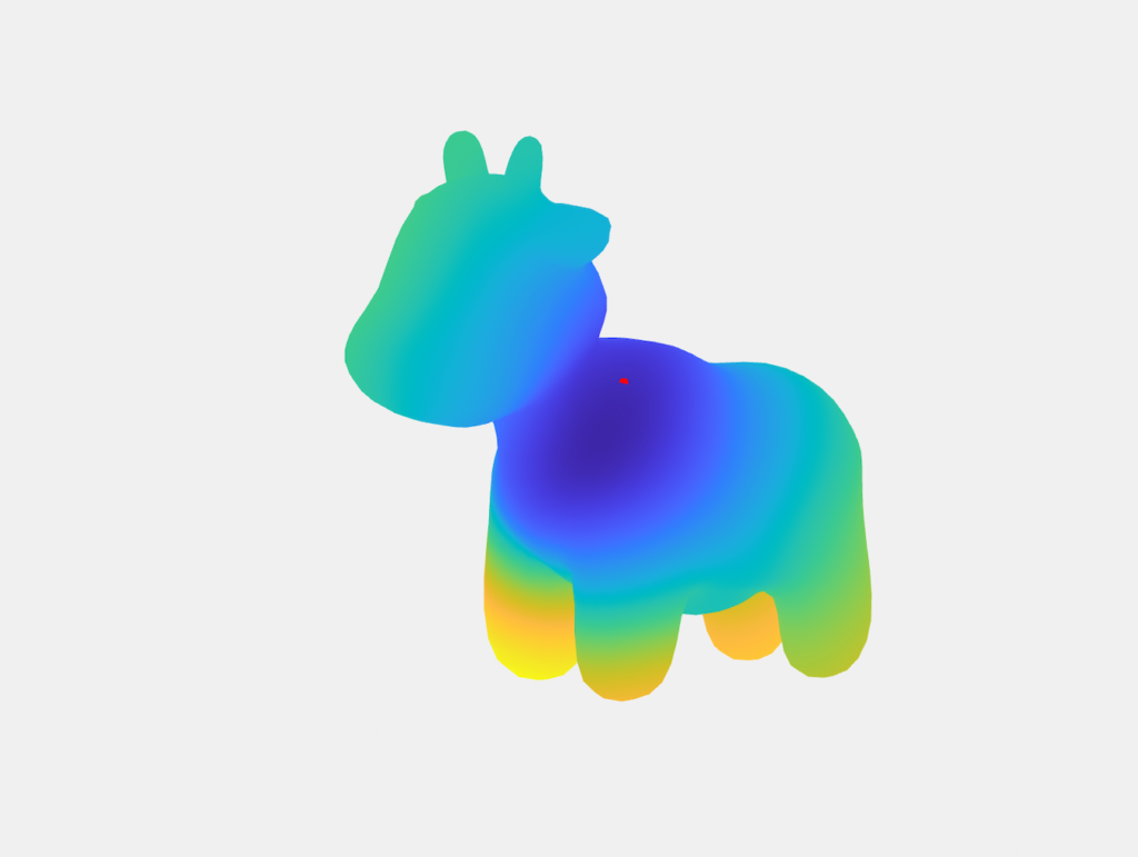
Geodesic distance function heat map
This heat map is a plot of the approximate all-pairs geodesic function for a vertex randomly sampled from Spot. The colour values represent the estimated geodesic distance from the sample vertex (red).
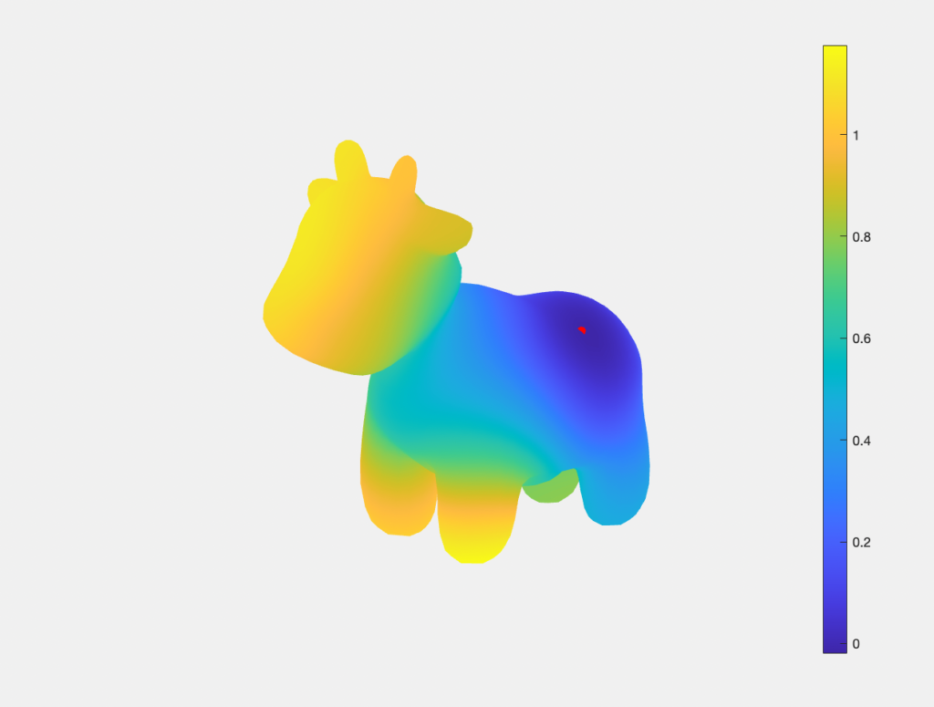
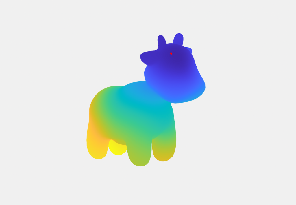
All-pairs geodesic distance function on Spot
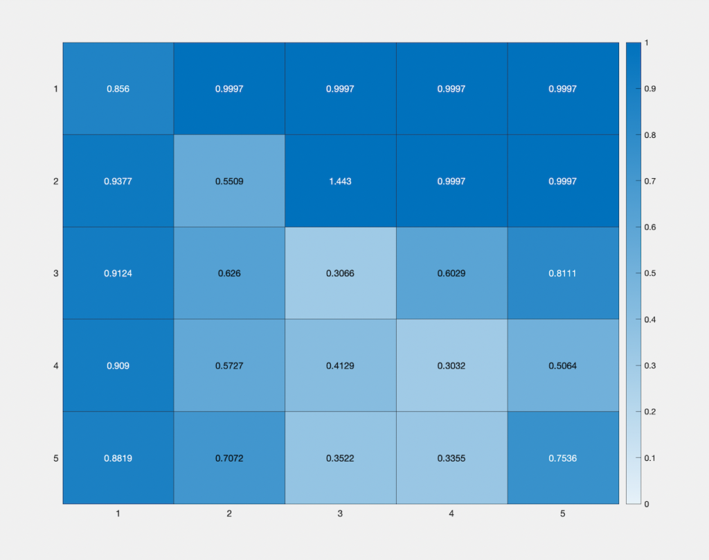
Error map
This heat map represents the change in accuracy of our approximate all-pairs geodesic distance function, with change in the number of basis vectors (vertical), and number of faces sampled (horizontal) from the Spot mesh. The colour values represent the mean relative error between the approximated function and the ground truth geodesic function, with the lightest and darkest blues being assigned to the error values “0” and “1.5”, normalized according to the observed distribution of the error values obtained. Starting with 5 faces and 5 basis vectors, and taking intervals of 5 for both, we observe that the highest accuracy is obtained along the diagonal, i.e, when the number of faces sampled equals the number of basis vectors.
During the third and fourth week of SGI, Xinwen Ding, Ahmed A. A. Elhag and Miles Silberling-Cook (week 3 only) worked under the guidance of Benjamin Jones and Prof. Adriana Schulz to explore methods that can define a continuous relaxation of CAD geometry.
Background
In general, there are two ways to represent shapes: explicit representations and implicit representations. Explicit representations are easier to model and allow local differentiable parameterizations. CAD geometry, stored in an explicit form called parametric boundary representations (B-reps), is one example, while triangle mesh is another typical example.
However, just as each triangle facet in a triangle mesh has its independent parameterization, it is hard to represent a surface using one single function under an explicit representation. We call this property discrete at the global scale. This discreteness forces us to catch continuous changes using discontinuous shape parameterization and results in weirdness and artifacts. For example, explicit representations can be incompatible with some gradient-based methods and some neural network techniques on a non-local scale.
One possible fix to this issue is to use implicit shape representations, such as signed distance field (SDF). SDFs are global functions that are continuously differentiable almost everywhere in the domain, which addresses the issues caused by explicit representations. Motivated by this, we want to play the same trick by defining a continuous relaxation of CAD geometry.
Problem Description
To define this continuous relaxation of CAD geometry, we need to find a continuous relaxation of the boundary element type. Consider a simple case where the CAD data define a geometry that only contains two types; lines and circles. While it is natural that we map lines to 0 and circles to 1, there is no type defined in the CAD geometry as the pre-image of (0,1). So, we want to define these intermediate states between lines and circles.
The task contains two parts. First, we need to learn the SDF and thus obtain the implicit shape representation of the CAD geometry. As an alignment to the input data type, we want to convert the type-blended geometry to CAD data. So next, we want to convert the SDF back to valid boundary representation by recovering the parameters of the elements we encoded in the SDF and then blending their element type.
The Method
To make it easier for the reconstruction task, we decided to learn multiple SDFs, one for each type of geometry. According to these learned SDFs, we can step into the process of recovering the geometries based on their types. Now, let us consider a concrete example. If we have a CAD shape that consists of two types of geometries, say lines and circles, we need to learn two SDFs: one for edges (part of circles) and another for arcs (part of circles). With these learned SDFs, We hope to recover all the lines that appear in the input shape from the line SDF, and a similar expectation applies to the circle SDF.
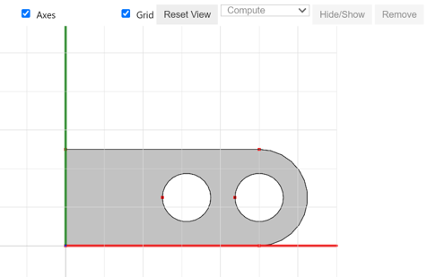
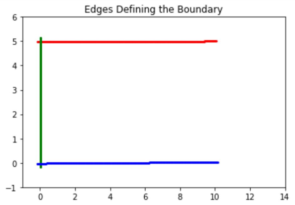
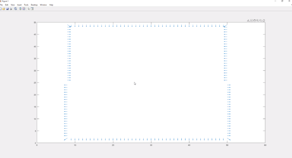
Before jumping into detailed implementations, we want to acknowledge Miles Silberling-Cook for bringing up the multi-SDF idea. Due to the time limitation at SGI, we only tested this method for edges in 2D. We start with the CAD data defining a shape in Figure 1. All the results we show later are based on this geometry.
Figure 1: Input geometry defined by CAD data.
Learned SDF
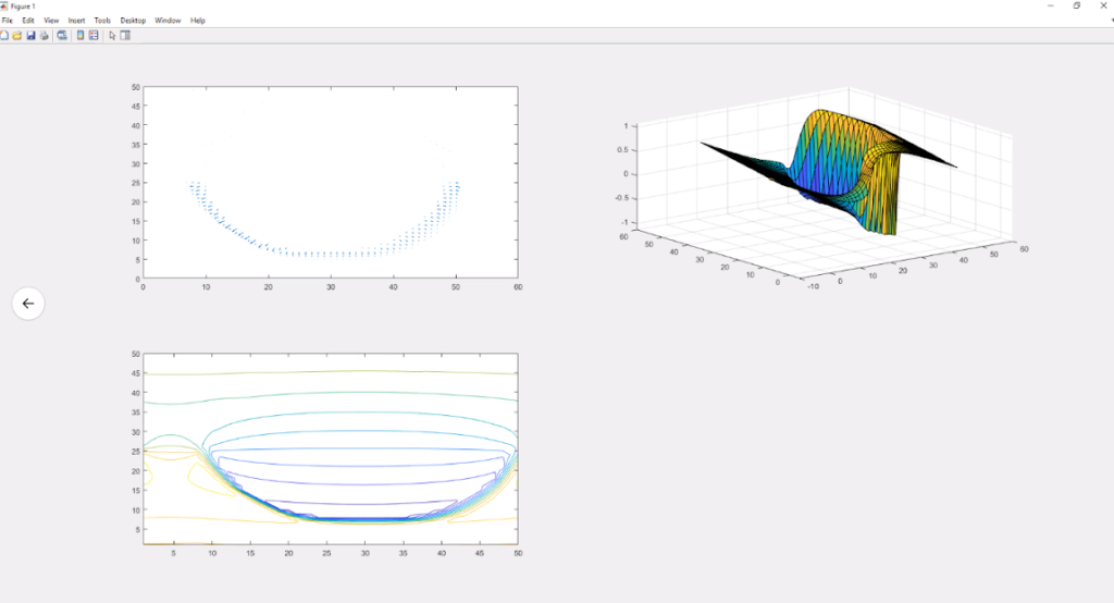
Our goal is to learn a function that maps a coordinate of a query point \((x,y) \in \mathbb{R^2}\) to a signed distance in \(\mathbb{R}\) from \((x,y)\) to the surface. The output of this function is positive if \((x,y)\) is outside the surface, negative if \((x,y)\) is enclosed by the suface, and zero if \((x,y)\) lies on the surface. Thus, our neural network is defined as \(f: \mathbb{R} ^2 \to \mathbb{R}\). For Figure 1, we learned two neural networks, the first network maps \((x,y)\) to its distance from the line edge, and the second network maps this point to its distance for the circle edge. For this task, we use a Decoder network (multi-layer perceptron, MLP), and optimize it using a gradient descent until convergence. Our dataset was created from a grid with appropriate dimensions, as these are our 2D points. Then, for each point in the grid, we calculate its distance from the line edge and the circle edge.
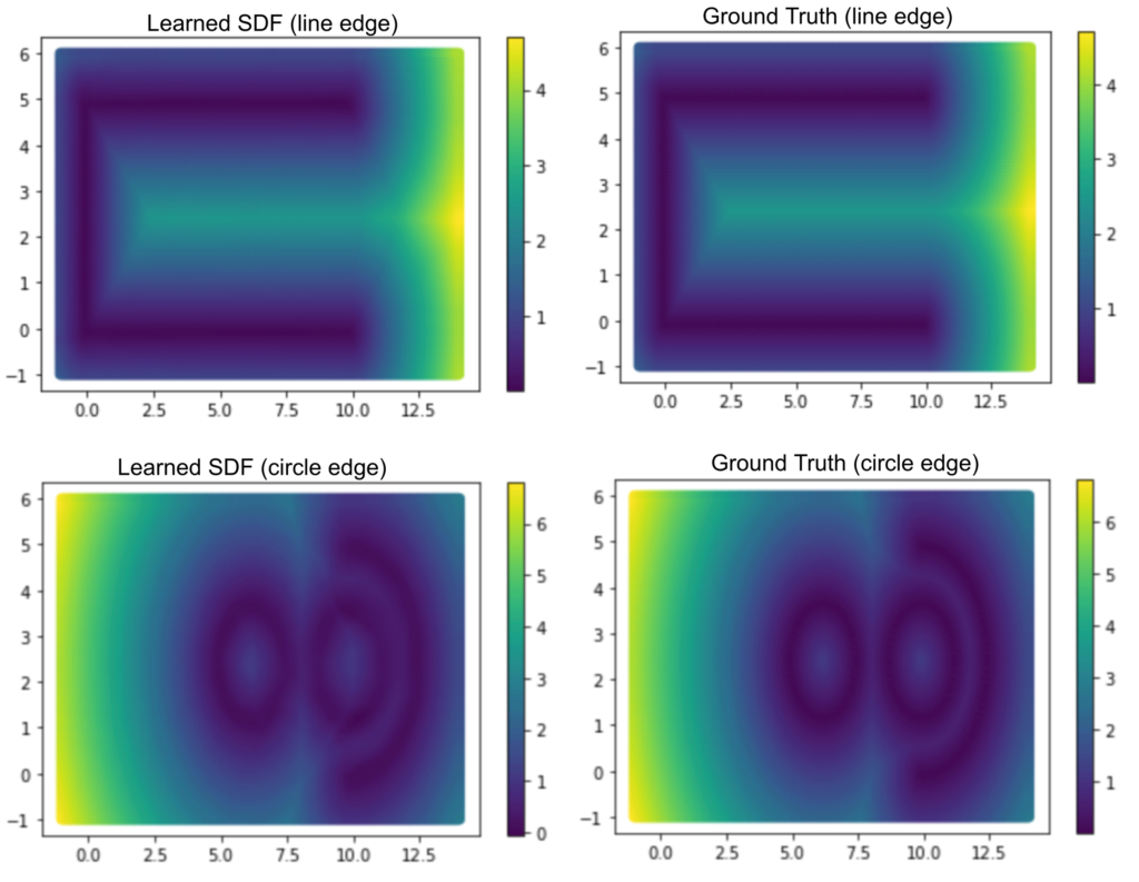
We compare the image from the learned SDF and the ground truth in Figure 2. It clearly shows that we can overfit and learn both the two networks for line and circle edges.
Figure 2: The network learned the SDF with respect to the edges (first row) and arcs (second row) of the input geometry displayed in Figure 1. We compare the learned result (left column) with the ground truth (right column).
Reconstruction
After obtaining the learned line SDF model, we need to analytically recover the edges and arcs. To define an edge, we need nothing but a starting point, a direction, and a length. So, we begin the recovery by randomly seeding thousands of points and assigning each point a random direction. Furthermore, we can only accept those points with their associated values in SDF to be close to zero (see Figure 3), which enhances the success rate of finding an edge as a part of the shape boundary.
Figure 3: we iteratively generate points until 6000 of them are accepted (i.e. SDF value small enough). The accepted points are plotted in red.
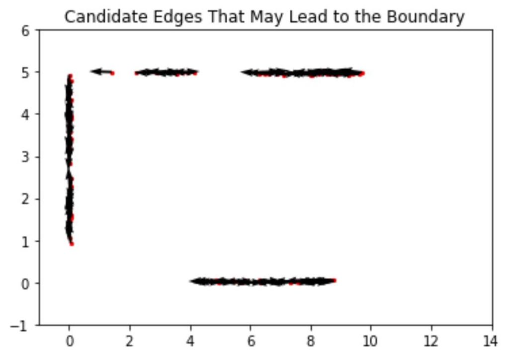
Then, we need to tell which lines are more likely to be the ones that define the boundary of our CAD shape and reject the ones that are unlikely to be on the boundary. To guarantee a fair selection, we need to fix the length of the randomly generated edges and pick the ones whose line integral of the learned line SDF is small enough. Moreover, to save more time, we approximate the integral by a finite sum, where we sum up the SDF value assumed by a fixed number of sample points along every edge. Stopping here, we have a pool of edge boundary candidates. We visualize them in terms of their starting points and direction using a quiver plot in Figure 4.
Figure 4: Starting points (red dots) and proper directions (black arrows) that define potential edges.
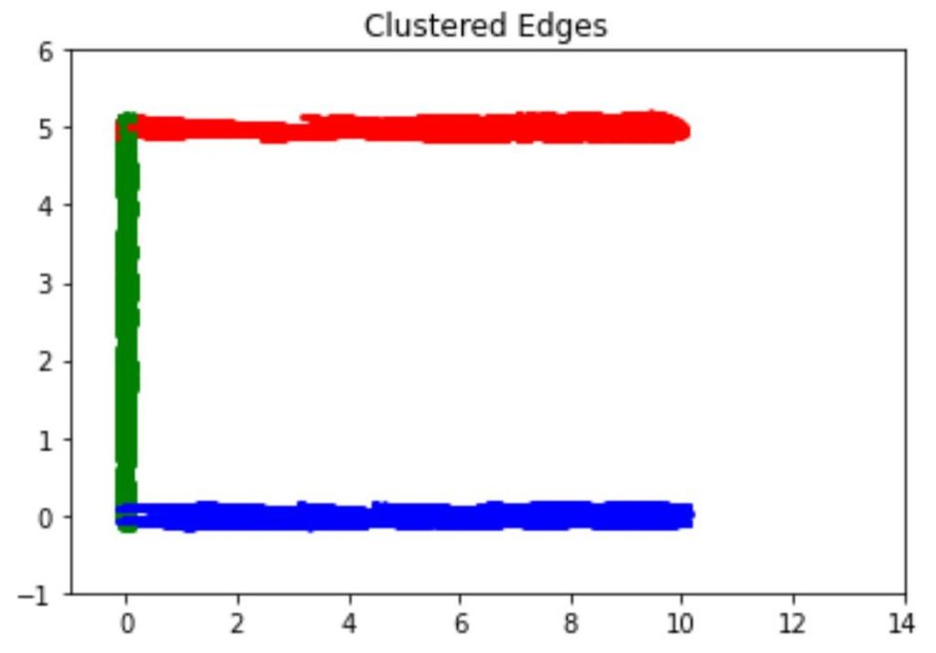
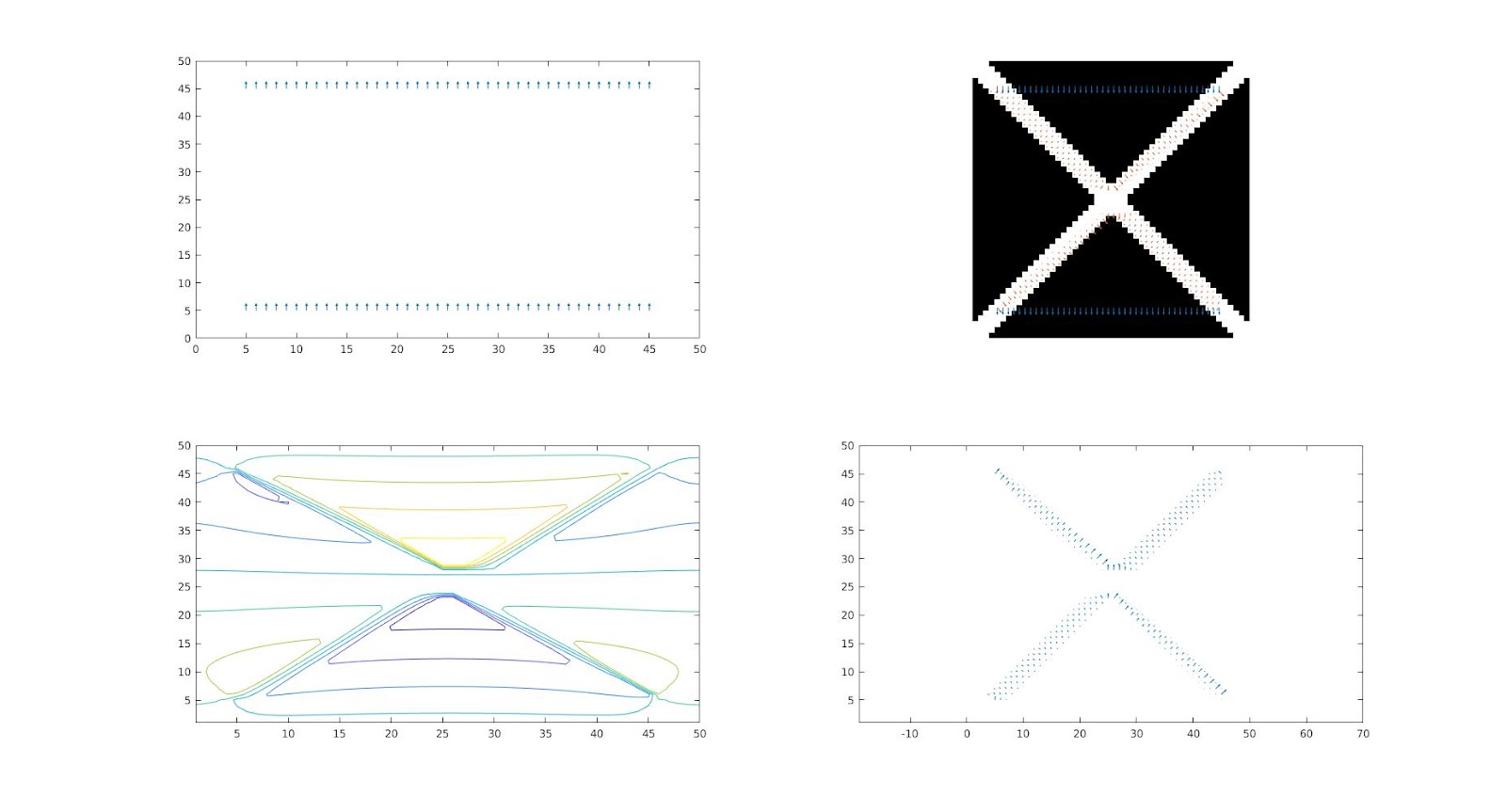
In the next step, we want to extend the candidate edges as long as possible, as our goal is to reconstruct the whole boundary. The extension ends once the SDF value of some extended point exceeds some threshold. After the extension, we cluster the extended edges using the mean shift algorithm. We adopt this clustering algorithm since it does not need to pre-determine the number of clusters. As shown in Figure 5, the algorithm successfully predicts the correct number of edge clusters after carefully tuning the parameters.
Figure 5: Clustered edges. Each color represents one cluster. After carefully tuning parameters, the optimal number of clusters found by the mean shift algorithm reflects the actual number of edges in the geometry.
Finally, we want to extract the lines that best define the shape boundary. As we set a threshold in the extension process, we simply need to choose the longest edge from each cluster and name it a boundary edge. The three boundary edges in our example, one in each color, appear in Figure 6.
Figure 6: The longest edges, one from each cluster, with parameters known.
Results
To sum up, during the project’s two-week active period, we managed to complete the following items:
We set up a neural network to learn multiple SDFs. The model learns the SDF for edge and arc components on the boundary of a 2D input shape.
We developed and implemented a sequence of procedures to reconstruct the lines from the trained line SDF model.
Future Work
Even though we showed the results we achieved during the two weeks, there are more things to improve in the future. First of all, we need to reconstruct the arcs in 2D and ensure the whole procedure to be successful in more complicated 2D geometries. Second, we would like to generalize the whole process to 3D. More importantly, we are interested in establishing a way to smoothly and continuously characterize the shape transfer after the reconstruction. Finally, we need to transfer the continuous shape representation back to a CAD geometry.
by Hector Chahuara, Anna Krokhine and Elshadai Tegegn
Introduction
Controlling caustics is a difficult task as any change to specular surface can have large effects on the caustic image. In this post, we address a building block of the optimization framework for computing the shape of refractive objects presented in Schwartzburg et al (2014) and propose to improve a building block on its formulation that performs a mesh reconstruction. The proposed improvement was tested on flatland meshes and performs reasonably well in the presence of noise.
Theory
Regularization is a technique often needed in optimization for enforcing certain characteristics such as sparsity or stability in the solution. In this particular case, Schwartzburg et al (2014) apply a generalized Tikhonov regularization to achieve a stable solution. Given the optimization-based formulation of Schwartzburg et al (2014), it is possible to isolate this problem and to see that this is in fact mesh denoising. In addition, it is important to mention that Tikhonov regularization is usually outperformed by other methods, among which total variation (TV) denoising distinguishes itself by its reasonable computational cost and good results.
In the following, we apply the framework described in Zhang et al (2015) that applies TV to the noisy normalized normals N0 of a mesh, then the optimization problem to solve becomes
minN ||N-N0||2 + λ.WVTV(N),
where WVTV is a weighted vectorial TV version, adapted from the one described in Zhang et al (2015) for flatland, defined as
WVTV(N) = Σeωe (le(DxN)2+(DyN)2)0.5
le is the length of the edge “e”, and the weights ωe , dependent on the difference of two consecutive normals Ni and Ni+1 i.e. normals that correspond to adjacent edges are defined as
ωe=exp(-||Ni-Ni+1||4)
to penalize less sharp features (high difference between consecutive normals) than the smooth ones (similar consecutive normals). It is important to mention that TV denoising is a non-smooth optimization problem, so a solver that rely solely on gradient or Hessian information could not reach the optimum. By using the iteratively reweighted least squares (IRLS) Wolke et al (1988), a well-known method for optimization, it is straightforward to build an algorithmto solve this problem .
Results
The described approach was implemented in MATLAB R2021b. Visual results can be observed in the following animations that show the denoising process of two figures corrupted by noise: a square and a circle.
Denosing procedure of a square meshDenoising procesdure of a circle mesh
Conclusion
The implemented method yields reasonable results for the presented cases. While this exploratory experiments indicate that the method has the potential to improve results if embedded in the general caustics framework. Nonetheless, more experiments are needed to confirm this and to assess the impact on the quality of the result.
References
Y. Schwartzburg, R. Testuz, A. Tagliasacchi, and M. Pauly, “High-contrast computational caustic design, “ ACM Trans. Graph. 33, 4, 2014
H. Zhang, C. Wu, J. Zhang and J. Deng, “Variational Mesh Denoising Using Total Variation and Piecewise Constant Function Space,” in IEEE Transactions on Visualization and Computer Graphics, vol. 21, no. 7, pp. 873-886, 1 July 2015
Wolke, R., Schwetlick, H., “Iteratively Reweighted Least Squares: Algorithms, Convergence Analysis, “ and Numerical Comparisons. SIAM Journal on Scientific and Statistical Computing, 9, 907-921, 1988
L. Condat, “Discrete total variation: New definition and minimization,” SIAM Journal on Imaging Sciences, vol. 10, no. 3, pp. 1258-1290, 2017
A theoretical walkthrough INRs methods for unoriented point clouds
By Alisia Lupidi, Ahmed Elhag and Krishnendu Kar
Hello SGI Community, 👋 We are the Implicit Neural Representation (INR) team, Alisia Lupidi, Ahmed Elhag, and Krishnendu Kar, under the supervision of Dr. Dena Bazazian and Shaimaa Monem Abdelhafez. In this article, we would like to introduce you to the theoretical background for our project. We based our work on two papers: one about Sinusoidal Representation Network (SIREN[1] ) and one about Divergence Guided Shape Implicit Neural Representation for unoriented point clouds (DiGS[2]), but before presenting these we added a (simple and straightforward) prerequisites section where you can find all the theoretical background needed to understand the papers. Enjoy!
0.Prerequisites
0.1 Implicit Neural Representation (INR)
Various paradigms have been used to represent a 3D object predicted by neural networks – including voxels, point clouds, and meshes. All of these methods are discrete and therefore pose several limitations – for instance, they require a lot of memory which limits the resolution of the 3D object predicted.
The concept of implicit neural representation (INR) for 3D representation has recently been introduced and uses a signed distance function (SDF) to represent 3D objects implicitly. It is a type of regression problem and consists of encoding a continuous differential signal within a neural network. With INR, we can provide a high resolution for a 3D object with a lower memory footprint, despite the limitations of discrete methods.
0.2 Signed Distance Function (SDF)
The signed distance function[5] of a set in Ω is a metric space that determines the distance of a given point 𝓍 from the boundary of Ω. The function has positive values for ∀𝓍 ∈ Ω, and this value decreases as 𝓍 approaches the boundary of Ω. On the boundary, the signed distance function is exactly 0 and it takes negative values outside of Ω.
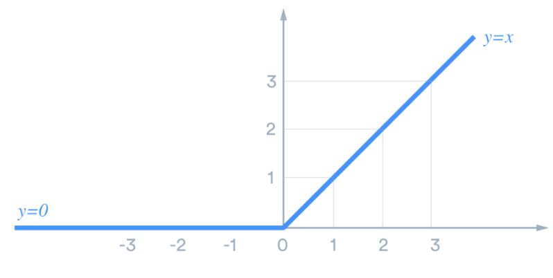
0.3Rectified Linear Unit (ReLU)
The Rectified Linear Unit (ReLU, Fig. 1) is the most commonly used activation function in deep learning models. The function returns 0 if it receives any negative input, but for any positive value 𝓍, it returns that value. It is defined by f(𝓍) = max(0, 𝓍), where 𝓍 is an input to a neuron.
Figure 1: ReLU Plot[3]
ReLU pros
ReLU cons
Extremely easy to implement (just a max function), unlike the Tanh and the Sigmoid activation functions that require exponential calculation
Dying ReLU: for all negative inputs, ReLU gives 0 as output – a ReLU neuron is “dead” if it is stuck in the negative side (not recoverable).
The rectifier function behaves like a linear activation function
A perceptron is a linear classifier that takes in input 𝓎 = ∑ Wᵢ𝓍ᵢ + bᵢwhere 𝓍 is the feature vector, W are the weights, and b the bias. This input, in some cases such as SIREN, is passed to an activation function to produce the bias (see equation 5).
1.SIREN
1.1 Sinusoidal Representation Network (SIREN)
SIRENs[1] are neural networks (NNs) used for signals’ INRs. In comparison with other networks’ architectures, SIRENs can represent a signal’s spatial and temporal derivatives, thus conveying a greater level of detail when modeling a signal, thanks to their sine-based activation function.
1.2 How does SIREN work?
We want to learn a function Φ that satisfies the following equation and is limited by a set of constraints[1],
This above is the formulation of an implicit neural representation where F is our NN architecture and it takes as input the spatio-temporal coordinates 𝓍 ∈ ℝm and the derivatives of Φ with respect to 𝓍. This feasibility problem can be summarized as[1],
As we want to learn Φ, it makes sense to cast this problem in a loss function to see how well we accomplish our goal. This loss function penalizes deviations from the constraints on their domain Ωm[1],
Here we have the indicator function1Ωm= 1 if 𝓍 ∈ Ωmand otherwise equal to 0.
All points 𝓍ᵢ are mapped to Φ(𝓍) in a way that minimizes its deviation from the sampled value of the constraint aᵢ(𝓍). The dataset D = {(𝓍ᵢ, aᵢ(𝓍))}ᵢ is sampled dynamically at training time using Monte Carlo integration. The aim of doing this is to improve the approximation of the loss L as the number of samples grows.
To calculate Φ, we use θ parameters and solve the resulting optimization problem using gradient descent.[1]
Here θi ∶ ℝ→ ℝNiis the ith layer of the network. It consists of the affine transform defined by the weight matrix Wi∈ ℝNix Mi and the biases bi∈ ℝNi applied on the input 𝓍ᵢ∈ ℝMi. The sine acts as the activation function and it was chosen to achieve greater resolution: a sine activation function ensures that all derivatives are never null regardless of their order (the sine’s derivative is a cosine, whereas a polynomial one would approach zero in a number of derivations related to its grade). A polynomial would thus lose higher order frequencies and therefore render a model with less information.
1.3 Examples and Experiments
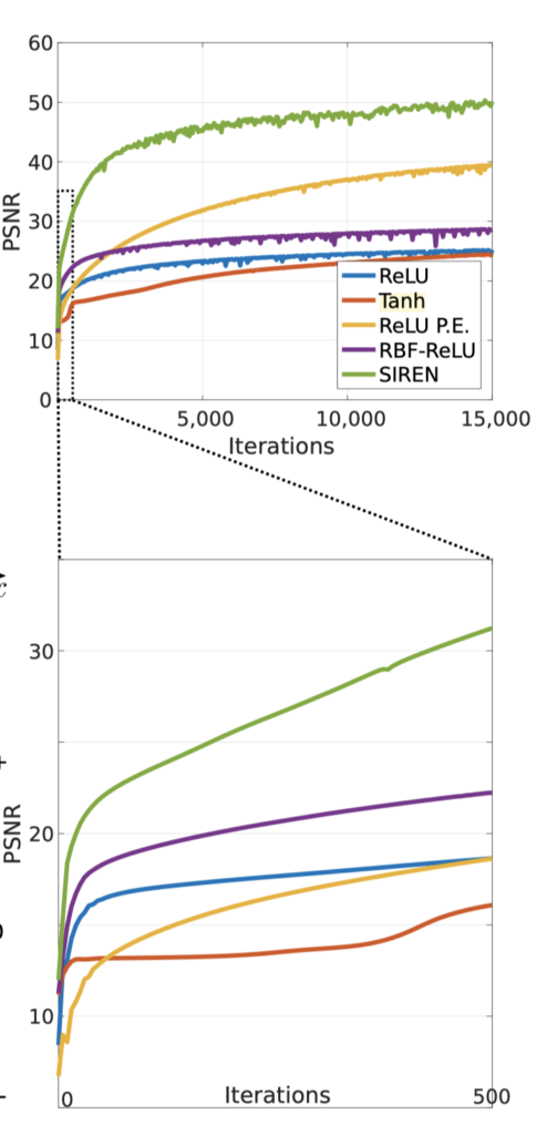
In the paper[1], the authors compared SIREN performances to the most popular network architectures used-like Tanh, ReLU, Softplus, etc. Conducting experiments on different signals (picture, sound, video, etc), we can see that SIREN outperforms all the other methods by a significant margin (i.e., it reconstructs the signal with higher accuracy, Fig. 2).
Figure 2: SIREN performance compared to other INRs.[1]
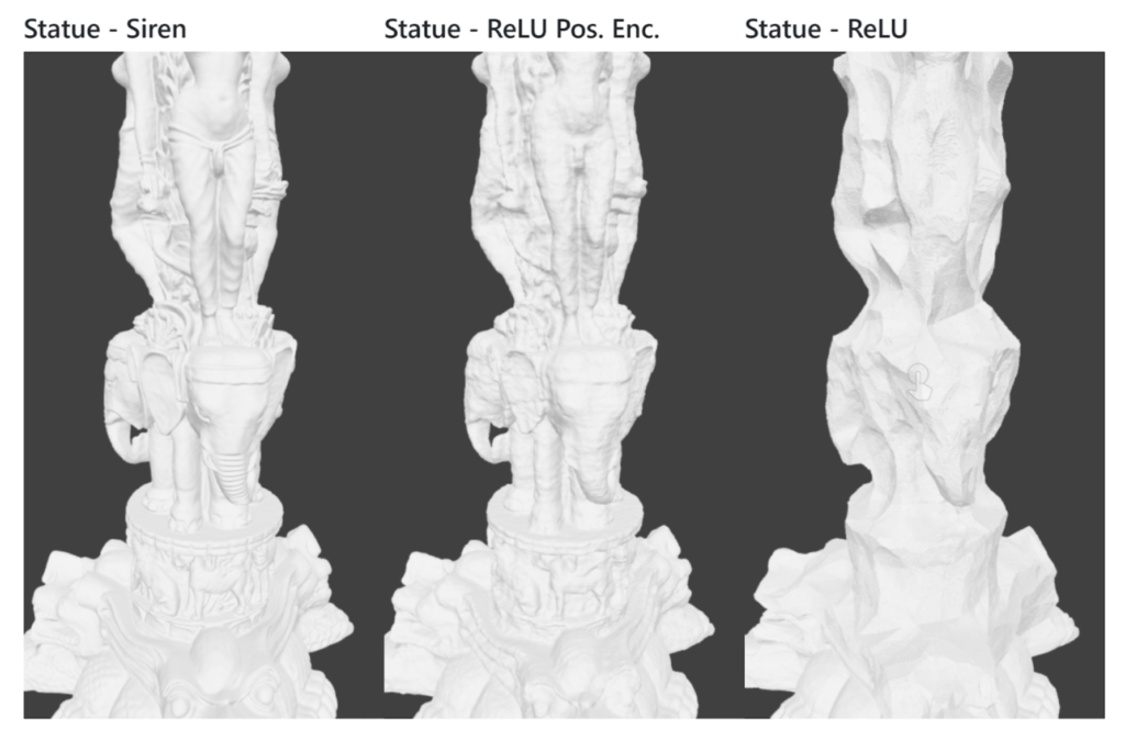
To appreciate all of SIREN’s potential, it is worth mentioning that we can look at the experiment the authors did on an oriented point cloud representing a 3D statue and on shape representation with differentiable signed distance functions (Fig. 3).
Figure 3: SIREN reconstruction of a high detailed statue compared to ReLU ones.[5]
By applying SIREN to this problem, they were able to reconstruct the whole object while accurately reproducing even the finer details on the elephant and woman’s bodies.
The whole scene is stored in the weights of a single 5-layer NN. Compared to recent procedures (like combining voxel grids with neural implicit representations) with SIREN, we have no 2D or 3D convolutions and fewer parameters.
What gives SIREN an edge over other architectures is that: it does not compute SDFs using supervised GT SDF or occupancy values. Instead, it requires supervision in the gradient domain, so even though it is a harder problem to solve, it results in a better model and more efficient approach.
1.4 Conclusion on SIREN
SIREN is a new and powerful method in the INR world that allows 3D image reconstructions with greater precision, an increased amount of details, and smaller memory usage. All of this has been possible thanks to a smart choice of the activation function: using the sine gives an edge on the other networks (Tanh, ReLU, Sigmoid, etc) as its derivatives are never null and retrieve information even at higher frequency levels (higher order derivatives).
2.DiGS
2.1Divergence Guided Shape Implicit Neural Representation for unoriented point clouds (DiGS)
Now that we know what SIREN is, we present DiGS[2]: a method to reconstruct surfaces from point clouds that have no normals.
Why are normals important for INR? When normal vectors are available for each point in the cloud, a higher fidelity representation can be learned. Unfortunately, most of the time normals are not provided with the raw data. DiGS is significant because it manages to render objects with high accuracy in all cases, thus bypassing the need for normals as a prior.
2.2Training SIRENs without normal vectors
The problem has now changed into training a SIREN without supplying the shape’s normals beforehand.
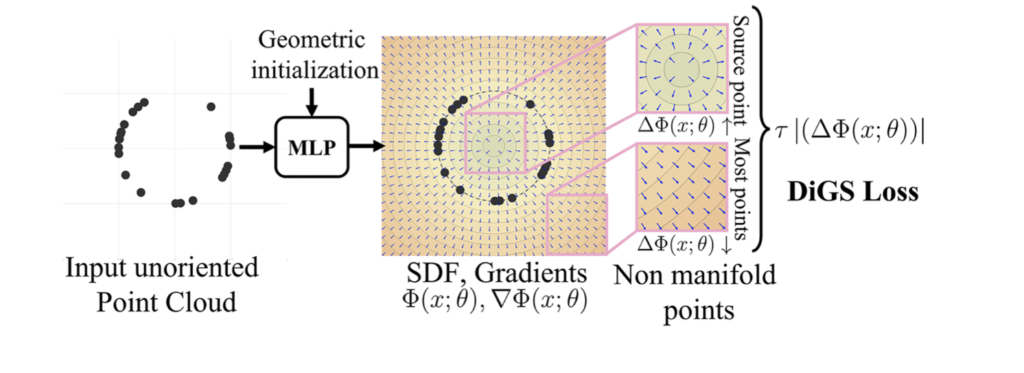
Looking at the gradient vector field of the signed distance function produced by the network, we can see that it has low divergence nearly everywhere except for sink points – like in the center of the circle in Fig. 4. By incorporating this geometric prior as a soft constraint in the loss function, DiGS reliably orients gradients to match the unknown normals at each point and in some cases this produces results that are even better than those produced by approaches that use directly GT normals.
Figure 4: DiGS applied to a 2D example. [2]
To do this, DiGS requires a network architecture that has continuous second derivatives, such as SIRENs, and an initial zero level set that is approximately spherical. To achieve the latter, two new geometric initialization methods are proposed: the initialization to a sphere and the Multi-Frequency Geometric Initialization (MFGI). The MFGI is better than the first because the first keeps all activations within the first period of the sinusoidal activation function and this will not generate high-frequency outputs, thus losing some detail. The second one, however, introduced controlled high frequencies into the first layer of the NN, and even though is a noisier method it solves the aforementioned problem.
To train SIRENS with DiGS, firstly we need a precise geometric initialization. Initializing the shape to a sphere biases the function to start with an SDF that is positive away from the object and negative in the center of the object’s bounding box, while keeping the model’s ability to have high frequencies (in a controllable manner). Progressively, finer and finer details are added into consideration, passing from a smooth surface to a coarse shape with edges. This step-by-step approach allows the model to learn a function that has smoothly changing normals and that is interpolated as much as possible with the original point cloud samples.
The original SIREN loss function includes:
A manifold constraint: points on the surface manifold should be on the function’s zero-level set[2],
A non-manifold penalization constraint because of which all off-surface point have SDF = 0[2],
An Eikonal term that defines all gradients to have unit length[2],
A normal term that forces the gradients’ directions of points on the surface manifold to match the GT normals’ directions[2],
The original SIREN’s loss function is[2]
With DiGS, the normal term is replaced by a Laplacian one that imposes a penalty on the magnitude of the divergence of the gradient vector field.[2]
This leads to a new loss function which is equivalent to regularizing the learn loss function:[2]
2.3 Examples and Experiments
Iterations
0
50
2000
9000
DiGS
SIREN
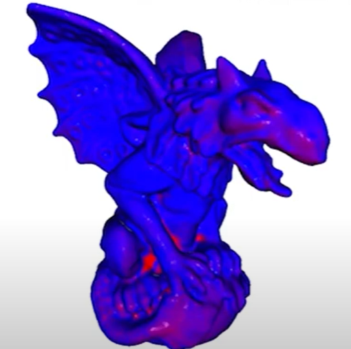
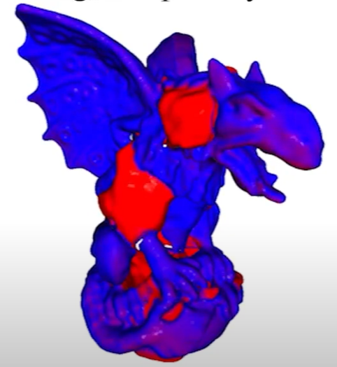
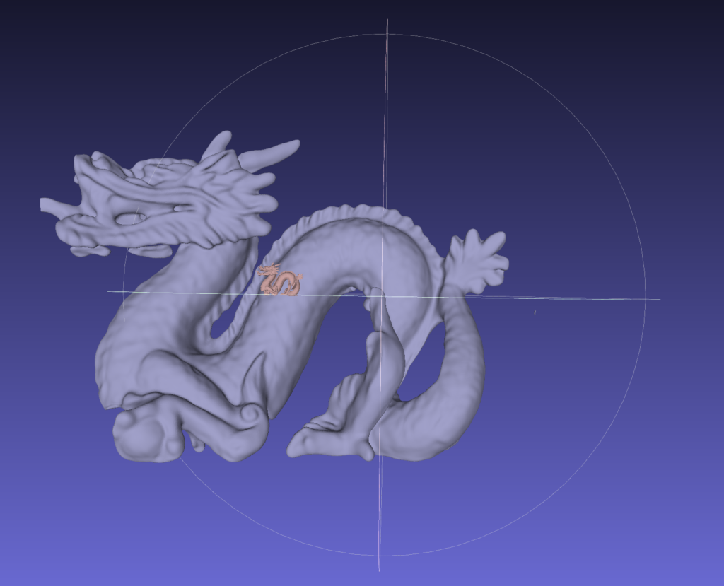
Figure 5: Reconstructing a dragon statue (DIGS and SIREN).[7]
In Fig. 5, both SIREN and DiGS were tasked with the reconstruction of a highly detailed statue of a dragon for which no normals were provided. The outputs were color mapped: in red, you can see the approximated solution, and in blue the reconstructed points match exactly with the ground truth.
At iteration 0, we can appreciate the spherical geometrical initialization required by DiGS. At first, it seems that SIREN converges faster and better to the solution: after 50 iterations, in fact, SIREN already has the shape of the dragon whereas DiGS has a potato-like object. But as the reconstruction progresses, SIREN gets stuck on certain areas and cannot derive them. This phenomenon is known as “ghost geometries” (see Fig 6) as no matter how many iterations we do INR architectures cannot reconstruct these areas. This means that our results will always have irrecuperable holes. DiGS is slower but can overcome ghost geometries: after 9k iterations, DiGS manages to recover data for the whole statue – irrecuperable areas included.
Figure 6: Highlighting ghost geometries. [7]
2.4 Conclusion on DiGS
In general, DiGS behaves as good as (if not better) than other state-of-the-art methods with normal supervision and can also overcome ghost geometries and deal with unoriented point clouds.
3. Conclusions
Being able to reconstruct shapes from unoriented point clouds expands our ability to deal with incomplete data, which is something that often occurs in real life. As point clouds dataset without normals is more common than those with normals, the advancements championed by SIREN and DiGS will greatly facilitate 3D model reconstruction.
Acknowledgements
We want to thank our supervisor Dr. Dena Bazazian, and our TA Shaimaa Moner, for guiding us through this article. We also want to thank Dr. Ben-Shabat for his kindness in answering all our questions about his paper.
References
[1] Sitzmann, V., Martel, J., Bergman, A., Lindell, D. and Wetzstein, G., 2020. Implicit neural representations with periodic activation functions. Advances in Neural Information Processing Systems, 33, pp.7462-7473.
[2] Ben-Shabat, Y., Koneputugodage, C.H. and Gould, S., 2022. DiGS: Divergence guided shape implicit neural representation for unoriented point clouds. In Proceedings of the IEEE/CVF Conference on Computer Vision and Pattern Recognition, pp. 19323-19332.
[4] Sitzmann, V., 2020, Implicit Neural Representations with Periodic Activation Functions [online], https://www.vincentsitzmann.com/siren/, [Accessed 27 July 2022].
[5] Chan, Tony, and Wei Zhu. “Level set based shape prior segmentation.” 2005 IEEE Computer Society Conference on Computer Vision and Pattern Recognition (CVPR’05). Vol. 2. IEEE, 2005.
[6] Hastie, Trevor, et al. The elements of statistical learning: data mining, inference, and prediction. Vol. 2. New York: springer, 2009.
[7] anucvml, 2022, CVPR 2022 Paper: Divergence Guided Shape Implicit Neural Representation for Unoriented Point Clouds [online], https://www.youtube.com/watch?v=bQWpRyM9wYM, Available from 31 May 2022 [Accessed 27 July 2022].
We experimented with incorporating SE(3) invariance into a point cloud classification model based on our prior study on Frame Averaging for Invariant and Equivariant Network Design. We used a simple PointNet architecture, dropping the input and feature transformations, as our backbone.
Method and Implementation
Similar to the normal estimation example provided in the reference paper, we defined the frames to be
Here we show the pseudo-code of our implementation of the symmetrization algorithm in the forward propagation through the neural network. Please refer to our first blog about this project for details on get_frame and apply_frame functions.
def forward(self, pnt_cloud):
	# compute frames by PCA
	frame, center = self.get_frame(pnt_cloud)
	# apply frame operations to re-centered point cloud
	pnt_cloud_framed = self.apply_frame(pnt_cloud - center, frame)

	# extract features of framed point cloud with PointNet
	pnt_net_feature = self.pnt_net(pnt_cloud_framed)
	# predict likelihood of classification to each category
	pred_scores = self.classify(pnt_net_features)
	# take the average of prediction scores over the 8 frames
	pred_scores_averaged = pred_scores.mean()

	return pred_scores_averaged
Experiment and Comparison
We chose Vector Neurons, a recent framework for invariant point cloud processing, as our experiment baseline. By extending neurons from 1-dimensional scalars to 3-dimensional vectors, the Vector Neuron Networks (VNNs) enable a simple mapping of SO(3) actions to latent spaces and provide a framework for building equivariance in common neural operations. Although VNNs could construct rotation-equivariant learnable layers of which the actions will commute with the rotation of point clouds, VNNs are not very compatible with the translation of point clouds.
In order to build a neural network that commutes with the actions of the SE(3) group (rotation + translation) instead of the actions of the SO(3) group (rotation only), we will use Frame Averaging to construct the equivariant autoencoders that are efficient, maximally expressive, and therefore universal.
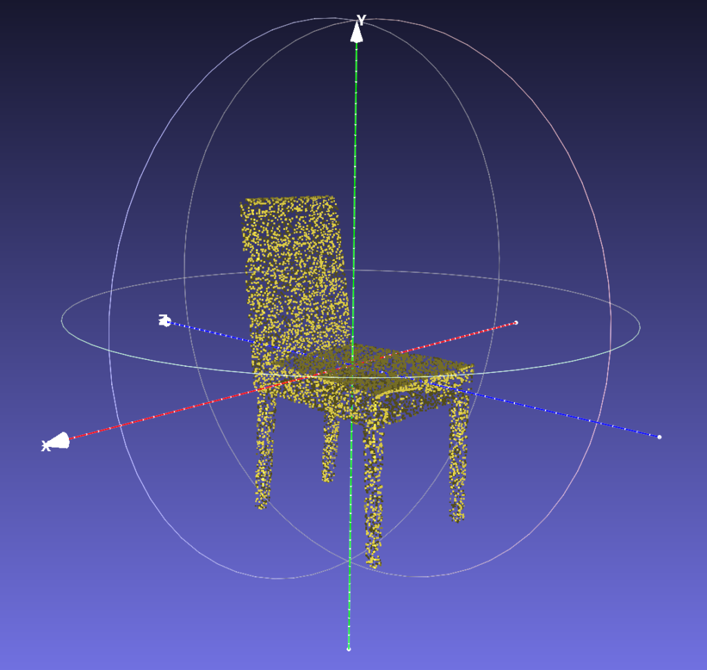
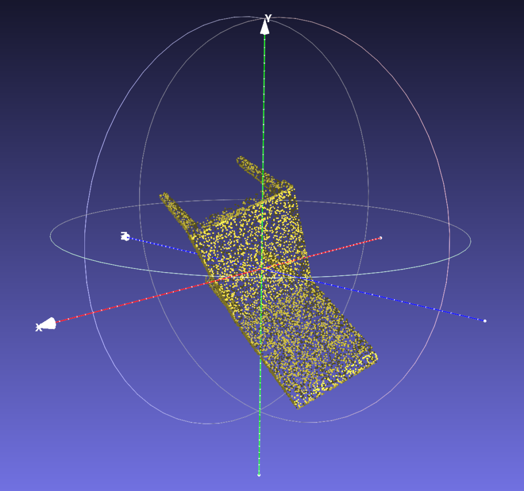
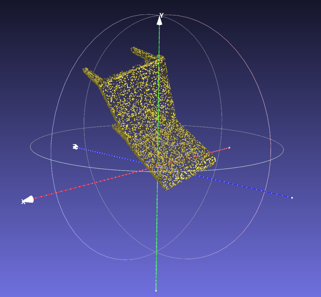
Following the implementation described above, we trained a classification model on 5 selected classes (bed, chair, sofa, table, toilet) in the ModelNet40 dataset. We obtained a Vector Neurons classification model with the same PointNet backbone (input and feature transformation included) pre-trained on the complete ModelNet40 dataset. We tested the classification accuracy on both models with point cloud data of the 5 selected classes randomly transformed by rotation-only or rotation and translation. The results are shown in the table below.
Original Point Cloud of ChairRotation-onlyRotation and Translation
SO(3) Test Instance Accuracy
SE(3) Test Instance Accuracy
Vector Neurons
89.6%
6.1%
Frame Averaging
80.7%
80.3%
The Vector Neurons model was trained for a more difficult classification task, but it was also more fined tuned with a much longer training time and larger data size. The Frame Averaging model in our experiment, however, was trained with relatively larger learning steps and shorter training time. Although it is not fair to make a direct comparison between the two models, we can still see a conclusive result. As expected, the Vector Neurons model has good SO(3) invariance, but tends to fail when the point cloud is translated. The Frame Averaging model, on the other hand, performs similarly well on both SO(3) and SE(3) invariance tests.
If the Frame Averaging model was trained with the same setting as the Vector Neurons model, we believe that it will have both the accuracy of SO(3) and SE(3) tests comparable with Vector Neurons’ SO(3) accuracy, because of its maximal expressive power. Due to the limited resource, we cannot prove our hypothesis by experience, but we will provide more theoretical analysis in the next section.
Discussion: Expressive Power of Frame Averaging
Besides the good performance in maintaining SE(3) invariance in classification tasks, we want to further discuss the advantage of frame averaging, namely its ability to preserve the expressive power of any backbone architecture.
The Expressive Power of Frame Averaging
Let \(\phi: V \rightarrow \mathbb{R}\) and \(\Phi: V \rightarrow W\) be some arbitrary functions, e.g. neural networks where \(V, W\) are normed linear spaces. Let \({G}\) be a group with representations \(\rho_1: G \rightarrow GL(V)\) and \(\rho_2: G \rightarrow GL(W)\) that preserve the group structure.
Definition
A frame is bounded over a domain \(K \subset V\) if there exists a constant \(c > 0\) so that \(||\rho_2(g)|| \leq c\) for all \(g \in F(X)\) and all \(X \in K\) where \(||\cdot||\) is the operator norm over \(W\).
A domain \(K \subset V\) is frame finite if for every \(X \in K\), \(F(X)\) is a finite set.
A major advantage of Frame Averaging is its preservation of the expressive power of the base models. For any class of neural networks, we can see them as a collection of functions \(H \subset C(V,W)\), where \(C(V,W)\) denotes all the continuous functions from \(V\) to \(W\). We denote \(\langle H \rangle = \{ \langle \phi \rangle | \phi \in H\}\) as the transformed \(H\) after applying the frame averaging. Intuitively, the expressive power tells us the approximation power of \(\langle H \rangle\) in comparison to \(H\) itself. The following theorem demonstrates the maximal expressive power of Frame averaging.
Theorem
If \(F\) is a bounded \(G\)-equivariant frame over a frame-finite domain \(K\), then for any equivariant function \(\psi \in C(V,W)\), the following inequality holds
where \(K_F = \{ \rho_1(g)^{-1}X | X \in K, g \in F(X)\}\) is the set of points sampled by the FA operator and $c$ is the constant from the definition above.
With the theorem above, we can therefore prove the universality of the FA operator. Let \(H\) be any collection of functions that are universal set-equivariant, i.e., for arbitrary continuous set function \(\psi\) we have \(\inf_{\phi \in H} ||\psi – \phi||_{\Omega,W} = 0\) for arbitrary compact sets \(\Omega \subset V\). For bounded domain \(K \subset V\), \(K_F\) defined above is also bounded and contained in some compact set \(\Omega\). Therefore, we can conclude with the following corollary.
Corollary
Frame Averaging results in a universal SE(3) equivariant model over bounded frame-finite sets, \(K \subset V\).
In the first week of project SE(3) Invariant and Equivariant Neural Network for Geometry Processing, we studied the research approach frame averaging that tackles the challenge of representing intrinsic shape properties with neural networks. Here we introduce the paper Frame Averaging for Invariant and Equivariant Network Design[1] which grounded the theoretical analysis of generalizing frame averaging with different data types and symmetry groups.
Motivation
Deep neural networks are useful for approximating unknown functions with combinations of linear and non-linear units. Its application, especially in geometry processing, involves learning functions invariant or equivariant to certain symmetries of the input data. Formally, for a function \(f\) to be
invariant to transformation \(A\), we have \(f(Ax)=f(x)\);
equivariant to transformation \(A\), we have \(f(Ax)=Af(x)\).
This paper introduced Frame Averaging (FA), a systematic framework for incorporating invariance or equivariance into existing architecture. It was derived from the observation in group theory that
Arbitrary functions \(\phi:V\rightarrow\mathbb{R}, \Phi:V\rightarrow W\), where \(V, W\) are some vector spaces, can be made invariant or equivariant by symmetrization, that is averaging over the group.
Instead of averaging over the entire group \(G\) with potentially large cardinality, where exact averaging is intractable, the paper proposed an alternative of averaging over a carefully selected subset \(\mathcal{F}(X)\subset G\) such that the cardinality \(|\mathcal{F}(X)|\) is small. Computing the average over \(\mathcal{F}(X)\) can efficiently retain both the expressive power and the exact invariance/equivariance.
Frame Averaging
Let \(\phi\) and \(\Phi\) be arbitrary functions, e.g. neural networks.
Let \({G}\) be a group with representation \({p_i}\)’s that preserves the group structure by satisfying \({p_i}(gh)= {p_i}(g){p_i}(h)\) for all \({g}, {h}\) in \({G}\).
We want to make
\(\phi\) into an invariant function, i.e. \(\phi(p_1(g){X})= \phi({X})\); and
\(\Phi\) into an equivariant function, i.e. \(\Phi(p_1(g){X})= {p_2(g)}\Phi({X})\).
Instead of averaging over the entire group each time, we will do that by averaging over group elements. Specifically, we will take the average on a subset of the group elements – called a frame.
A frame is defined as a set valued function \(\mathcal{F}:V\rightarrow\ {2^G \setminus\emptyset}\).
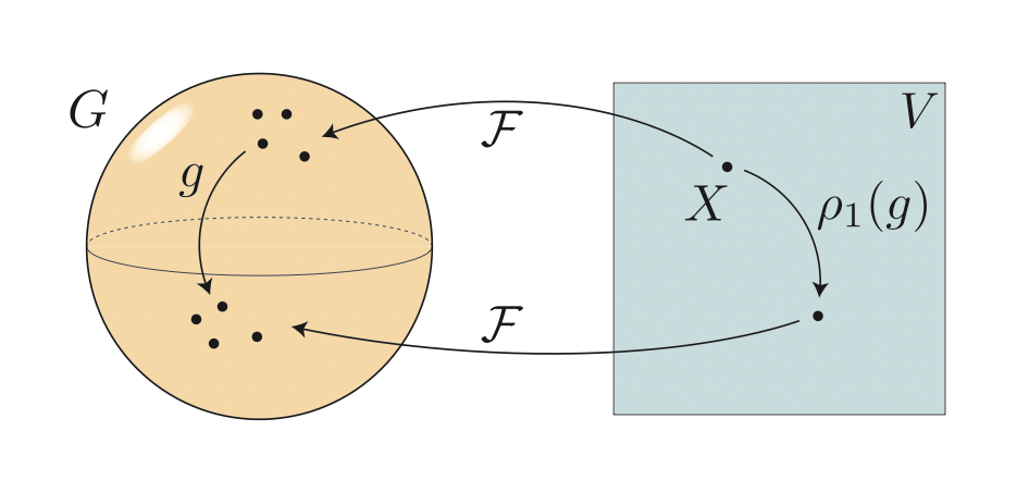
A frame is \(G\)-equivariant if \(F(\rho_1(g)X) = gF(X)\) for every \(X \in V\) and \(g \in G\) where\(gF(X)= \{gh|h \in F(X)\}\) and the equality means that the two sets are equal.
Why are the equivariant frames useful?
Figure 1: Frame equivariance (sphere shape represents the group \(G\); square represents \(V\)).
If we have a case where the equivariant frame is easy to compute, and its cardinality is not too large, then averaging over the frame, provides the required function symmetrization. (for invariance and equivariance).
Frame Averaging
Let \(\mathcal{F}\) be a \({G}\) equivariant frame, and \(\phi:V\rightarrow\mathbb{R}, \Phi:V\rightarrow W\) be some functions.
Then, \(\langle \phi \rangle _F\) is \(G\) invariant, while \(\langle \Phi \rangle _F\) is \(G\) equivariant.
Incorporating G as a second symmetry
Here, we have \(\phi, \Phi\) that is already invariant/equivariant w.r.t. some symmetry group \(H\). We want to make it invariant/equivariant to \(H × G\).
Frame Average second symmetry
Let \(\mathcal{F}\) be a \({G}\) equivariant frame, and \(\phi:V\rightarrow\mathbb{R}, \Phi:V\rightarrow W\) be some functions.
Then, \(\langle \phi \rangle _F\) is \(G\) invariant, while \(\langle \Phi \rangle _F\) is \(G\) equivariant.
Assume \(F\) is \(H\)-invariant and \(G\)-equivariant. Then,
If \(\phi:V\rightarrow\mathbb{R}\) is \(H\) invariant, and \(ρ_1,τ_1\) commute, then \(\langle \phi \rangle _F\) is \(G×H\) invariant.
If \(\Phi:V\rightarrow W\) is \(H\) equivariant and \(ρ_i, τ_i, i = {1,2}\), commute then \(\langle \Phi \rangle _F\) is \(G×H\) equivariant.
Efficient calculation of invariant frame averaging
We can come up with a more efficient form of FA in the invariant case.
The stabilizer of an element \(X∈V\) is a subgroup of \(G\) defined by \(G_X =\{g∈G∣ρ_1(g)X=X\}.\) \(G_X\) naturally induces an equivalence relation ∼ on \(F(X)\), with \(g ∼ h ⇐⇒ hg^{−1} ∈ G_X.\) The equivalence classes (orbits) are \([g] = {h ∈ F(X)∣g ∼ h} = G_Xg ⊂ F(X), for g∈F(X)\), and the quotient set is denoted \(F(X)/G_X.\)
Equivariant frame \(F(X)\) is a disjoint union of equal size orbits, \([g] ∈ F(X)/G_X\).
Approximation of invariant frame averaging
When \(F(X)/G_X\) is hard to enumerate, we can draw a random element from \(F(X)/G_X\) with uniform probability.
Let \(F(X)\) be an equivariant frame, and \(g ∈ F(X)\) be a uniform random sample. Then \([g] ∈ F(X)/G_X\) is also uniform.
Hence, we get an efficient approximation strategy that is averaging over uniform samples.
Model Instances
An instance of the FA framework contains:
The symmetry group \(G\), representations \(\rho_1,\rho_2\) , and the underlying frame \(\mathcal{F}\).
The backbone architecture for \(\phi\) (invariant) or \(\Phi\) (equivariant).
Example: Normal Estimation with Point Cloud
Here we use normal estimation with point cloud data as an example. The goal is to incorporate \(E(d)\) equivariance to the existing backbone architecture (e.g. PointNet and DGCNN).
Mathematical Formulation
The paper proposed the frame \(\mathcal{F}(X)\) based on Principal Component Analysis (PCA). Formally, we present the centroid of \(X\) by
$$t=\frac{1}{n}X^T\mathbf{1}\in\mathbb{R}^d $$
$$t=\frac{1}{n}X^T\mathbf{1}\in\mathbb{R}^d $$
and covariance matrix computed after centering the data is
where \(\mathbf{v}_1, …, v_d\) are the eigenvectors of \(C\). From that, we can form the representation for the frames as transformation matrices.
$$\rho(g)=\begin{pmatrix}R & t \\\mathbf{0}^T & 1\end{pmatrix}, R=\begin{bmatrix}\alpha_1v_1 &…&\alpha_dv_d\end{bmatrix} $$
Implementation
We show part of the implementation of normal estimation for point cloud in PyTorch. For more details, please refer to the open-source code provided by the authors of [1].
We first perform PCA with the input point cloud.
# Compute the centroid
center = pnts.mean(1,True)
# Center the points
pnts_centered = pnts - center
# Compute covariance matrix
R = torch.bmm(pnts_centered.transpose(1,2),pnts_centered)
# Eigen-decomposition
lambdas,V_ = torch.symeig(R.detach().cpu(),True)
# Reshape the eigenvectors
F =  V_.to(R).unsqueeze(1).repeat(1,pnts.shape[1],1,1)
Finally, we perform the preprocessing to the point cloud data by centering and computing the frame average.
pnts_centered = point_cloud - center

# Apply inverse of the frame operation
framed_input = torch.einsum('bopij,bpj->bopi',F_ops.transpose(3,4),pnts_centered)

# feed forward to the backbone neural network
# e.g. point net
outs = self.nn_forward(framed_input)

# Apply frame operation
outs = torch.einsum('bopij,bopj->bopi',F_ops,outs)

# Take the average
outs = outs.mean(1)
For a more detailed example application of frame averaging, please see the next blog post by our group: Frame Averaging for Invariant Point Cloud Classification.
[1] Omri Puny, Matan Atzmon, Heli Ben-Hamu, Ishan Misra, Aditya Grover, Edward J. Smith, and Yaron Lipman. Frame averaging for invariant and equivariant network design. In ICLR, 2022.
In industry CAD (Computer-Aided Design) representation for 3D models is very used, and it is estimated that about 80% of overall analysis time is devoted to mesh generation in the automotive, aerospace and shipbuilding industries. But, the geometric approximation can lead to accuracy problems and the construction of the finite element geometry is costly, time-consuming and creates inaccuracies.
Isogeometric Analysis (IGA) is a technique that integrates FEA (Finite Element Analysis) into CAD (Computer-Aided Design) models, enabling the model to be designed and tested using the same domain representation. IGA is based on NURBS (Non-Uniformal RAtional B-Splines) a standard technology employed in CAD systems. One of the benefits of using IGA is that there is no approximation error, as the model representation is exact, unlike conventional FEA approaches, which need to discretize the model to perform the simulations.
For our week 4 project we followed the pipeline described in Yuxuan Yu’s paper [1], to convert conventional triangle meshes into a spline based geometry, which is ready for IGA, and we ran some simulations to test it.
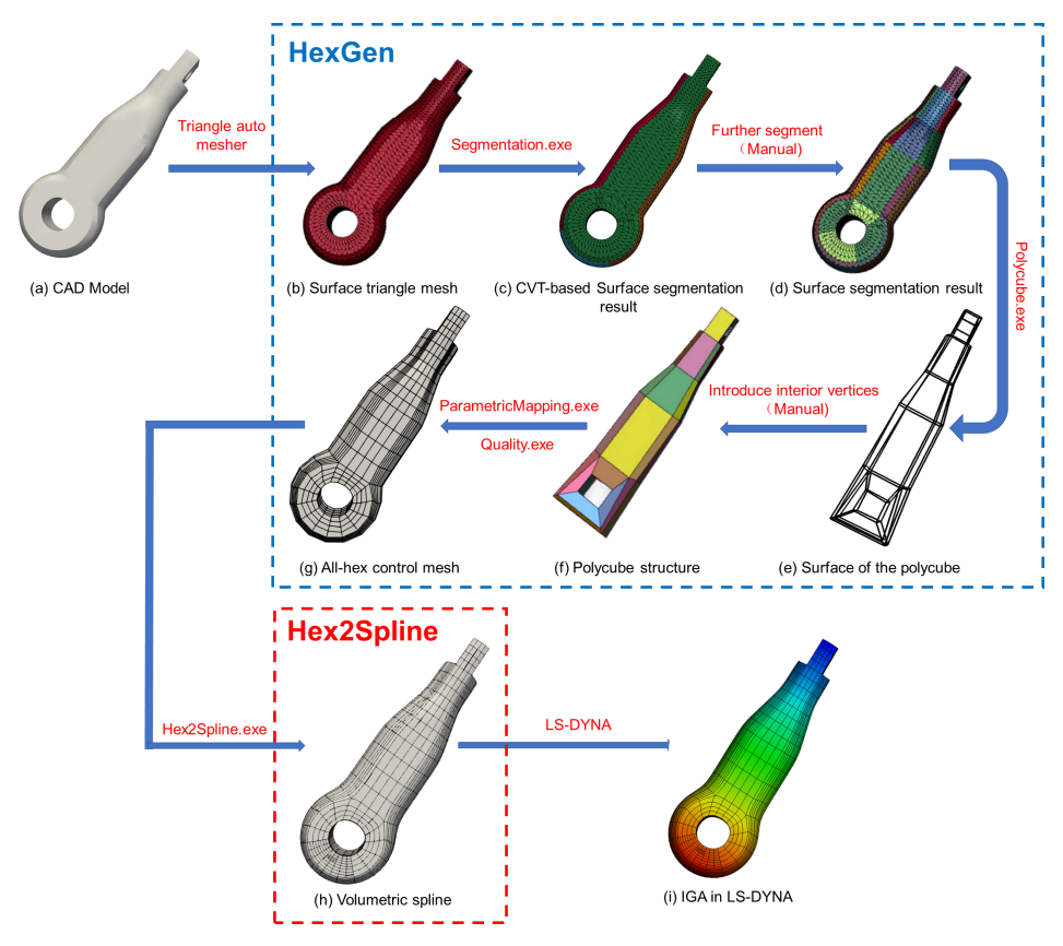
The general pipeline consists of two parts: the HexGen, which transforms a CAD Model into a All-Hex Mesh, and the Hex2Spline, which transforms the All-Hex Mesh into a Volumetric Spline, ready for IGA. The code can be found here GitHub – SGI-2022/HexDom-IGApipeline.
HexGen and Hex2Spline pipeline
Following the pipeline
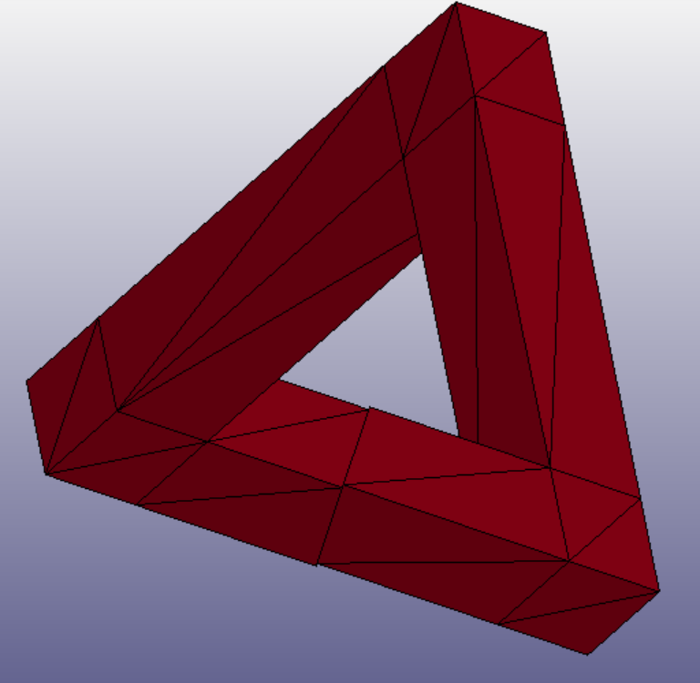
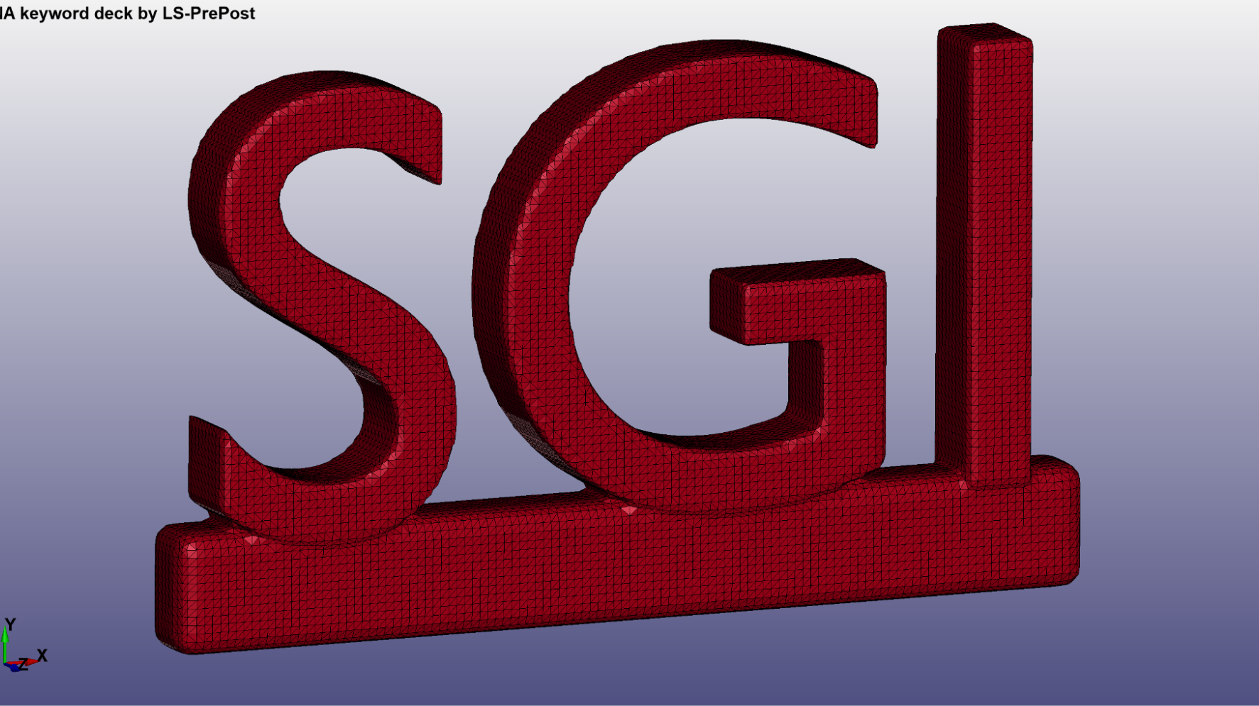
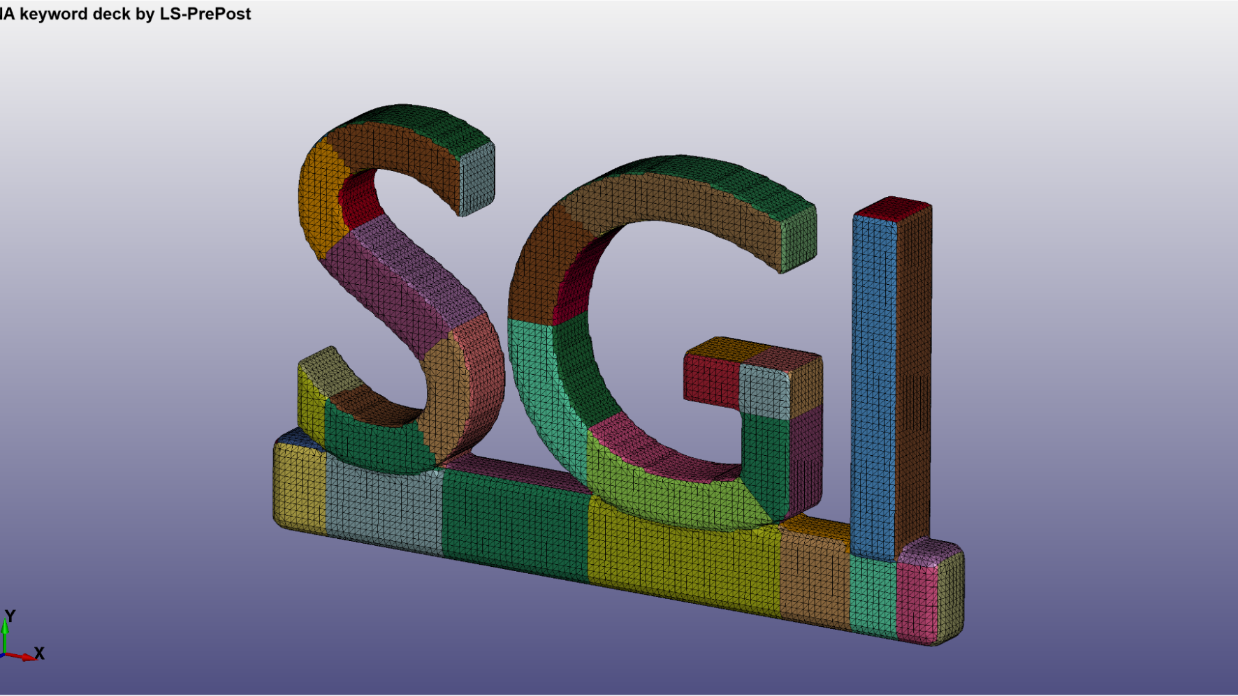
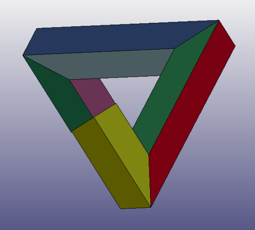
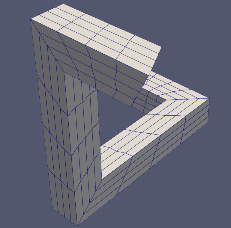
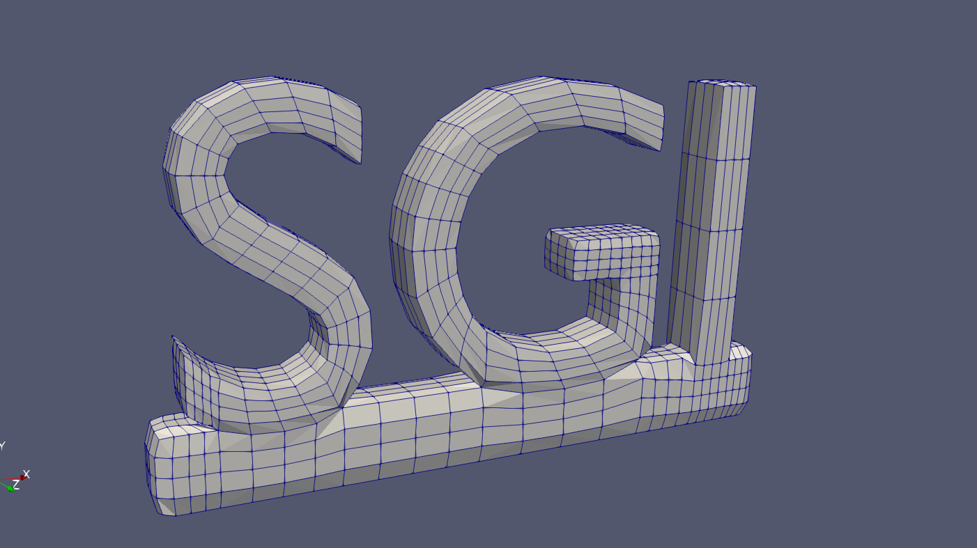
For testing the pipeline, we reproduced the steps with our own models. LS-prepost was used to visualize and edit the 3D models. We started with two surface triangle mesh:
Penrose triangle meshSGI triangle mesh
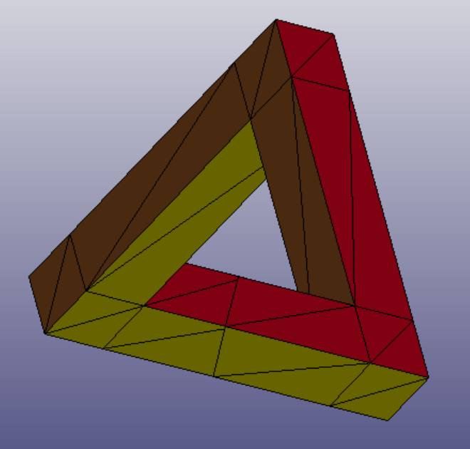
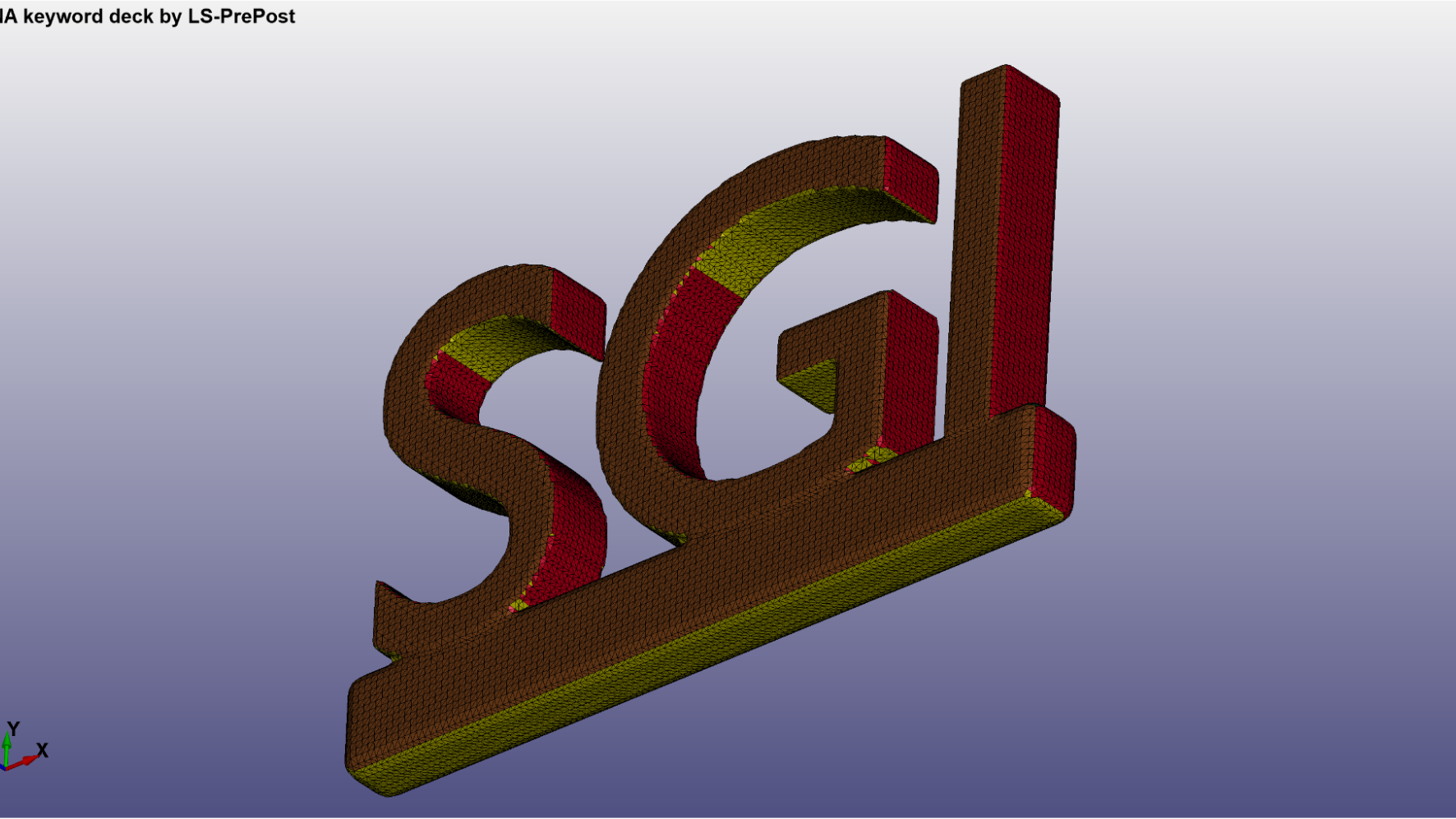
The first step of the pipeline is using a surface segmentation algorithm based on CVT (Centroidal Voronoi Tessellation), using the Segmentation.exe script. It was used to segment the triangle mesh into 6 regions, one for each of the three principal normal vectors and their opposite normals (±𝑋, ±𝑌, ±𝑍).
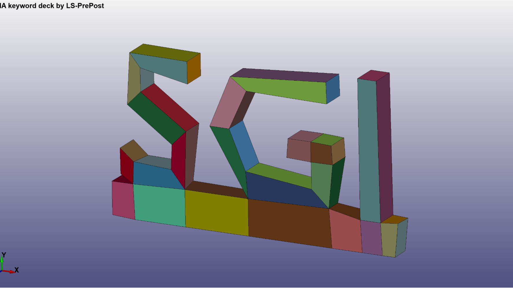
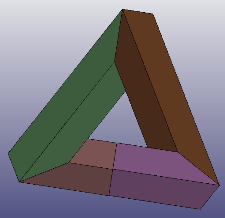
The initial segmentation only generates 6 clusters, and for more complex shapes we need a better segmentation to later build a polycube structure. Therefore, a more detailed segmentation is done, trying to better divide the mesh into regions that can be represented by polycubes. This step is done manually.
Penrose segmentationSGI segmentation
Now it is clearly visible which are the faces for the polycube structure. We can now apply a linearization operation on the segmentation, using the Polycube.exe script.
After that, we join the faces to create the cubes and finally have our polycube structure. This step is also done manually. The image in the right represents the cubes decreased in volume, for better visualization.
Penrose polycube structureSGI polycube structure
Then we want to build a parametric mapping between polycube and CAD model, which takes as input the triangle mesh and the polycube structure, to create an all-hex mesh. For that, we use the ParametricMapping.exe script.
Penrose all-hex meshSGI all-hex mesh
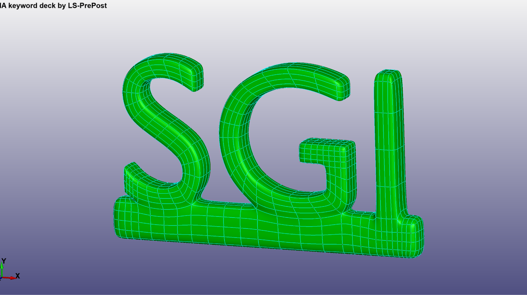
And in the last step, we use the Hex2Spline.exe script to generate the splines.
Penrose splineSGI spline
For testing the Splines, we performed a Modal Analysis (simple eigenvalue problem) in each of them, using the LS-DYNA simulator. An example for a specific displacement can be seen below:
Penrose modal analysis
SGI modal analysis
Improvements for the pipeline
The pipeline used still have two manual steps: the segmentation of the mesh, and building the polycube structure given the linear surface segmentation. During the week, we thought and discussed some possible approaches to automate the second step. Given the external faces of the polycube structure, we need to recover the volumetric information. We came up with a simple approach using graphs, representing the polycubes as vertices, the internal faces as edges, and using the external faces to build the connectivity between the polycubes.
Although, this approach doesn’t solve all the cases, for example, when a polycube consists mostly of internal faces, and are not uniquely determined. And even if we automated this step, the manual segmentation process still is a huge bottleneck in the pipeline. One solution to the problem would be generating the polycube structure directly from the mesh, without the need of a segmentation, but it’s a hard problem to automatically build a structure that doesn’t have a big amount of polycubes and still represents well the geometry and topology of the mesh.
By Mariem Khlifi, Abraham Kassahun Negash, Hongcheng Song, and Qi Zhang
Introduction
For two weeks, we were involved in a project that looked at an interesting way of extracting lines from a line drawing raster image, mentored by Mikhail Bessmeltsev and Edward Chien and assisted by Zhehao Li.
Despite its advent in the 90s, automatic line extraction from drawings is still a topic of research today. Due to the unreliability of current tools, artists and engineers often trace lines by hand rather than deal with the results of automatic vectorization tools.
Most past algorithms treat junctions incorrectly which results in incorrect topology, which can lead to problems in applying different tools to the vectorized drawing. Bessmeltsev and Solomon [1] looked at junction detection as well as vectorizing line drawings using frame fields. Frame fields assign two directions to each point, one direction tangent to the curve and the other roughly aligned to neighboring frame field directions. This second direction is important at junctions as it aligns with the tangent of another incoming curve.
We tried to build on this work by additionally looking at minimal currents. Currents are functionals over the space of differential forms on a smooth manifold. They can be thought of as integrations of differential forms over submanifolds. Wang and Chern [2] represented surfaces bounded by curves as differential forms, leading to a formulation of the Plateau problem whose optimization is convex. This representation is common in geometric measure theory, which studies the geometric properties of sets in some space using measure theory. We used this procedure to find curves in our 2D space with a given metric that minimized the distance between two points. The formulation for a flat 2D space is similar to that of the paper, but some modifications had to be made in order to introduce a narrow band metric or frame fields (i.e. to obtain a curve that follows the dark lines while trying to minimize distance).
Theory
Vectorization using Frame Fields
Frame fields help guide the vectorized line in the direction of the drawn line. First, a gradient of the drawing is defined based on the intensity of the pixel. One of the frame field directions is optimized to be as close as possible to the direction perpendicular to this gradient while being smooth. The second direction is determined by a compromise between a few rules we want to enforce. First, this direction wants to be perpendicular to the tangent direction. Second, it wants to be smooth. For example, at a junction where we have a non-perpendicular intersection, the second direction starts to deviate from the perpendicular before the intersection so that it aligns with the incoming curve at the intersection.
Bessmeltsev and Solomon used these frame fields to trace curves along the tangent direction and bundle the extracted curves into strokes. The curves were obtained using Euler’s method by tracing along the tangent direction from each point up to a certain step size.
We on the other hand looked at defining a metric at each frame which defines the cost of moving in each direction. We then move through the frame field and try to minimize the distance between our start and end points. In this manner the whole drawing can be vectorized given we have the junction points and the frame field.
What are differential forms?
The main focus of our project was to understand and implement the algorithm proposed by Wang and Chern for the determination of minimal surfaces bounded by a given curve. We reduce the dimension to suit our application and add a metric so that the space is no longer Euclidean.
The core idea of their method is to represent surfaces using differential forms. Differential forms can be thought of as infinitesimal oriented lengths, areas or volumes defined at each point in the space. They can also be thought of as functions that take in vectors, or higher dimensional analog of vectors, and output scalars. In this interpretation, they can be thought of as measuring the vector or vector analog.
A k-form can be defined on an n-dimensional manifold, where k = 0,1,2,…,n. A 0-form is just a function defined over the space that outputs a scalar. 1-forms also known as covectors, which from linear algebra can be recalled to live inside the dual space of a vector space, map vectors to scalars. Generally, a k-form takes in a k-vector and outputs a scalar. These k-vectors are higher dimensional extensions of vectors that can be described by a set of k vectors. They have a magnitude defined by the volume spanned by the vectors. Additionally, they have an orientation, thus in general they can be thought of as signed k-volumes.
k-forms can be visualized as the k-vectors they measure, and the measurement operation can be thought of as taking the projection of the k-vector onto the k-form. But it is important to realize these are two different concepts even if they behave similarly. Their difference is clearly seen in curved spaces. Musical isomorphisms relate a k-form to a k-vector by taking advantage of this similarity, where a \(\sharp\) takes a k-vector to a k-form while a \(\flat\) takes a k-form to a k-vector.
We can define the wedge product denoted by \(\wedge\) to describe the spanning operation described earlier. In particular, a k-vector spanned by vectors x1, x2, x3,…,xk can be expressed as \(x_1 \wedge x_2 \wedge . . . \wedge x_k\).
An operation called the Hodge star denoted by \(\star\) can also be defined on forms. On an n-dimensional space, the Hodge star maps a k-form to an n-k-form. In this way, it gives a complementary form.
Reformulation of the plateau problem
Plateau’s problem can be stated as follows. Given given a closed curve \(\Gamma\) inside a 3-dimensional compact space M, find the oriented surface \(\Sigma\) in M such that its area is minimal.
Wang and Chern represent the surface \(\Sigma\) and curve \(\Gamma\) using Dirac-delta forms \(\delta_\Sigma\) and \(\delta_\Gamma\). These are a one- and a two-form, respectively, having infinite magnitudes at the surface and 0 everywhere else. They can be understood as the forms used to measure line and surface integrals of vector fields on the curve and surface. Then they take the mass norm of this Dirac-delta form which is equivalent to the area of the surface. Thus minimizing this mass norm is the same problem as minimizing the area of the surface. The area can be expressed as:
Now, it happens that solving the Poisson equation features a bit in our solution algorithm, and to speed this process up, using a Fast Fourier Transform is advantageous. To use FFT, however, we need to use a periodic boundary condition. This introduces solutions that we might not necessarily want which belong to a different homology class to our desired solution. To alleviate this solution, Wang and Chern impose an additional constraint that ties the cohomology class of the optimum 1-form to the initial 1-form.
Finally, the space of 1-forms can be decomposed into coexact, harmonic and exact parts by the Helmholtz-Hodge decomposition, which simplifies all the constraints into a single constraint. After some rearranging, we arrive at the following final form.
Given an initial guess \(\eta_0 \in \Omega^1 (M)\) satisfying \(d\eta_0 = \delta_\Gamma\) and \(\int_{M} \vartheta_i \wedge \star \eta_0 = \Lambda_i\), solve
Even though we are working on a 2-dimensional space, the final form of the Plateau problem is identical in our case as well. Unlike Wang and Chern, who were working in 3D, we didn’t need to worry as much about the initial conditions as we can initialize plausible one-forms by defining an arbitrary curve between two points and taking the one form to be perpendicular to the curve at each vertex and oriented consistently.
The Algorithm
Algorithm 1 (Main Algorithm)
Our goal is to solve the Plateau problem \(\min_{\eta \in \eta_0 + im(d^0)} ||\eta||_{mass}\). This boils down to adding a component to an initial guess. So, an initial guess will already give us a good estimation of how to solve the problem by adjusting the solution values through optimization principles. In this sense, our final solution is the initial guess plus a certain component dφ:
The algorithm then tries to solve \(\min_{\varphi \in \mathbb{R}^V, X \in \mathbb{R}^{V \times 3}} ||X||_{L^1}\), subject to \(D\varphi – X = -X_0\) where \(X\) is the discrete form of the one-form \(\eta\) and \(V\) is the number of vertices in the space after discretizing..
Lagrange multipliers are introduced to reinforce the constraints and act as multipliers that relate the gradient of the \(X\) variable and the constraints since in general, their gradients point towards the same direction. Generally, the optimization is done in one go. However, since we are solving a minimization problem with two unknown components \(X\) and \(\varphi\), we resort to Alternating Direction Method of Multipliers (ADMM), which adopts a divide and conquer approach that decouples the two variables and solves each one of them in an alternating fashion until X converges [3]:
For the initialization, we have created our own 2D path initializer which takes two points and creates an L-shaped path. The corresponding 1-form consists of the normals perpendicular to the path and \(X_0\) is obtained through integration over the finite region surrounding each vertex. More complex paths can be created by adding the 1-forms related to multiple L-shaped segments.
Throughout the paper, the convention used for integration to evaluate \(X\) from 𝜂 and differentiation to define the differentiation matrices for the Poisson solver was the midpoint approach. We have noticed however, that a forward or backward differentiation produced more accurate results in our case.
Algorithm 2 (Poisson Solver)
To solve for \(\varphi\) we reduce the following equation we have from the ADMM optimization.
where \(\Delta=D^TD\), and \(D\) is the finite difference differential operator using central difference. Because the Fast Fourier Transform (FFT) is computation friendly to the computation of derivatives of our PDE or ODE by its clean and clear formula, we use FFT to solve the Poisson equation. Our FFT Poisson solver projects the right hand side signal from the time domain onto a different finite frequency basis in the frequency domain, and the solution is simply a scalar product in the frequency domain. The final solution in the time domain is generated by the inverse FFT.
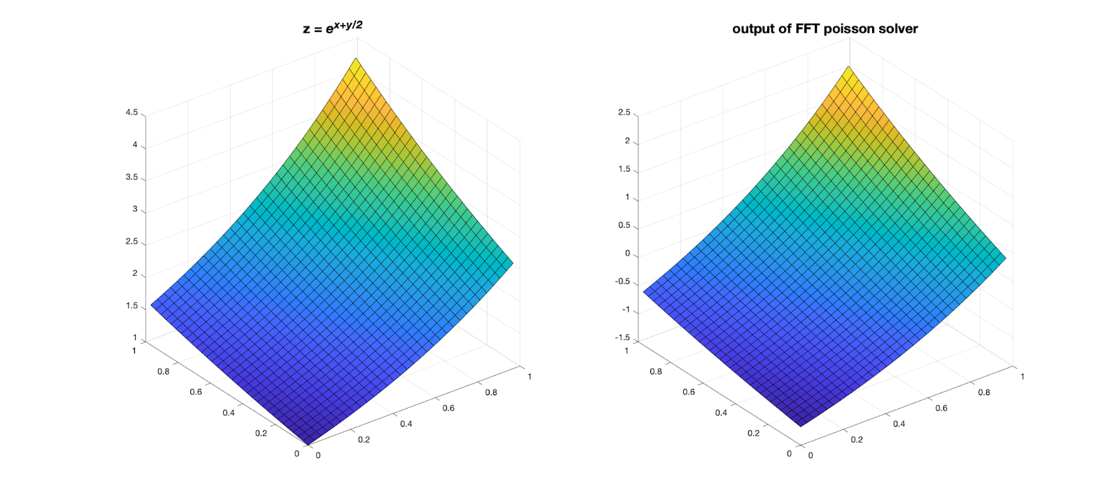
To test the validity of the FFT Poisson solver, we use \(z = exp(x+\frac{y}{2})\) as the original function and compute its Laplacian as the right hand side signal. The final solution is identical up to a constant value (-2.1776), which is easy to find in the (0, 0) point.
Fig 2: Validation of the Poisson solver
Algorithm 4 (Shrinkage)
Now for the minimization of X, we remember the formula we obtained earlier.
Where \(z = \tau \hat{\lambda}_v + (D\varphi)_v + (X_0)_v\)
This minimizes the euclidean distance, which is only helpful for drawing lines. To adjust the formulation for our case where the defined metric and the Euclidean metric are different, we first update the minimization problem to include the newly defined metric and then solve it to obtain the new formulation of the Shrinkage map.
Results
After we tinkered with the algorithm, we felt that it was time that we sent it to kindergarten to learn a few tricks.
Drawing a line
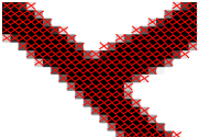
For this example, we define two points as our boundary and take a non-optimal path (sequence of segments) between them as our initial guess. Once this path is determined, we find its equivalent 1-form which extracts the normals at every vertex of our grid with respect to the path. The metric used in this example is the Euclidean metric, i.e., it’s constant everywhere, so the optimal path will be a line connecting the boundary points.
Fig 3: Initial one-form(top left) pseudo-inverse of the minimizing one-form (top-right) level-set obtained from the pseudo-inverse(bottom-left) minimizing one-form (bottom-right)
Note that to obtain the curve, we take the pseudo-inverse of the final one-form \(X\). This gives a 0-form which can be visualized as a surface. This surface will have a big jump over the curve we are looking for.
Tracing a circle
Instead of relying on a Euclidean metric, we can define our own metric to obtain the connecting line within a certain narrow band instead of getting the straight line that connects two points. A narrow band allows us to define pixels that should be prioritized over others. It defines in some way a penalty if the algorithm passes through a section that is not part of the narrowband by making it more expensive to go through these pixels in comparison to choosing the pixels from the narrowband.
We need to update our shrinkage problem. If \(c\) is the cost associated with each pixel, then the equation for \(X\) becomes:
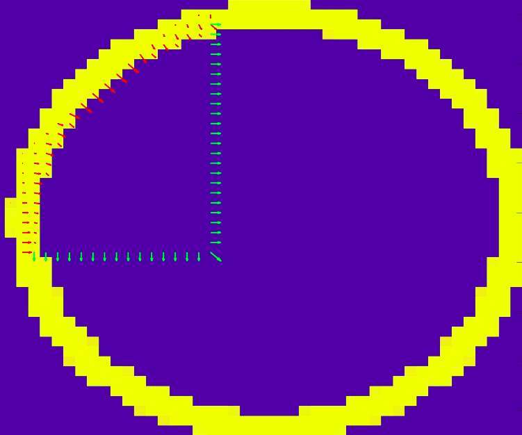
Fig 4: Superimposition of the initial one-form(green normals), final one-form(red normals) and narrow band(yellow)
Same boundary, multiple paths
The algorithm provides a unique solution to the problem, which means that with different initial solutions for the same boundary, we obtain the same solution. We proved this by defining two curves having the same boundary (in 2D, our boundary is two points).
Fig 5: The initializing one-form as a Superposition of two one-forms corresponding to two curves between the boundaries.
Fig 6: minimizing one-form(top left) pseudo-inverse of the minimizing one-form (top-right) level-set obtained from the pseudo-inverse(bottom-left)
Crossing paths
We have defined two intersecting paths from points from the circle. The obtained paths connected points that were not connected in the initialization. This shows the importance of running the optimization on points separately to obtain results on-par with the model’s complexity.
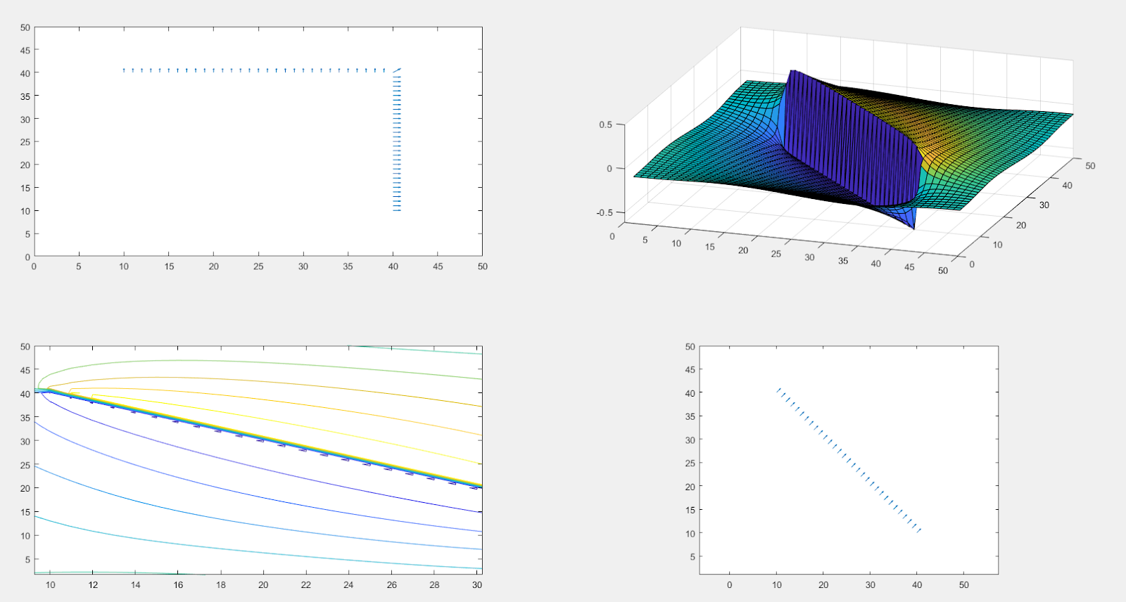
Fig 7: minimizing one-form(top left) pseudo-inverse of the minimizing one-form (top-right) level-set obtained from the pseudo-inverse(bottom-left) initial one-form superimposed on the narrow band (bottom-right)
Cross-Shaped Narrow Band
We define crossing paths similar to the point above but we change the shape of the narrow band to a cross. The result yields connections between the closest points in the narrow band, hence the hyperbolic appearance.
Fig 8: Initial one-form(top left) initial one-form superimposed on the narrow band (top-right) level-set obtained from the pseudo-inverse(bottom-left) minimizing one-form (bottom-right)
Conclusion
We have successfully used an algorithm proposed by Wang and Chern [2] for curves instead of surfaces to find minimal connections between 2D boundaries while also incorporating metric information from narrow bands to obtain various shapes of these connections. We have enjoyed working on this project which combined many topics that were new to us and we hope that you have similarly enjoyed going through the blog post!
In this blog, we explain how we can train SIREN architecture on a 3D point cloud (Dragon object), from The Stanford 3D Scanning Repository. This work had been done during the project “Implicit Neural Representation (INR) based on the Geometric Information of Shapes” SGI 2022, with Alisia Lupidi and Krishnendu Kar, under the guidance of Dr. Dena Bazazian and Shaimaa Monem Abdelhafez.
Introduction
The SIREN architecture is a neural network with a periodic activation function that has been proposed to reconstruct 3D objects, and considered as a signed distance function (SDF). We train this network using a colab notebook to reconstruct a Dragon object, which we take from The Stanford 3D Scanning Repository. We provide the instructions to produce our experiments.
Note: you have to use a GPU for this experiment. If you use Google Colab, you just set your runtime to GPU.
Instructions to run our experiments
First, you have to clone the SIREN repository in your notebook using the code below,
git clone https://github.com/vsitzmann/siren
After cloning the repository, install the required libraries by:
Then, you can download the Dragon object from The Stanford 3D Scanning Repository (you can also try another 3D object). The 3D object has to be converted to xyz format, for which you can use MeshLab.
The next step is to train the neural network (SIREN) to reconstruct the 3D object. You can achieve this task by running the following script:
The reconstructed point cloud file will be saved in the folder “experiment_1_rec”. Here is also visualization for the reconstructed Dragon (in gray) wrt to the original one (in brown) using MeshLab. Where you can notice the reconstructed version has a larger scale.
The reconstructed Dragon (in gray) wrt to the original one (in brown) using MeshLab.