Munshi Sanowar Raihan

Fellows: Munshi Sanowar Raihan, Daniel Perazzo, Francheska Kovacevic, Gabriele Dominici

Volunteer: Elshadai Tegegn

Mentors: Silvia Sellán, Dena Bazazian

I. Introduction

In computer graphics, fracture simulation of everyday objects is a well-studied problem. Physics-based pre-fracture algorithms like Breaking Good [1] can be used to simulate how objects break down under different dynamic conditions. The inverse of this problem is geometric fracture assembly, where the task is to compose the components of a fractured object back into its original shape.

More concretely, we can formulate the fracture assembly task as a pose prediction problem. Given \(N\) mesh fractured pieces of an object, the goal is to predict a \(SE(3)\) pose for each fractured part. We can denote the predicted pose of the \(i_{th}\) fractured piece as \(p_i = \{(q_i, t_i) | q_i \in R^4, t_i \in R^3\}\), where \(q_i\) is a unit quaternion describing the rotation and \(t_i\) is the translation vector. We can apply the predicted pose to the vertices \(V_i\) of each fractured piece and get \(p_i(V_i) = q_i V_i q_i^{-1} + t_i\). The union of all of the pose-transformed pieces is our final assembly result, \(S = \bigcup p_i(V_i)\).

The goal of this project is to come up with an evaluation metric to compare different assembly algorithms and to host an open source challenge for the assembly task.

II. Rotation metric:

We will use unit quaternions \(q\) to represent rotations. Let’s assume for one of the pieces of the fracture, \(q_r\) is the true rotation and \(q_p\) is the predicted rotation. We might define a metric between two rotations as the Euclidean distance between two quaternions:

\(d(q_r, q_p) = ||q_r-q_p||^2\)

But a noteworthy property of quaternions is that two quaternions \(q\) and \(-q\) represent the same rotation. This can be verified as follows:

The rotation \(R\) related to quaternion \(q\) sends a vector \(v\) to the vector:

\(R(v) = qvq^{-1}\)

The rotation \(R’\) related to quaternion \(-q\) sends the vector \(v\) to the vector:

\begin{array} {lcl} R'(v) & = & (-q)v(-q)^{-1} \\ & = & (-1)^2 qvq^{-1} \\ & = & qvq^{-1} \end{array}

Which is the same as the rotation \(R\).

Directly using the Euclidean distance for quaternions would be ambiguous because the distance between the same rotations \(q\) and \(-q\) would be non-zero.

To alleviate this, we have to choose a sign convention for the quaternions. We choose the quaternions to always have a positive real part. When we encounter quaternions with negative real components, we flip its sign (which represents the same rotation). Then we can compare the quaternions using the usual \(L^2\) distance. This is the pseudo code for our rotation metric:

def rotation_metric(qr, qp):
    if real(qr) < 0:
        qr = -qr
    if real(qp) < 0:
        qp = -qp
    return  sum((qr-qp)**2)

III. Translation Metric:

If \(t_r\) is the true translation and \(t_p\) is the predicted translation for one of our fractured pieces, we can directly use the \(L^2\) distance between the translation vectors as the translation metric:

\(d(t_r, t_q) = ||t_r – t_q||^2\)

IV. Relative rotation and translation:

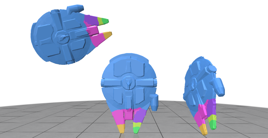
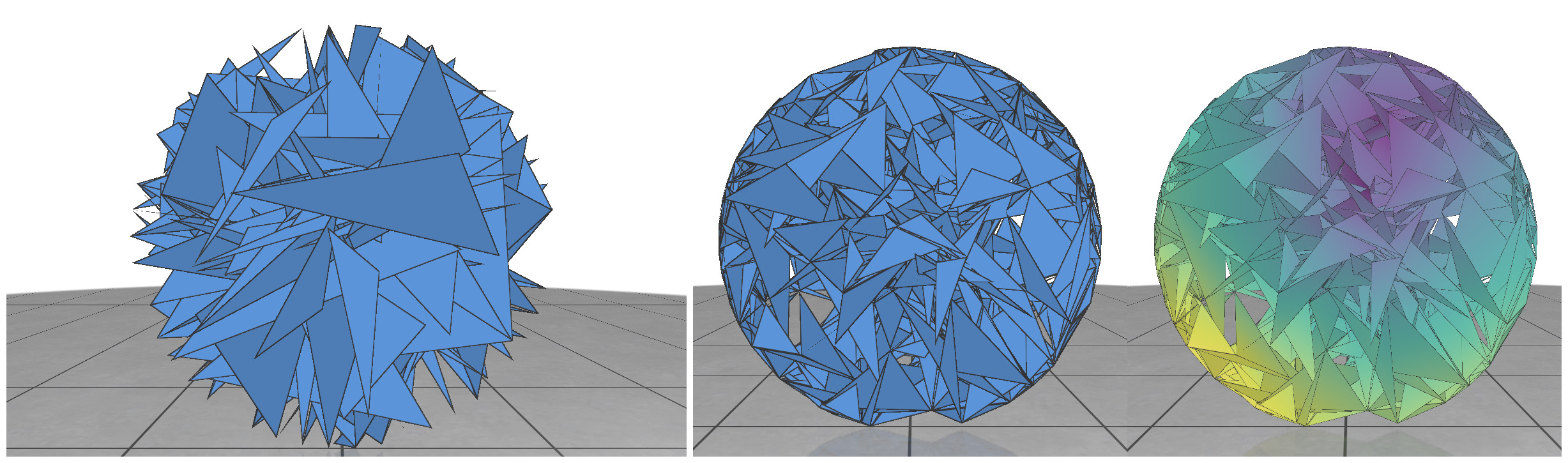
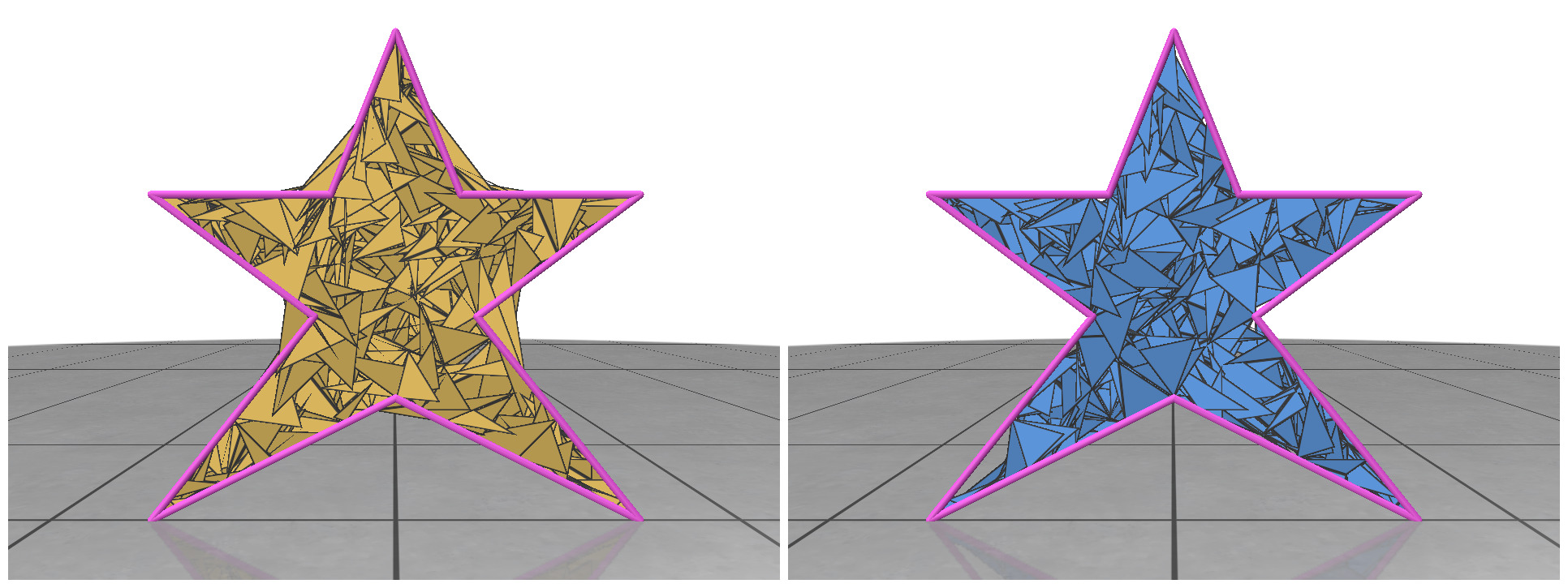
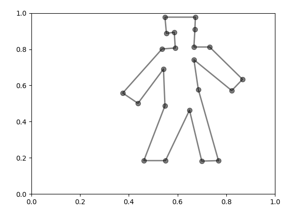
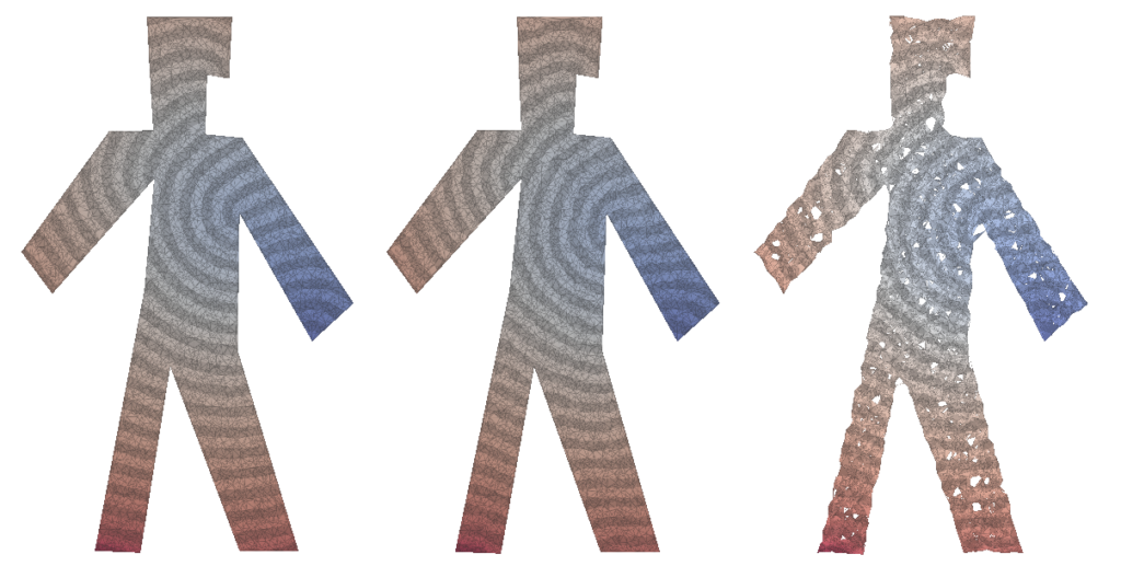
Fig 1: Even when all the pieces are rotated or translated with respect to the ground truth, it can still be a valid shape assembly.

While evaluating a predicted pose we must be careful, because the predicted values can be very different from the ground truth but can still describe a valid shape assembly. This is illustrated in Fig 1: We can rotate and translate all the pieces together by a certain amount that will result in a large value for our \(L^2\) metric, although this is a perfect shape assembly.

We solve this problem by measuring all the rotations and translations relative to one of the fragmented pieces.

Let’s assume we have two pieces:

Piece 1: rotation \(q_1\), translation \(t_1\)

Piece 2: rotation \(q_2\), translation \(t_2\)

Then the relative rotation and translation of Piece 2, with respect to Piece 1, can be calculated as:

\(q_{rel} = q_1^{-1} q_2\)

\(t_{rel} = q_1^{-1} (t_2-t_1) q_1\)

For both ground truth and prediction, we can calculate the relative rotations and translations of all the parts with respect to a chosen piece. Then we can easily use the \(L^2\) metrics defined above for comparison. This won’t affect the metric if all the pieces are moved together.

V. Codalab Challenge

We started implementing a Codalab challenge to explore this problem in all its complexities. For this, we set up a server that implemented the previously mentioned metrics and also started designing the type of submissions we could do.

Our scripts consisted in a code to evaluate the submissions in the Codalab server, the reference data we used to perform the evaluation and a starter-kit that could be used by people that are starting in the competition.

VI. References

[1] Silvia Sellán, Jack Luong, Leticia Mattos Da Silva, Aravind Ramakrishnan, Yuchuan Yang, Alec Jacobson. “Breaking Good: Fracture Modes for Realtime Destruction”. ACM Transactions on Graphics 2022.

[2] Silvia Sellán, Yun-Chun Chen, Ziyi Wu, Animesh Garg, Alec Jacobson. “Breaking Bad: A Dataset for Geometric Fracture and Reassembly”. Neural Information Processing Systems 2022.

Fellows: Aditya Abhyankar, Munshi Sanowar Raihan, Shanthika Naik, Bereket Faltamo, Daniel Perazzo

Volunteer: Despoina Paschalidou

Mentor: Nicholas Sharp

I. Introduction

Triangular and tetrahedral meshes are central to geometry, we use them to represent shapes, and as bases to compute with. Many numerical algorithms only actually work well on meshes that have nicely-shaped triangles/tetrahedra, so we try very hard to generate meshes which simultaneously:

Represent the desired shape
Have nicely-shaped elements and
Perfectly interlock to cover the domain with no gaps or overlaps.

Yet, is point (3) really that important? What if instead we just sampled a soup of random nicely-shaped triangles, and didn’t worry about whether they fit together?

In this project we explore several strategies for generating such random meshes, and evaluate their effectiveness.

II. Algorithms

II.1. Triangle Sampling

Fig 1: The heat geodesic method fails if the triangles are isolated (left); but if the triangles share vertex entries, the heat method works even with gaps and intersections (right).

In random meshing, we are given the boundary of a shape (e.g. the polygon outline of a 2D figure) and the task is to generate random meshes to tessellate the interior. Here, we will focus mainly on the planar case, where we generate triangles with 2D vertex positions. We will test the generated meshes by running the Heat Method [2], a simulation-based algorithm for computing distance within a shape. The very first shape we tried to tessellate is a circular disk.

Since a circle is a convex shape, we can choose three random points inside the circle and any triangle is guaranteed to stay within the shape. But generating isolated triangles like these is not a good strategy, because downstream algorithms like the heat method rely on shared vertices to communicate across the mesh. Without shared vertices, it is equivalent to running the algorithm individually on a bunch of separate triangles one at a time.

Next strategy: At each vertex, consider generating n random triangles that are connected to other vertices within a certain radius. This ensures that the generated triangles share the same vertex entries. Even though these random triangles have many gaps and intersections, many algorithms are actually perfectly well-defined on such a mesh. To our surprise, the heat method was able to generate reasonable results even with these random soup of triangles (Fig 1).

II.2. Non-Convex Shapes

Fig 2: Random meshing of a non-convex star shape (left); mesh generated by rejection sampling of the triangles (right).

For non-convex shapes, if we try to connect any three points within the polygon, some of the triangles might fall outside of our 2D boundary. This is illustrated in Fig 2 (left). To circumvent this problem, we can do rejection sampling of the triangles. Every time we generate a new triangle, we need to test whether it is completely contained within the boundary of our polygon. If it’s not, we reject it from our face list and sample another one. After rejection, the random meshes seem to nicely follow the boundary. Rejection sampling makes our meshing algorithm a little slower, but it’s necessary to handle non-convex shapes.

II.3. Triangle Size

Fig 3: Random meshes with different triangle size (left) and the isolines of their geodesic distance from the source (right).

In random meshes, we find that the performance of the heat geodesic method is dependent on the size of the triangles. Since we are generating triangles by sampling points within a radius, we can make the triangles smaller or larger by controlling the radius of the circle. With decreasing triangle size, the distance computed by the heat method becomes more accurate. This is illustrated in Fig 3: as the triangles become smaller, the isolines look more precise. The number of triangles are kept fixed in all cases.

III. Visualizations and results

We created an interface to aid in the task of drawing different polygon shapes for visualization. As can be seen below, an example of a shape:

We can use one of our algorithms to plot various types of meshes with the distance function drawn by the heat equation. We put the visualization of these meshes bellow, where the leftmost is the mesh using Delaunay triangulation, the rightmost using random triangles and the center being using Delaunay triangulation but using the faces from the Delaunay triangulation for a better visualization.

In this case, with 5000 points sampled randomly, we have an error of 0.0002 compared with the values for the distance function compared with using the heat method.

IV. An Attempt at Random Walk Meshing

Another interesting meshing idea is spawning a single vertex somewhere in the interior of the shape, and then iteratively “growing” the mesh from there in the style of a random walk. At each iteration, every leaf vertex randomly spawns two more child vertices on the circumference of a circle surrounding it, which are used to form a new face. If any such spawning circle intersects with the boundary of the shape, we simply use the two vertices of the closest boundary edge instead to form the new face. We tried various types of random walk strategies, such as using correlated random walks with various correlation settings to mitigate clustering at the source vertex.

While this produced an interesting single component random mesh, the sparse connectivity made it a bad algorithm for the heat method, as triangle sequences that swiveled back around in the direction of the source vertex diffused heat backwards in that direction too.

This caused the distance computations to be inaccurate and rendered the other methods superior. We would like to explore this approach further though, as it might prove useful for other use-cases like physics simulations and area approximations. Random walks are very well studied in probability literature too, so deriving theoretical results for such algorithms seems like a very principled task.

V. Structure in Randomness

While sampling triangles within a radius gave a reasonable results upon calculating geodesic distance, we tried exploring ways to make it more structured. One such method we came with is grid sampling with triangulation within a neighborhood. The steps are as follows:

Uniformly sample points within a square grid enclosing the entire shape.
Eliminate points outside that fall out of the desired shape.
For each vertex within the shape, form a fan of triangles with its 1 ring neighborhood vertices.

These are the geodesic isolines on the triangular mesh obtained using the above method.

VI. Conclusion and Future Work

We present some examples of our random computation method working on 2D meshes for various different shapes. Aside from refining our algorithms and performing more experiments, one interesting avenue would be to perform experiments with tetrahedralization on 3D shapes. We have also done simple tests with current state-of-the-art tetrahedralization algorithms [3], the results are shown below. So, for future work, this would be a really interesting avenue. Another interesting avenue for theoretical work regarding random walk meshing would be computing how the density of triangles varies with iteration count and various degrees of correlation.

VII. References

[1] Shewchuk, Jonathan Richard. “Triangle: Engineering a 2D quality mesh generator and Delaunay triangulator.” Workshop on applied computational geometry. Berlin, Heidelberg: Springer Berlin Heidelberg, 1996.

[2] Crane, Keenan, Clarisse Weischedel, and Max Wardetzky. “The heat method for distance computation.” Communications of the ACM 60.11 (2017): 90-99.

[3] Hu, Yixin, et al. “Tetrahedral meshing in the wild.” ACM Trans. Graph. 37.4 (2018): 60-1.

[4] Hu, Yixin, et al. “Fast tetrahedral meshing in the wild.” ACM Transactions on Graphics (TOG) 39.4 (2020): 117-1.