By SGI Fellows: Matheus da Silva Araujo and Shalom Bekele
Mentor: Mina Konaković Luković
Volunteers: Nicole Feng
I. Introduction
Kirigami is the Japanese art of creating 3D forms and sculptures by folding and cutting flat sheets of paper. However, its usages can be extended beyond artistic purposes, including material science, additive fabrication, and robotics [1, 2, 3]. In this project, mentored by Professor Mina Konaković Luković, we explored a specific regular cutting pattern called auxetic linkages, whose applications range from architecture [4] to medical devices [5], such as heart stents. For instance, thanks to the use of auxetic linkages, the Canopy Pavilion at EPFL (Lausanne, Switzerland) provides optimal shading while consuming less physical material. Specifically, we studied how to create these kirigami linkages computationally and how to satisfy their geometric and physical constraints as they deform. Video 1 demonstrates the results of deforming a kirigami linkage using the shape deformation techniques investigated in this project.
II. Auxetic Linkages
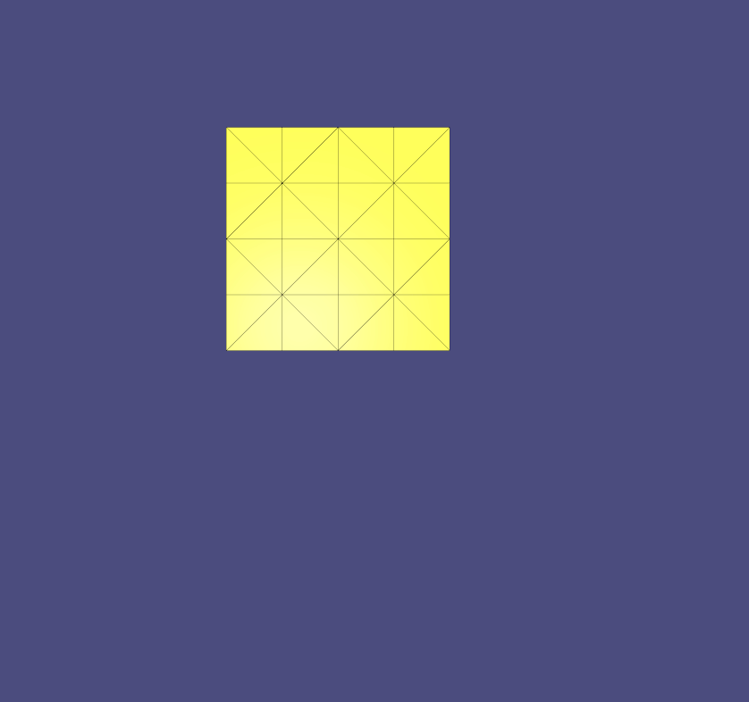
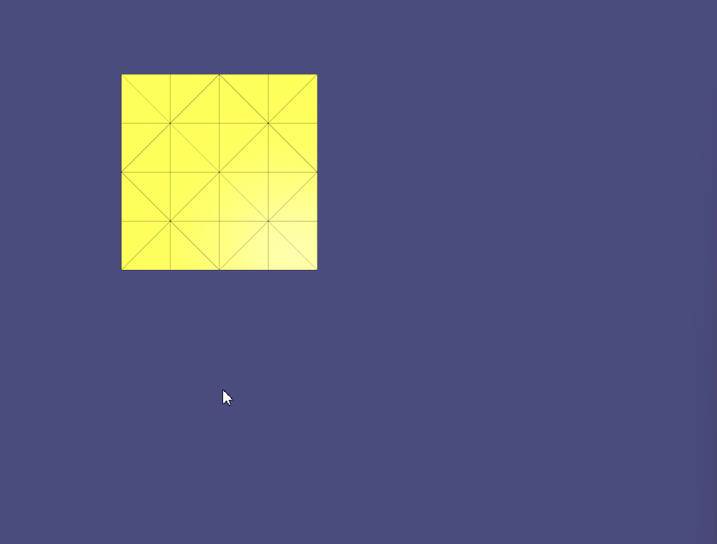
Auxetic linkages can be created through a specific cutting pattern that allows materials that would otherwise be inextensible to uniformly stretch up to a certain limit. This process provides further flexibility to represent a larger space of possible shapes because it makes it possible to represent shapes with non-zero Gaussian curvature. Figure 1 shows a real-life piece of cardboard cut using a rotating squares pattern.
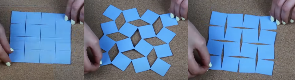
One possible way to generate a triangle mesh representing this particular pattern consists in creating a regular grid and implementing a mesh cutting algorithm. The mesh cutting is used to cut slits in the regular grid such that the final mesh represents the auxetic pattern. An alternative approach leverages the regularity of the auxetic pattern and generates the mesh by connecting an arrangement of rotating squares at its hinges [6].
III. As-Rigid-As-Possible Shape Deformation
To simulate and interact with kirigami linkages, we explored different algorithms to interactively deform these shapes while attempting to satisfy the geometric and physical constraints, such as rigidity and resistance to stretching.
The goal of shape deformation methods is to deform an initial shape while satisfying specific user-supplied constraints and preserving features of the original surface. Suppose a surface \(\mathcal{S}\) is represented by a triangle mesh \(\mathcal{M}\) with a set of vertices \(\mathcal{V}\). The user can constrain that some subset of vertices \(\mathcal{P} \in \mathcal{V}\) must be pinned or fixed in space while a different subset of vertices \(\mathcal{H} \in \mathcal{V}\) may be moved to arbitrary positions, e.g., moved using mouse drag as input. When vertices \(\mathcal{P}\) are fixed and vertices \(\mathcal{H}\) are moved, what should happen to the remaining vertices \(\mathcal{R} = \mathcal{V} \setminus (\mathcal{P} \cup \mathcal{H})\) of the mesh? The shape deformation algorithm must update the positions of the vertices \(\mathcal{R}\) in such a way that the deformation is intuitive for the user. For instance, the deformation should preserve fine details of the initial shape.
There are a lot of ways to try to define a more precise definition of what an “intuitive” deformation would be. A common approach is to define a physically-inspired energy that measures distortions introduced by the deformation, such as bending and stretching. This can be done using intrinsic properties of the surface. A thin shell energy based on the first and second fundamental forms is given by
\(\begin{equation}
E(\mathcal{S}, \mathcal{S}’) = \iint_{\Omega} k_{s} \| \mathbf{I}'(u, v) – \mathbf{I}(u, v) \|^{2} + k_{b} \| \mathbf{II}'(u, v) – \mathbf{II}(u, v) \|^{2} \text{d}u \text{d}v
\end{equation}\)
where \(\mathbf{I}, \mathbf{II}\) are the first and second fundamental forms of the original surface \(\mathcal{S}\), respectively, and \(\mathbf{I}’, \mathbf{II}’\) are the corresponding fundamental forms of the deformed surface \(\mathcal{S}’\), respectively. The parameters \(k_{s}\) and \(k_{b}\) are weights that represent the resistance to stretching and bending. A shape deformation algorithm aims to minimize this energy while satisfying the user-supplied constraints for vertices in \(\mathcal{H}, \mathcal{P}\). Animation 1 displays the result of a character being deformed. See Botsch et al. 2010 [7] for more details and alternative algorithms for shape deformation.

The classic as-rigid-as-possible [8] algorithm (also known as ARAP) is one example of a technique that minimizes the previous energy. The observation is that deformations that are locally as-rigid-as-possible tend to preserve fine details while trying to satisfy the user constraints. If the deformation from shape \(\mathcal{S}\) to \(\mathcal{S}’\) is rigid, it must be possible to find a rotation matrix \(\mathbf{R}_{i}\) that rigidly transforms (i.e., without scaling or shearing) one edge \(\mathbf{e}_{i, j} \) with endpoints \(\mathbf{v}_{i}, \mathbf{v}_{j}\) of \(\mathcal{S}\) into one edge \(\mathbf{e}_{i, j}’\) with endpoints \(\mathbf{v}_{i}’, \mathbf{v}_{j}’\) of \(\mathcal{S}’\):
\(\begin{equation}
\mathbf{v}_{i}’ – \mathbf{v}_{j}’ = \mathbf{R}_{i}(\mathbf{v}_{i} – \mathbf{v}_{j})
\end{equation}\)
The core idea of the method is that even when the deformation is not completely rigid, it is still possible to find the as-rigid-as-possible deformation (as implied in the name of the algorithm) by solving a minimization problem in the least-squares sense:
\(\begin{equation}
E(\mathcal{S}, \mathcal{S}’) = \sum_{i}^{n} w_{i} \sum_{j \in \mathcal{N}(i)} w_{ij} \| (\mathbf{v}_{i}’ – \mathbf{v}_{j}’) – (\mathbf{R}_{i} (\mathbf{v}_{i} – \mathbf{v}_{j})) \|^{2}
\end{equation}\)
The weights \(w_{i}\) and \(w_{ij}\) are used to make the algorithm more robust against discretization bias. In other words, depending on the mesh connectivity, the result may exhibit undesirable asymmetrical deformations. To mitigate these artifacts related to mesh dependence, Sorkine and Alexa [8] chose \(w_{i} = 1\) and \(w_{ij} = \frac{1}{2}(\cot \alpha_{ij} + \cot \beta_{ij})\), where \(\alpha_{ij}\) and \(\beta_{ij}\) are the angles that oppose an edge \(e_{ij}\). It is worth noting that the choice of \(w_{ij}\) corresponds to the cotangent-Laplacian operator, which is widely used in geometry processing.
Note that the positions of the vertices in \(\mathcal{H}\) and \(\mathcal{P}\) are known, since they are explicitly specified by the user. Hence, this equation has two unknowns: the positions of the vertices in \(\mathcal{R}\) and the rotation matrix \(\mathbf{R}_{i}\). ARAP solves this using an alternating optimization strategy:
- Define arbitrary initial values for \(\mathbf{v}_{i}’\) and \(\mathbf{R}_{i}\);
- Assume that the rotations are fixed and solve the minimization for \(\mathbf{v}_{i}’\);
- Using the solutions found in the previous step for \(\mathbf{v}_{i}’\), solve the minimization for \(\mathbf{R}_{i}\);
- Repeat steps (2) and (3) until some condition is met (e.g., a maximum number of iterations is reached).
By repeating this alternating process, the deformation energy is minimized and the as-rigid-as-possible solution can be computed. Video 2 shows our results using the ARAP implementation provided by libigl applied to a kirigami linkage. While one vertex on the top-row is constrained to be fixed in a position, the user can drag other vertices.
IV. Constraint-Based Shape Optimization
While ARAP is a powerful method, it is restricted to local feature preservation through rigid motions. Shape-Up [9] proposes a unified optimization strategy by defining shape constraints and projection operators tailored for specific tasks, including mesh quality improvement, parameterization and shape deformation. This general constraint-based optimization approach provides more flexibility: not only can it be applied to different geometry processing applications beyond shape deformation, but it also can be applied to point clouds, polygon meshes and volumetric meshes. Besides geometric constraints, this optimization method can be further generalized using projective dynamics [10] to incorporate physical constraints such as strain limiting, volume preservation or resistance to bending.
A set of \(m\) shape constraints \({ C_{1}, C_{2} , …, C_{m} }\) are used to describe desired properties of the surface. The shape projection operator \(P_{i}\) is responsible for projecting the vertices \(\mathbf{x}\) of the shape into the constraint set \(C_{i}\), i.e., finding the closest point to \(\mathbf{x}\), \(\mathbf{x}^{*}\), that satisfies the constraint \(C_{i}\). The nature of the constraints is determined by the application; for instance, physical and geometric constraints can be chosen based on fabrication requirements. A proximity function \(\mathbf{\phi}(\mathbf{x})\) is used to compute the weighted sum of squared distances to the set of constraints:
\(\begin{equation} \label{eq:optim-shapeup}
\mathbf{\phi} (\mathbf{x}) = \sum_{i = 1}^{m} w_{i} \| \mathbf{x} – P_{i}(\mathbf{x}) \|^{2} = \sum_{i = 1}^{m} w_{i} d_{i}(\mathbf{x})^{2}
\end{equation} \)
where \(d_{i}(\mathbf{x})\) measures the minimum distance between \(\mathbf{x}\) and the constraint set \(C_{i}\). The constraints may contradict each other in the sense that satisfying one constraint may cause the violation of the others. In this case, it may not be possible to find a point \(\mathbf{x}^{*}\) such that \(\mathbf{\phi} (\mathbf{x}^{*})= 0\); instead, a minimum in the least-squares sense can be found. \(w_{i}\) is a weighting factor that controls the influence of each constraint. Since it may not be possible to satisfy all the constraints simultaneously, by controlling \(w_{i}\) it is possible to specify more importance to satisfy some constraints by assigning it a larger weight in the equation.
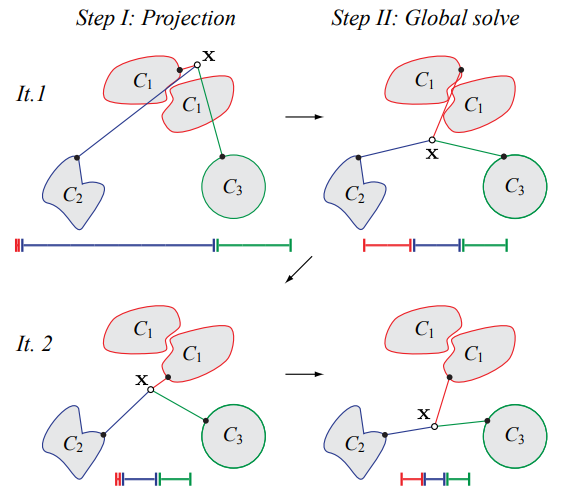
Figure 2 illustrates the algorithm. In each iteration, the first step (Figure 2, left) computes the projection of the vertex onto the constraint sets. That is, the closest points to \(\mathbf{x}\) in each constraint set are computed. Next, the second step (Figure 2, right) computes a new value for \(\mathbf{x}\) by minimizing \(\mathbf{\phi}(\mathbf{x})\) while keeping the projections fixed. In Figure 2, the colored bars denote the error of the current estimate \(\mathbf{x}\). Note that the sum of the bars (i.e., the total error) decreases monotonically, even if the error of a specific constraint increases (e.g., the error associated with the constraint \(C_{1}\) is larger by the end of the second iteration in comparison to the start). As previously mentioned, it may not be possible to satisfy all the constraints simultaneously, but the alternating minimization algorithm minimizes the overall error in the least-squares sense.
In practice, the optimization problem is solved for a set of vertices describing the shape, \(\mathbf{X}\), instead of a single position. The authors also incorporate a matrix \(\mathbf{N}\) to centralize the vertices \(\mathbf{X}\) around the mean, which can help in the convergence to the solution. The alternating minimization employed by ShapeUp is similar to the procedure described for ARAP:
- Define the vertices \(\mathbf{X}\), the constraints set \(\{ C_{1}, C_{2} , …, C_{m} \}\) and the shape projection operators \(P_{1}, P_{2}, …, P_{m}\);
- Assuming that the vertices \(\mathbf{X}\) are fixed, solve the minimization for \(P_{i}(\mathbf{N}_{i}\mathbf{X}_{i})\) using least-squares shape matching, where \(\mathbf{X}_{i} \subseteq \mathbf{X}\) denotes the vertices influenced by the constraint \(C_{i}\);
- Using the solutions found in the previous step for \(P_{i}(\mathbf{N}_{i}\mathbf{X}_{i})\), solve the minimization for \(\mathbf{X}\);
- Repeat steps (2) and (3) until some condition is met (e.g., a maximum number of iterations is reached).
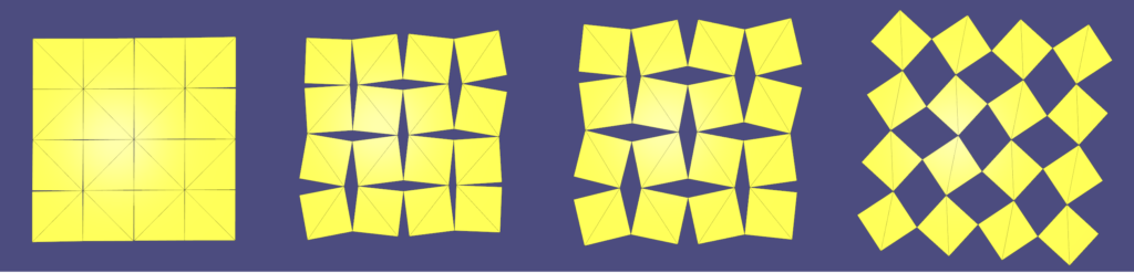
Figure 3 shows the result of the shape deformation for a kirigami linkage, where the bottom-left corner was constrained to stay in the initial position while the top-right corner was constrained to move to a different position. The remaining vertices are constrained to move while preserving the edge lengths i.e., without introducing stretching during shape deformation. The results shown represent the solution found by the optimization method for 8, 16, 64 and 256 iterations (left to right). Depending on the particular position that the top-right corner was constrained to move to, it may not be possible to find a perfectly rigid transformation. However, as was the case with ARAP, the alternating minimization process will find the best solution in the least squares sense. The advantage of ShapeUp is the possibility to introduce different and generic types of constraints.
ShapeUp and Projective Dynamics were combined in the ShapeOp [11] framework to support both geometry processing and physical simulation in a unified solver. The framework defines a set of energy terms that quantify each constraint’s deviation. These energy terms are usually quadratic or higher-order functions that quantify the deviation from the desired shape. ShapeOp finds an optimal shape configuration that satisfies the constraints by minimizing the overall energy of the system. For dynamics simulation tasks, ShapeOp employs the Projective Implicit Euler integration scheme, where the physical and geometric constraints are resolved using the local-global solver described below at each integration step. ShapeOp provides stability, typical of implicit methods, while providing a lower computational cost due to the efficiency of the local-global alternating minimization.
In this framework, physical energy potentials and geometric constraints are solved in a unified manner. Each solver iteration consists of a local step and a global step defined as follows:
- Local Step: for each set of points that is commonly influenced by a constraint, a candidate shape is computed. For a geometric constraint, this entails fitting a shape that satisfies the constraint, e.g., constraining a quadrilateral to be deformed into a square. For a physical constraint, this was reduced to locating the nearest point positions with zero physical potential value.
- Global Step: the candidate shapes computed in the local step may be incompatible with each other. For instance, this may happen if the satisfaction of one constraint causes the violation of another constraint. The global step finds a new set of consistent positions so that each set of points subject to a common constraint is as close to the corresponding candidate shape as possible.
Animations 2 and 3 present the results of simulating a kirigami linkage under the effect of gravity (i.e., the force gravity is applied as an external force to the system) using ShapeOp framework and libigl. The edge strain constraint is used to simulate strain limiting. The closeness constraint is used to fix the position of two vertices on the top-row; this constraint projects the vertices into a specific rest position.
For Animation 2, the weights of the edge strain and closeness constraints were \(w_{i} = 1000\) and \(w_{i} = 100\), respectively. As can be seen in Animation 2, the kirigami presents noticeable stretching, which is undesirable for near-rigid linkages. This means that this weighting scheme doesn’t provide sufficient importance to the edge strain constraint to guarantee strain limiting. Nonetheless, this shows that the shape optimization approach of ShapeUp and Projective Dynamics provide flexibility to design and simulate a wide range of constraints and materials depending on the goal.
Animation 3 shows a simulation similar to Animation 2, but the weights of edge strain constraint and closeness constraint were \(w_{i} = 5000\) and \(w_{i} = 100\), respectively. In this case, the deformation is closer to a rigid motion and presents significantly less stretching.
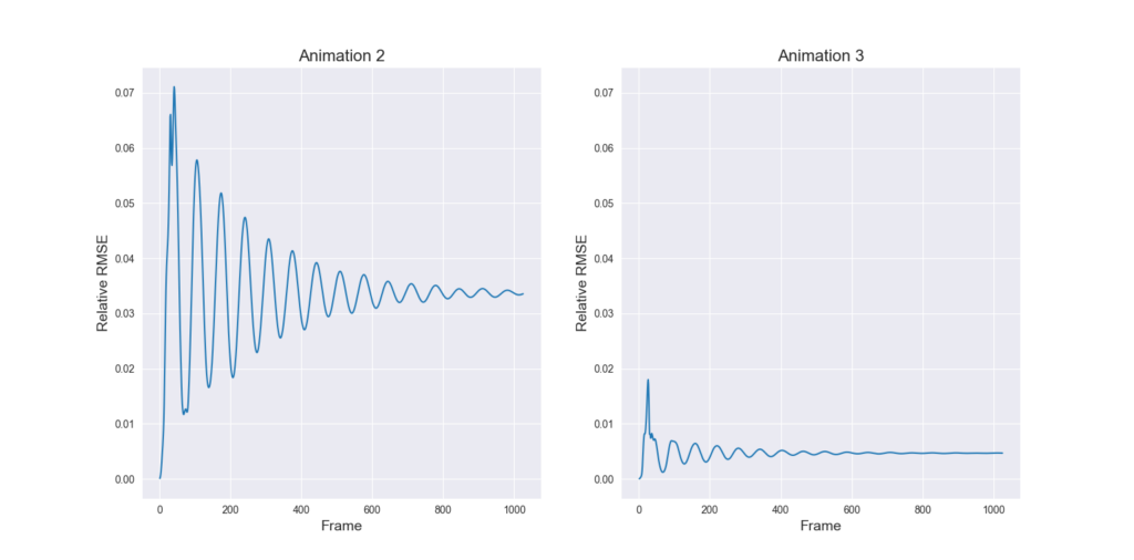
Figure 4 presents a quantitative comparison between Animation 2 (Figure 4, left) and Animation 3 (Figure 4, right) using the relative root-mean-squared error to measure the edge length distortion introduced during the simulation. As can be seen, Animation 3 exhibits considerably less stretching and converges to a final solution in fewer frames. As mentioned, this is caused by the fact that Animation 3 uses a larger weight to satisfy the edge strain constraint. By giving priority to satisfying the edge strain constraint, the edge length distortion is reduced. However, note that the final result for both Animation 2 and Animation 3 have an error greater than zero, indicating that the constraint set imposed cannot be perfectly satisfied.
Finally, Animation 4 displays a simulation that also incorporates a user-supplied external force. In this simulation, besides the gravitational force, one vertex is also subject to a per-vertex force that drags it to the right. For instance, this force may be controlled by the user through mouse input. As the simulation executes, the kirigami is subject to both external forces and to the constraint sets. As before, the edge strain and closeness constraints were added to the optimization process.
V. Conclusions and Future Work
In this project we explored various geometric and physical aspects of kirigami linkages. By leveraging various techniques from geometry processing and numerical optimization, we could understand how to design, deform and simulate near-rigid materials that present a particular cutting pattern – the auxetic linkage.
As future work we may explore new types of constraints such as non-interpenetration constraints to prevent one triangle from intersecting others. Moreover, by using conformal geometry, we may replicate the surface rationalization approach of Konaković et al. 2016 [12] to approximate an arbitrary 3D surface using the auxetic linkage described above.
We would like to thank Professor Mina Konaković for the mentoring and insightful discussions. We were impressed by the vast number of surprising applications that could arise from an artistic pattern, ranging from fabrication and architecture to robotics. Furthermore, we would like to thank the SGI volunteer Nicole Feng for all the help during the project week, particularly with the codebase. Finally, this project would not have been possible without Professor Justin Solomon, so we are grateful for his hard work organizing SGI and making this incredible experience possible.
VI. References
[1]: Rubio, Alfonso P., et al.”Kirigami Corrugations: Strong, Modular and Programmable Plate Lattices.” ASME 2023 International Design Engineering Technical Conferences and Computers and Information in Engineering Conference (IDETC-CIE2023),(2023).
[2]: Dudte, Levi H., et al. “An additive framework for kirigami design.” Nature Computational Science 3.5 (2023): 443-454.
[3]: Yang, Yi, Katherine Vella, and Douglas P. Holmes. “Grasping with kirigami shells.” Science Robotics 6.54 (2021): eabd6426.
[4]: Konaković-Luković, Mina, Pavle Konaković, and Mark Pauly. “Computational design of deployable auxetic shells.” Advances in Architectural Geometry 2018.
[5]: Konaković-Luković, Mina, et al. “Rapid deployment of curved surfaces via programmable auxetics.” ACM Transactions on Graphics (TOG) 37.4 (2018): 1-13.
[6]: Grima, Joseph N., and Kenneth E. Evans. “Auxetic behavior from rotating squares.” Journal of materials science letters 19 (2000): 1563-1565.
[7]: Botsch, Mario, et al. Polygon mesh processing. CRC press, 2010.
[8]: Sorkine, Olga, and Marc Alexa. “As-rigid-as-possible surface modeling.” Symposium on Geometry processing. Vol. 4. 2007.
[9]: Bouaziz, Sofien, et al. “Shape‐up: Shaping discrete geometry with projections.” Computer Graphics Forum. Vol. 31. No. 5. Oxford, UK: Blackwell Publishing Ltd, 2012.
[10]: Bouaziz, Sofien, et al. “Projective Dynamics: Fusing Constraint Projections for Fast Simulation.” ACM Transactions on Graphics 33.4 (2014): Article-No.
[11]: Deuss, Mario, et al. “ShapeOp—a robust and extensible geometric modelling paradigm.” Modelling Behaviour: Design Modelling Symposium 2015. Springer International Publishing, 2015.
[12]: Konaković, Mina, et al. “Beyond developable: computational design and fabrication with auxetic materials.” ACM Transactions on Graphics (TOG) 35.4 (2016): 1-11.